Developing an ice strength algorithm for sub-Arctic regions

(1)

Publisher’s version / Version de l'éditeur: Technical Report, 2004-03

READ THESE TERMS AND CONDITIONS CAREFULLY BEFORE USING THIS WEBSITE. https://nrc-publications.canada.ca/eng/copyright

Vous avez des questions? Nous pouvons vous aider. Pour communiquer directement avec un auteur, consultez la

première page de la revue dans laquelle son article a été publié afin de trouver ses coordonnées. Si vous n’arrivez pas à les repérer, communiquez avec nous à [email protected].

Questions? Contact the NRC Publications Archive team at

[email protected]. If you wish to email the authors directly, please see the first page of the publication for their contact information.

For the publisher’s version, please access the DOI link below./ Pour consulter la version de l’éditeur, utilisez le lien DOI ci-dessous.

https://doi.org/10.4224/12329076

Access and use of this website and the material on it are subject to the Terms and Conditions set forth at

Developing an ice strength algorithm for sub-Arctic regions

Johnston, M.; Timco, G.

https://publications-cnrc.canada.ca/fra/droits

L’accès à ce site Web et l’utilisation de son contenu sont assujettis aux conditions présentées dans le site LISEZ CES CONDITIONS ATTENTIVEMENT AVANT D’UTILISER CE SITE WEB.

NRC Publications Record / Notice d'Archives des publications de CNRC:

https://nrc-publications.canada.ca/eng/view/object/?id=a8b34fc6-0708-4f0f-a349-f7e6b0180d2f https://publications-cnrc.canada.ca/fra/voir/objet/?id=a8b34fc6-0708-4f0f-a349-f7e6b0180d2f

(2)

Developing an Ice Strength Algorithm

for Sub-Arctic Regions

M. Johnston and G. Timco

Resolute 0.69 MPa Chesterfield 0.67 MPa Churchill 0.63 MPa Moosonee 0.51 MPa Nain 0.53 MPa 8 Feb Resolute 0.65 MPa Chesterfield 0.57 MPa Churchill 0.46 MPa Moosonee NA Nain 0.26 MPa 18 Apr

Technical Report, CHC-TR-023

March 2004

(3)

(4)

Developing an Ice Strength Algorithm

for Sub-Arctic Regions

M. Johnston and G. Timco Canadian Hydraulics Centre National Research Council of Canada

Montreal Road Ottawa, Ontario K1A 0R6

Prepared for: Canadian Ice Service 373 Sussex Drive, Bld. E-3 Ottawa, Ontario K1A 0H3

Technical Report, CHC-TR-023 March 2004

(5)

(6)

Abstract

This study, the first year of a two-year study, was undertaken to determine whether the algorithm that is used to describe the seasonal decrease in strength of landfast, first-year ice in the high Arctic can also be used for sub-Arctic first-year ice. The strength algorithm is the basis of the Ice Strength Charts issued by Canadian Ice Service. The method used to formulate an Ice Strength Algorithm for the high Arctic and its applicability for sub-Arctic ice are discussed. The report outlines the steps taken to develop the strength algorithm for sub-Arctic areas. Relevant data on the properties of sub-Arctic ice are compiled and an approach for including sub-Arctic regions in future Ice Strength Charts is suggested. Emphasis is given to level first-year ice along the Labrador coast and in Hudson Bay.

(7)

(8)

List of Figures

Figure 1 Flexural strength versus the square root of the brine volume for first-year sea ice ...3

Figure 2 Comparison of two techniques for calculating flexural strength ...4

Figure 3 Sites for which air temperature and ice thickness data were supplied ...5

Figure 4 Two-week, smoothed 30-yr MDT for sites...6

Figure 5 Ice thickness data for Moosonee and Resolute...8

Figure 6 Comparison of ice thickness obtained from polynomial expression...9

Figure 7 Seasonal decrease in flexural strength and ice thickness at different sites ...10

Figure 8 Calculated flexural strength, expressed in terms of Julian Day ...13

Figure 9 Calculated flexural strength, expressed in terms of air temperature ...14

Figure 10 Ice borehole strength and flexural strength versus bulk ice temperature ...15

Figure 11 Flexural strength, normalized by mid-winter strength of Arctic ice ...16

Figure 12 Flexural strength, normalized by maximum strength at each site...17

Figure 13 Flexural strength in terms of physical units ...17

Figure 14 Accumulated degree-days from baseline of -35°C and start date of January 1 ...18

Figure 15 Seasonal decrease in ice strength as function of accumulated degree days...19

Figure 16 2002 MDT, 7-day ave of 2002 MDT and the 2-week smoothed 30-yr MDT ...21

Figure 17 Calculated flexural strength for Resolute using 2002 MDT ...21

Figure 18 Calculated flexural strength of first-year ice from February to June ...23

List of Tables

Table 1 Climate at Each of the Selected Sites, based on smoothed 30-yr MDT ...7

Table 2 Duration of Historical Data on Ice Thickness Measurements...7

Table 3 Calculated Flexural Strengths for Selected Sites...11

(11)

(12)

Developing an Ice Strength Algorithm

for Sub-Arctic Regions

1.0 Introduction

From 2000 to 2002, the Canadian Hydraulics Centre (CHC) conducted measurements on first-year ice in the high Arctic to document changes occurring in the ice from spring to summer. Field measurements included snow and ice thickness, ice temperature and salinity and the in situ ice borehole strength. Data acquired during those three years were used to formulate an equation, or strength algorithm, that was used as the basis for prototype Ice Strength Charts. The Ice Strength Charts have been issued by Canadian Ice Service (CIS) from May to August. To date, they have been issued only for landfast, level first-year ice in the high Arctic. This study was undertaken to assess the possibility of using the same algorithm, or developing a new one, to describe the strength of ice south of the Arctic, in the so-called sub-Arctic.

The cursory examination conducted by Johnston and Timco (2003-a) showed that the strength algorithm for first-year ice in the high Arctic should not be extended to the same ice type in sub-Arctic areas. Developing an algorithm for ice south of 60°N would require the following:

• itemize steps needed to develop a strength algorithm for sub-Arctic areas

• literature search to compile previously-measured properties of sub-Arctic ice

• develop an approach for including sub-Arctic regions in future Ice Strength Charts

This report, the first of a two-year study, provides an overview of the work done on the above-mentioned tasks. The mandate given to CHC by CIS indicated that emphasis should be given to level first-year ice along the Labrador coast and in Hudson Bay. During the second year of this project the proposed approach for including sub-Arctic ice in future Ice Strength Charts will be examined using temperature, salinity and strength measurements recently acquired on landfast, level first-year ice near Nain, Labrador. The Labrador field study is a two-year project that was sponsored jointly by Transport Canada and Canadian Ice Service. It will provide much needed data on the properties of sub-Arctic ice and their changes throughout spring and summer.

(13)

2.0 Outline of the Report

A number of steps were taken to develop an approach for including sub-Arctic ice in future Ice Strength Charts. This report documents those steps, which included:

• obtaining data to calculate the flexural strength of first-year ice

• examining air temperatures and ice thicknesses at five sites on Labrador Coast and in Hudson Bay

• calculating the seasonal decrease in flexural strength at those selected sites using mean daily air temperatures and estimated ice thickness

• calculating the flexural strength using existing ice property measurements and comparing them to calculations based on air temperatures and ice thickness

• examining the feasibility of relating the flexural strength of ice to accumulated degree days (ADD) at different latitudes

• basing future Ice Strength Charts on flexural strengths calculated directly from established equations

• using strength maps to visualize the decrease in strength of Arctic and sub-Arctic ice

• conclusions and recommendations

• literature review – list of abstracts

3.0 Approaches for Calculating the Flexural Strength of Ice

Several researchers have attempted to relate the strength of sea ice to the brine volume or total porosity of the ice. There is a good reason for this. It is generally assumed that as the total porosity in the ice increases, the strength should decrease. That is because there is less "solid ice" that has to be broken. Timco and O’Brien (1994) conducted the most comprehensive analysis of the flexural strength of ice. Their analysis was based upon approximately 1000 tests on sea ice and used over 2500 reported measurements on the flexural strength of freshwater ice and sea ice. The authors showed that the data for first-year sea ice could be described by the following equation: ) * 88 . 5 ( exp 76 . 1 _b f υ σ = − (1)

where σ f is the flexural strength of the ice and the brine volume (νb) is expressed as a brine

(14)

0 0.5 1 1.5 2 0 0.1 0.2 0.3 0.4 0.5 0.6

Square Root of Brine Volume (νb) 1/2

Flexural Strength (MPa)

First-year Sea Ice

Average value for freshwater ice

σf = 1.76 exp [-5.88*sqrt(νb)]

Figure 1 Flexural strength versus the square root of the brine volume for first-year sea ice

There are several points to note from Figure 1:

• The value of 1.76 MPa for zero brine volume is in excellent agreement with the average strength (1.73 MPa) measured for freshwater ice.

• The general scatter in the data increases with decreasing brine volume. This is a reflection of the fact that, at low brine volumes, the ice shows brittle behavior. The range of scatter approaches that measured for freshwater ice and is characteristic of a brittle material.

• This equation is the most comprehensive equation for flexural strength to date. There have been a few other equations proposed to relate strength and brine volume however those were based on substantially fewer data points and data that extended over a very limited range. In other words, the other equations are valid over only a small brine volume range. The wider range of this equation represents these other equations very well in the ranges in which they are valid.

• Data for the equation were compiled from a large number of investigators and from a variety of geographic locations in both polar and temperate climates. Therefore it should be quite representative of the flexural strength of sea ice in most regions.

• The brine volume used to represent the ice beam for any test was taken as the average brine volume, determined from the average ice temperature and salinity of the beam. Calculations of the flexural strength require the depth-averaged temperature of the ice (or bulk temperature) and depth-averaged salinity of the ice (bulk ice salinity).

(15)

3.1 Intrinsic versus Extrinsic Method of Calculating Flexural Strengths

The so-called intrinsic method can be used to calculate the flexural strength of the ice using measured, depth profiles of the ice temperature and ice salinity (which are intrinsic ice properties). If those ice property measurements are not available, an extrinsic method can be used to calculate the flexural strength of the ice. The extrinsic method uses the air temperature and ice thickness to estimate the depth-averaged (bulk) ice temperature and bulk ice salinity (Timco and Frederking, 1990).

Figure 2 shows the comparison between the flexural strengths calculated using the two different techniques. In case (a) the flexural strength was calculated by the intrinsic method, using the ice temperature and ice salinity (T_ice and S_ice) measured on first-year ice in the high Arctic in 2000 and 2001. In case (b), the flexural strength was calculated from the air temperature and ice thickness (T_air and h_ice) recorded in the high Arctic during the same period. The figure shows that the extrinsic method usually results in lower strengths than the intrinsic method, although the strengths on Julian Day (JD) 142 and JD149 were higher. It should be noted that the intrinsic method is preferred for calculating the flexural strength of the ice, however measuring ice properties can be both difficult and costly.

0 0.1 0.2 0.3 0.4 0.5 0.6 130 135 140 145 150 155 160 Julian Day (JD)

Calculated flexural strength (MPa)

T_ice, S_ice T_air, h_ice

Figure 2 Comparison of two techniques for calculating flexural strength intrinsic method (T_ice and S_ice) vs. extrinsic method (T_air and h_ice)

(16)

4.0 Air temperature and Ice Thickness at Selected Sites

Since few property measurements have been made on ice along the Labrador Coast and virtually no measurements have been made on the ice in Hudson Bay (see literature review in Appendix A), it was necessary to use the extrinsic method for calculating the flexural strength of ice at different latitudes. As a result, Canadian Ice Service supplied CHC with air temperature and ice thickness data for nine climate stations in the area of interest, as shown in Figure 3.

Moosonee Churchill

Inukjuak Kuujjuak Nain Chesterfield

Resolute

Dorset Iqualuit

Figure 3 Sites for which air temperature and ice thickness data were supplied

Although air temperature and ice thickness data were provided for nine sites, CIS suggested that efforts be focused upon ice along the Labrador coast and the western regions of Hudson Bay, since that is where shipping is most extensive. Therefore, only five of the sites in Figure 3 were included in this analysis: Nain, Moosonee, Churchill, Chesterfield and Resolute, each of which is labeled on a darkened background in Figure 3. Resolute was included in this analysis, for comparative purposes only, because its three years of property measurements had been used to derive an ice strength algorithm for the high Arctic (Johnston and Timco, 2003-a).

4.1 Air Temperatures at Selected Sites

Air temperatures were supplied for each of the sites shown in Figure 3. The supplied data represented two-week averages of the 30-year normal mean daily air temperatures (designated as the ‘smoothed’ 30-yr MDT). For purposes of continuity between the two consecutive years, the figure shows Julian Days (JD) extending beyond JD365.

(17)

-50 -40 -30 -20 -10 0 10 20 0 200 400 600 800 Julian Day Smoothed 30-yr MDT (°C) Resolute Chesterfield Churchill Moosonee Nain

Figure 4 Two-week, smoothed 30-yr MDT for sites

Table 1 lists the minimum and maximum smoothed 30-yr MDT for each site and the dates on which they occur, along with the length of summer at the different sites. Summer was defined by the number of days that the smoothed 30-yr MDT remained above 0°C. Moosonee, the most southerly site, has the longest summer (196 days) and Resolute the shortest (72 days). Minimum temperatures at Nain and Moosonee are similar in winter (-20°C), however Moosonee experiences its coldest temperature about one week before Nain. In summer, temperatures in Nain are more like Churchill, with a maximum temperature of about +12°C that occurs on 30 July (JD576). In comparison, the maximum, smoothed 30-yr MDT at Moosonee is +16.5°C in summer and occurs on 26 July (JD572). Minimum averaged MDT at Resolute and Chesterfield are similar (-32°C and -33°C) although the coldest temperature in Resolute occurs about one month later than Chesterfield. As a result, the two sites have different lengths of winter. The summer maximum 30-yr MDT at Resolute and Chesterfield occur about the same time (16 July, JD562), yet differ by several degrees (+4.6°C in Resolute and +10.9°C in Chesterfield).

(18)

Table 1 Climate at Each of the Selected Sites, based on smoothed 30-yr MDT

Site Min temp (°C)/ Date Max temp (°C)/ Date Summer

(days)

Summer season Moosonee -20.3°C/ 13 Jan (JD378) +16.5°C / 26 Jul (JD572) 196 23 Apr-5 Nov (JD113-309)

Nain -20.2°C / 28 Jan (JD393) +11.9°C / 30 Jul (JD576) 170 7 May -24 Oct

(JD127-297) Churchill -26.9°C / 18 Jan (JD383) +12.7°C / 31 Jul (JD567) 142 20 May-9 Oct

(JD140-282) Chesterfield -32.0°C / 18 Jan (JD383) +10.9°C / 21 Jul (JD567) 120 1 Jun-29 Sep (JD152-272)

Resolute -33.4°C / 24 Feb

(JD420)

+4.6°C / 16 Jul (JD562) 72 16 Jun-27 Aug

(JD167-239)

4.2 Ice Thickness at Selected Sites

Canadian Ice Service provided CHC with digital information on the mean ice thickness for the five selected sites shown in Figure 3. The ice thickness data were compared to the ice thicknesses measured each year at the selected sites (Bilello, 1960, 1980; Bilello and Bates, 1991) and those from the CIS website (http://ice-glaces.ec.gc.ca).

Table 2 lists the years over which data were collected at each of the sites and the total number of data points for each site. In general, ice thickness measurements were made several times each week at the different sites. Since ice thickness information was not available for Nain, data were included for Hopedale, a coastal community 150 km south of Nain.

Table 2 Duration of Historical Data on Ice Thickness Measurements

Site Measurement years Data points

Moosonee 1959 - 1993 628

Hopedale 1960 - 1984 336

Churchill 1960 - 1987 465

Chesterfield 1959 - 1981 612

(19)

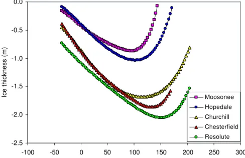
Figure 5 shows ice thickness data for the southern most (Moosonee) and northernmost (Resolute) sites. The figure shows historical ice thicknesses (circular data markers), a polynomial fit through the historical thickness data (solid line) and mean ice thickness data provided by CIS (yellow triangular data markers). Comparison shows that although there is a wide range of scatter in ice thickness measurements over the years, the CIS data agree favorably with the polynomial curve (solid line). The polynomials for calculating the seasonal increase and decrease in ice thickness for the five sites are included in Appendix B, expressed as a function of the continuous, two-year Julian Day. Appendix B also contains plots of measured and calculated ice thicknesses for all five sites.

Figure 6 compares results from the five polynomials that describe the increase and decrease in ice thickness at each site. The ice thickness at Hopedale and Moosonee are comparable. That is not surprising, considering air temperatures at the two sites were also similar during winter. What is surprising, however, is that the mean ice thicknesses at Churchill, Chesterfield and Resolute are all in good agreement. Recall that the mid-winter minimum 30-yr MDT for Churchill was about 10°C warmer than either Chesterfield or Resolute (about -32°C, Figure 4). Bilello (1980) states that the Churchill ice thickness measurements were frequently made near the mouth of the Churchill River, where the ice would have been thicker than typical first-year sea ice in that region. Other measurements were made in Churchill Harbour (Bilello and Bates, 1991; Bilello and Lunardini, 1996). The anomaly should be kept in mind when comparing the ice at Churchill to the other sites.

-2.5 -2.0 -1.5 -1.0 -0.5 0.0 250 300 350 400 450 500 550 600 650 700 Julian Day

Ice thickness (m) Moosonee

Moose h_i mean (m) Poly. (Moosonee) -2.5 -2.0 -1.5 -1.0 -0.5 0.0 250 300 350 400 450 500 550 600 650 700 Julian Day

Ice thickness (m) Resolute

Resolute, h_i mean (m) Poly. (Resolute)

(a) Moosonee (b) Resolute

Figure 5 Ice thickness data for Moosonee and Resolute (see Appendix B for additional sites)

(20)

-2.5 -2.0 -1.5 -1.0 -0.5 0.0 -100 -50 0 50 100 150 200 250 300

Julian Day (shifted to produce continuity between years)

Ice thickness (m) _Moosonee

Hopedale Churchill Chesterfield Resolute

Figure 6 Comparison of ice thickness obtained from polynomial expression

5.0 Flexural Strength of sub-Arctic Ice using MDT and Ice Thickness

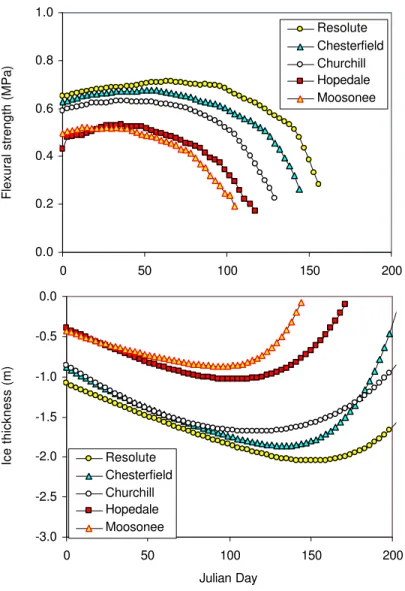
Figure 7 shows the flexural strengths calculated using the smoothed 30-yr MDT and mean ice thickness data1 for each site. The figure makes four points immediately apparent: 1) as expected, the maximum flexural strength differs for each site, 2) the initial decrease in ice strength at each site occurs at different times, 3) the decrease in strength follows a similar trend for each site and 4) the strength begins to decrease well before the ice begins to ablate.

5.1 Peak Flexural Strength of Ice at Different Latitudes

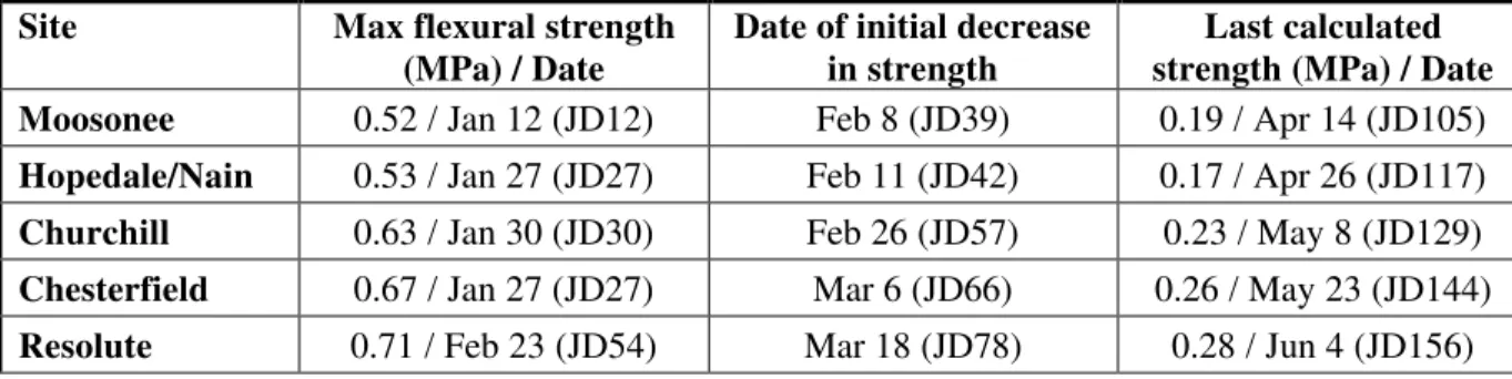
Table 3 lists the peak, calculated flexural strengths for each site and shows the date on which they occur. Peak flexural strengths for the five selected sites ranged from 0.52 to 0.71 MPa and showed a systematic decrease with decreasing latitude (Figure 7). The sites fall into two groups, each with similar ice thicknesses and flexural strengths. The first group consists of Moosonee and Nain and the second group includes Churchill, Chesterfield and Resolute. The anomalously thick ice at Churchill resulted in flexural strengths that were 0.10 MPa greater than the ice strength determined for Nain or Moosonee. Flexural strengths for the Churchill site should be reassessed should more accurate ice thickness measurements come available.

1

(21)

0.0 0.2 0.4 0.6 0.8 1.0 0 50 100 150 200 Julian Day

Flexural strength (MPa)

Resolute Chesterfield Churchill Hopedale Moosonee -3.0 -2.5 -2.0 -1.5 -1.0 -0.5 0.0 0 50 100 150 200 Julian Day Ice thickness (m) Resolute

Chesterfield Churchill Hopedale Moosonee

Figure 7 Seasonal decrease in flexural strength and ice thickness at different sites

Figure 7 shows that level first-year ice at Moosonee had the lowest calculated flexural strength. The maximum for that site was 0.52 MPa and occurred on January 12 (JD12). In comparison, the peak, calculated flexural strength at Resolute was 0.71 MPa and occurred on February 23 (JD54). The ice strengths at the different sites and their seasonal trends are significant because they show that the warmer temperatures in sub-Arctic areas result in a shorter ice growth season, which prevents the ice from developing a strength comparable to Arctic ice. For the most part, sub-Arctic ice has a peak flexural strength that occurs earlier and begins to decrease sooner than ice in the Arctic, as discussed subsequently.

(22)

Table 3 Calculated Flexural Strengths for Selected Sites

Site Max flexural strength

(MPa) / Date

Date of initial decrease in strength

Last calculated strength (MPa) / Date

Moosonee 0.52 / Jan 12 (JD12) Feb 8 (JD39) 0.19 / Apr 14 (JD105)

Hopedale/Nain 0.53 / Jan 27 (JD27) Feb 11 (JD42) 0.17 / Apr 26 (JD117)

Churchill 0.63 / Jan 30 (JD30) Feb 26 (JD57) 0.23 / May 8 (JD129)

Chesterfield 0.67 / Jan 27 (JD27) Mar 6 (JD66) 0.26 / May 23 (JD144)

Resolute 0.71 / Feb 23 (JD54) Mar 18 (JD78) 0.28 / Jun 4 (JD156)

5.2 Initial Seasonal Decrease in Flexural Strength

Because the sub-Arctic has a shorter ice growth season, its first-year ice is thinner and begins to decrease in strength earlier than first-year ice in the Arctic. Based upon the calculations, the strength of first-year ice near Moosonee begins to decrease around February 8 (JD39). Ice near Nain begins to lose strength three days later, on February 11 (JD42). At Churchill, Chesterfield and Resolute, the ice strength begins to decrease on February 26, March 6 and March 18 respectively.

The data compiled by Timco and O’Brien (1994) do not support using the relation between flexural strength and brine volume beyond a square root of brine volume fraction of 0.5. Above that value, excessive brine volume causes inaccuracies in the flexural strengths measured from prepared samples -- measurements upon which the equation is based. Table 3 lists the dates to which the calculated flexural strengths are valid and the strength corresponding to that date. Based upon the smoothed 30-yr MDT and mean ice thickness, the technique developed by Timco and O’Brien (1994) can be used to calculate the flexural strength of ice near Moosonee and Nain until mid to late-April, by which time the strength is near 0.18 MPa (compared to a maximum of 0.52 MPa). The flexural strength at Churchill can be calculated until about the first week of May whereas it can be calculated until late May and early June at Chesterfield and Resolute, respectively. Had ice property measurements been available for those sites, the flexural strengths could have been calculated about one month later (Johnston and Timco, 2003-a).

5.3 Relation between Decrease in Ice Strength and Ice Ablation

Realizing the limitations of the flexural strength equation, the borehole jack system was used to measure the seasonal decrease of strength in Arctic first-year ice from 2000 to 2002. The borehole jack is extremely valuable because it provides a measure of the in situ ice strength, which does not require sample preparation. In regions where data overlap, the borehole strength of Arctic ice showed the same type of seasonal decrease in strength observed in the calculated flexural strengths (Johnston et al., 2002).

(23)

The borehole jack tests showed that the decrease in ice strength precedes the onset of ice ablation by more than one month (Johnston et al., 2003-b). That same trend is seen in the calculated flexural strengths (Figure 7). Results have shown that decrease in strength is related to increases in the ice temperature. In situ ice temperature measurements made from winter to spring at Canada Point, Navy Board Inlet (Frederking, personal communication) showed that Arctic first-year ice begins to warm throughout its full thickness around March 12, which is well before the ice typically begins to thin (Johnston and Timco, 2003-a). In situ ice temperature measurements similar to those conducted at Canada Point are currently being made in first-year ice off the Labrador coast. Those data will provide information about the seasonal temperature changes that occur in sub-Arctic ice.

6.0 Flexural Strength of sub-Arctic Ice using Property Measurements

Appendix A lists the references and abstracts that were compiled when searching for data on the ice conditions around Labrador and Hudson Bay. The literature search showed that few ice property measurements have been conducted off the Labrador coast and even fewer in Hudson Bay. The following is a summary of the highest quality data that were obtained on landfast first-year ice off the Labrador coast.

Gow (1987) – ice thickness and ice salinity were measured on first-year ice in Hebron Fjord in late May from the POLARSTERN. Although air temperatures and ice temperatures were not provided, the author stated that the ice had reached an isothermal state by late May. Weeks and Lee (1958) – air temperature, ice thickness and ice salinity were measured in level

first-year ice near Hopedale on March 16, April 4 and May 3. A bulk ice temperature was calculated using the air temperature and ice thickness, for the purpose of this study.

Cormorant Ltd. (1997) – depth profiles of the ice salinity and ice temperature were measured in early April on a number of first-year ice cores extracted through Anaktalak Bay, along the potential shipping route to Voisey’s Bay Nickel Mine.

Institute for Marine Dynamics (1997) – depth profiles of the temperature and salinity of 10 first-year ice cores from the pack ice were measured during the HENRY LARSEN ice probe (Kirby, 1997). The field study was conducted in late March 1997 off Nain, Labrador. Air temperature, ice thickness and snow thickness were given.

Canadian Hydraulics Centre (2004) – conducted property measurements in landfast first-year ice near Nain in early February and late March (not yet published). Measurements included snow and ice thickness and depth profiles of the ice temperature and ice salinity. Borehole strength tests were conducted in March2.

2

Borehole strength data are currently being analyzed and will be reported in the report submitted in year 2 of the project. Property and in situ strength measurements were also made in April and May, but are currently being analyzed.

(24)

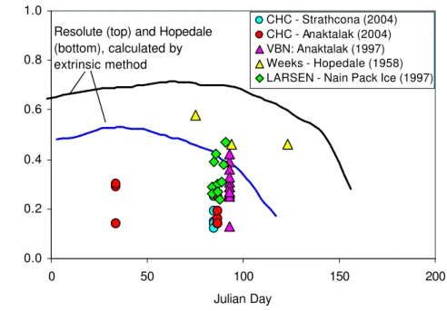
Ice property measurements from the above-mentioned sources were used to calculate the flexural strength of the ice using the intrinsic method (individual data markers shown in Figure 8). Measurements from Hebron Fjord (Gow, 1987) were not included in the figure because air and ice temperatures were not provided. Two solid lines were used to show the calculated flexural strengths for first-year ice at Hopedale and Resolute, calculated by the extrinsic method using the smoothed 30-yr MDT and mean ice thickness data. Plotting the flexural strength versus Julian Day resulted in a considerable amount of scatter, partly because the comparison does not allow for inter-annual variability in air temperatures.

0.0 0.2 0.4 0.6 0.8 1.0 0 50 100 150 200 Julian Day

CHC - Strathcona (2004) CHC - Anaktalak (2004) VBN: Anaktalak (1997) Weeks - Hopedale (1958) LARSEN - Nain Pack Ice (1997)

Resolute (top) and Hopedale (bottom), calculated by extrinsic method

Figure 8 Calculated flexural strength, expressed in terms of Julian Day

(flexural strength calculated using extrinsic method – solid lines; intrinsic method –data markers)

Realizing that some of the scatter in Figure 8 resulted from inter-annual variability in air temperatures, the calculated flexural strength was plotted directly as a function of air temperature (Figure 9). Although plotting the results in this manner eliminated some of the scatter, there continues to be considerable variability in the flexural strengths for the same study

area at the same air temperature (see the data markers for VBN and CHC). Results show that

fluctuations in air temperature do not entirely explain the variability in flexural strengths observed in Figure 9. Although the calculated flexural strength of the ice decreased with increasing air temperature, there is no clear correlation between the two parameters.

(25)

0.0 0.2 0.4 0.6 0.8 1.0 -30 -25 -20 -15 -10 -5 0 5 10

Measured air temperature (°C)

CHC - Anaktalak (2004) CHC - Strathcona (2004) VBN - Anaktalak (2004) LARSEN - Nain Pack (1997) Weeks - Hopedale (1958) Resolute (top) and Hopedale

(bottom), calculated by extrinsic method

Figure 9 Calculated flexural strength, expressed in terms of air temperature

(data points – intrinsic method; solid lines – extrinsic method)

Since ice strength is directly related to ice temperature, the calculated strengths were plotted against bulk ice temperatures. For comparison purposes, previous measurements of the ice borehole strength of Arctic ice were plotted in the same figure. Results are shown in Figure 10, where the ice borehole strength is shown on the left axis (square data markers) and the calculated flexural strength is shown on the right axis. Results from Gow (1987) and Weeks and Lee (1958) are not included in the figure because the authors did not give information about ice temperatures.

Figure 10 shows that a direct correlation exists between the bulk ice temperature and ice strength. The ice borehole strength is particularly important in this regard - it is affected by, but measured independently of, the ice temperature. The same is not true for the calculated flexural strengths, since the bulk ice temperature was one of the input parameters required for the calculation. Results show that it is preferable to relate the ice strength to the bulk (depth-averaged) ice temperature directly rather than to some derivative of the air temperature.

(26)

0 5 10 15 20 25 30 35 -20 -15 -10 -5 0

bulk ice temperature (°C)

Ice borehole strength (MPa)

0 0.2 0.4 0.6 0.8 1

BHS - Arctic (CHC) BHS - Arctic (literature) FS - Labrador (CHC) FS - Labrador (VBN) FS - Arctic (CHC) FS- Pack (LARSEN)

Figure 10 Ice borehole strength and flexural strength versus bulk ice temperature

(flexural strength (FS) was calculated using intrinsic method, using ice property measurements and borehole strength (BHS) was measured on level Arctic first-year ice)

7.0 Ice Strength Charts: Expressing Seasonal Changes in Strength

The ice strength algorithm for landfast first-year ice in the high Arctic used an exponential relation between the normalized ice strength and accumulated degree-days (Johnston and Timco, 2003-a). The strength output from the algorithm, and displayed on the preliminary Ice Strength Charts, was normalized to the maximum mid-winter flexural strength of Arctic first-year ice (0.71 MPa). Developing a specific algorithm for one location was considered appropriate for the high Arctic since it was based upon good agreement between the normalized flexural strength and the accumulated degree days. That methodology however, needed to be re-evaluated when considering ice at different latitudes.

7.1 Approaches for Displaying Strength on the Ice Strength Charts

Three different approaches were used to determine the most effective means of expressing the seasonal decrease in ice strength at different latitudes. The three approaches and their results are discussed below.

Case (i) - Ice Strength Normalized by mid-Winter Maximum of Arctic Ice Figure 11 shows the results of normalizing flexural strengths at different sites by the maximum mid-winter strength of Arctic first-year ice (0.71 MPa). Although this technique was appropriate for the strength algorithm developed for the high Arctic, it is not useful for ice outside the Arctic. One reason

(27)

for this is that many commercial vessels may not have experience with Arctic first-year ice. Normalizing the ice strength by some unfamiliar value would be irrelevant and would likely lead to confusion. 0.0 0.2 0.4 0.6 0.8 1.0 0 50 100 150 200 Julian Day

Flexural strength, normalized to maximum

Arctic strength Resolute

Chesterfield Churchill Hopedale Moosonee

Figure 11 Flexural strength, normalized by mid-winter strength of Arctic ice

Case (ii) - Ice Strength Normalized by Site-Specific Maximum Using this approach, the strength at the different sites would be normalized by the maximum ice strength that occurs for that area. Based upon flexural strengths calculated using smoothed 30-yr MDT and mean ice thicknesseses, the following peak strengths would be used at the different sites:

Moosonee - 0.52 MPa Hopedale - 0.53 MPa Churchill - 0.63 MPa Chesterfield - 0.67 MPa Resolute - 0.71 MPa

This procedure is not recommended because it removes differences in ice strength for each site (Figure 12). In effect, normalizing by the site-specific maximum is misleading, since it gives the impression that there is little difference between the strength of first-year ice at the different latitudes. The variation in ice strength with latitude should be preserved.

(28)

0.0 0.2 0.4 0.6 0.8 1.0 0 50 100 150 200 Julian Day

Flexural strength, normalized to site

maximum Resolute Chesterfield Churchill Hopedale Moosonee

Figure 12 Flexural strength, normalized by maximum strength at each site

Case (iii) - Ice Strength Expressed in terms of its Physical Units Using physical units for the Ice Strength Charts has the advantage that it allows the end user to become familiar with a bona fide ice strength, rather than the dimensionless value that results from normalizing (Figure 13). In addition, it preserves differences in strength that are characteristic of ice at different latitudes.

0.0 0.2 0.4 0.6 0.8 1.0 0 50 100 150 200 Julian Day

Resolute Chesterfield Churchill Hopedale Moosonee

(29)

7.2 Relating Ice Strength to ADD

The strength algorithm that was developed for Arctic ice related the decrease in ice strength to the accumulated degree-days (ADD). That required two steps – (i) selecting an appropriate start date from which to begin accumulating degree days and (ii) establishing a baseline from which to reference accumulating degree days. A start date of March 1 and a baseline temperature of – 30oC were appropriate for the high Arctic (Johnston and Timco, 2003-a).

The process of selecting a start date and baseline temperature for regions outside the Arctic made using the same approach for various regions extremely difficult. For example, a baseline of –35oC and a start date of January 1 would be needed to completely capture seasonal increases in temperature at all five selected sites. That procedure resulted in well-behaved curves when plotting accumulating degree days against Julian Day (Figure 14) but resulted in incoherent curves when the flexural strength was plotted against accumulated degree days (Figure 15).

0 1000 2000 3000 4000 5000 6000 0 50 100 150 200 Julian Day

ADD (deg days from -35°C on JD01)

Figure 14 Accumulated degree-days from baseline of -35°C and start date of January 1

Using the same start date and baseline temperature for all five sites mistakenly indicated that ice in the Arctic (Resolute, Chesterfield, Churchill) began decreasing in strength earlier and at a much steeper rate than ice at southern latitudes. Based upon the relation between ice strength and ice temperature (illustrated in Figure 10), thinner ice in the sub-Arctic should decrease in strength sooner (and likely at a faster rate) than in the Arctic. Figure 15 shows the opposite trend, which illustrates why the decrease in ice strength should not be related to ADD. That is not a rational approach for comparing ice strengths at different latitudes.

(30)

0 0.1 0.2 0.3 0.4 0.5 0.6 0.7 0.8 0 500 1000 1500 2000 2500 3000

ADD above -35°C from JD01

Figure 15 Seasonal decrease in ice strength as function of accumulated degree days

7.3 Charts Based upon the Flexural Strength Calculated Directly

The above discussion showed that relating the flexural strength to the accumulated degree days, based upon a standardized or flexible start date and baseline temperature, would not be appropriate for describing the decrease in strength that characterizes both sub-Arctic and Arctic ice. Rather, it is suggested that the flexural strength of the ice from different regions be calculated directly using the method developed by Timco and O’Brien (1994), as discussed below.

7.3.1 Extrinsic Method of Calculating the Flexural Strength: Equations

Since depth profiles of the ice temperature and ice salinity will not be available for all sites at all times, it will be necessary to calculate those parameters indirectly using known air temperatures (T_air) and estimated ice thicknesses (h_i). The air temperature and ice thickness will be used to calculate (a) S the bulk ice salinity, (b) T_surface the ice surface temperature, (c) T_ice a bulk ice temperature, (d) Vb a brine volume and (e) FS the flexural strength of the ice, as outlined in

the following equations. Salinity (ppt), S

for h_i < 0.34 m for h_i > 0.34 m

(31)

Ice surface temperature ( C), T_i-surface

for T_air < -10oC for T_air < -10oC

T_i-surface = 0.6 (T_air) – 4 T_i-surface = T_air

Bulk ice temperature (oC), T_ice

T_ice = (T_i-surface - 1.8)/2

Brine volume (ppt), Vb

for T_ice < -2.0oC for T_ice > -2.0oC

Vb = S ((49.185/ABS(T_ice)) + 0.532) Vb = 10000000000000

Flexural strength (MPa), FS

FS = 1.76 (exp(-5.88(sqrt(Vb/1000))

Table 3 showed that the extrinsic method of calculating the flexural strength from air temperature and estimated ice thickness data allows the ice strength at Moosonee to be determined until about the second week of April, and until the first week of June at Resolute. After that, the brine volume equation breaks down and the ice borehole strength must be used to document the seasonal decrease in ice strength. Since it has been suggested that the ice strength no longer be normalized, or related to the ADD, the borehole strength will need to be related to the flexural strength of the ice. That will require further study.

7.3.2 Effect of using MDT in Calculations

Determining the flexural strength from mean daily air temperatures requires making a decision about whether the mean daily temperatures (MDT) or a running average of the mean daily temperatures be used in the calculation. Figure 16 shows a comparison of the mean daily air temperatures for Resolute during 2002, the 7-day average of the 2002 mean daily temperatures and the two-week smoothed 30-yr mean daily temperatures. As might be expected, the 30-yr MDT all but eliminates day-to-day fluctuations in mean daily temperatures.

Figure 17 shows the effect of using the 2002 mean daily temperatures in the calculations – daily fluctuations in air temperature, although attenuated, are reflected in the calculated ice strength. Presently, there is little information about how quickly the ice responds to changes in air temperatures and the effect that it has on the ice strength. In order to determine whether the mean daily air temperature (or some average of it) should be used to calculate the flexural strength, work will need to be conducted on how quickly the ice responds to fluctuations in air temperature, and to what ice depth those changes occur. It is probable that, because of its thickness, Arctic first-year ice responds more slowly to those changes than sub-Arctic ice. The effect of an overlying snow cover will also factor in to the response time of the ice.

(32)

-50 -40 -30 -20 -10 0 10 0 50 100 150 200 Julian Day (JD)

Mean daily air temperature

2002 MDT 7 day 2002 MDT smoothed 30-yr MDT Resolute

Figure 16 2002 MDT, 7-day ave of 2002 MDT and the 2-week smoothed 30-yr MDT

0.00 0.20 0.40 0.60 0.80 1.00 0 50 100 150 200 Julian Day (JD) F

lexural strength (MPa)

Resolute - calculated using 2002 MDT

(33)

7.4 Mapping Ice Strength

The regional flexural strengths plotted in Figure 7 were overlaid on a map twice each month from February to May, as shown in Figure 18. The strength map provides a means of visualizing the spatial variability in ice strength and the type of strength contours that future Ice Strength Charts might show. The bi-monthly strengths are listed in Table 4.

Figure 18 and Table 4 include data for the period over which the Timco and O’Brien technique is valid. Obtaining strength data beyond that point would require conducting borehole strength tests. Those data, although already available for the high Arctic, will soon be available for landfast first-year ice along the Labrador Coast. Results have shown that the ice borehole strength and flexural strength complement one another very well, since both exhibit similar seasonal decreases in strength. A relation between the two different strengths needs to be developed before one of the strengths, or both, can be used as a basis for future Ice Strength Charts.

Table 4 Bi-monthly Calculated Flexural Strengths for Selected Sites

Date JD Resolute Chesterfield Churchill Hopedale/Nain Moosonee

Feb 8 39 0.69 0.67 0.63 0.53 0.51 Feb 20 51 0.71 0.68 0.63 0.51 0.48 Mar 6 66 0.71 0.66 0.61 0.48 0.45 Mar 21 81 0.70 0.64 0.59 0.44 0.39 Apr 5 96 0.69 0.61 0.54 0.37 0.28 Apr 17 108 0.65 0.57 0.46 0.26 -- May 2 123 0.60 0.51 0.30 -- -- May 14 135 0.54 0.39 -- -- -- May 29 150 0.39 -- -- -- -- June 14 165 -- -- -- -- --

(34)

Resolute 0.69 / 0.71 MPa Chesterfield 0.67 / 0.68 MPa Churchill 0.63 / 0.63 MPa Moosonee 0.51 / 0.48 MPa Nain 0.53 / 0.51 MPa Feb 8 / Feb 23 Resolute 0.71 / 0.70 MPa Chesterfield 0.66 / 0.64 MPa Churchill 0.61 / 0.59 MPa Moosonee 0.45 / 0.39 MPa Nain 0.48 / 0.44 MPa Mar 7 / Mar 22

(a) February (b) March

Resolute 0.69 / 0.65 MPa Chesterfield 0.61 / 0.57 MPa Churchill 0.54 / 0.46 MPa Moosonee 0.28 MPa / NA Nain 0.37 / 0.26 MPa Apr 6 / Apr 18 Resolute 0.60 / 0.54 MPa Chesterfield 0.51 / 0.39 MPa Churchill 0.30 MPa / NA Moosonee NA/ NA Nain NA / NA May 3 / May 15 (c) April (d) May Resolute 0.39 MPa / NA Chesterfield NA / NA Churchill NA / NA Moosonee NA / NA Nain NA / NA May 30 / Jun 14

(e) May and June

(35)

8.0 Conclusions

This report summarized the work that has been done on developing a methodology for including level, landfast first-year ice in the sub-Arctic into the Ice Strength Charts issued by CIS. Previously, Ice Strength Charts only encompassed the high Arctic therefore a considerable amount of work was needed before a feasible approach for incorporating sub-Arctic ice into the Strength Charts could be determined.

Past Ice Strength Charts were issued from May to August and were based upon normalizing the calculated flexural strength of the ice and the measured ice borehole strength by their mid-winter maximums (Johnston and Timco, 2003-a). The calculated flexural strength was normalized by 0.71 MPa and the borehole strength was normalized by a value of 29 MPa – values that corresponded to the maximum strengths of Arctic first-year ice in mid-winter. This study showed that basing Strength Charts on a normalized ice strength would not be appropriate when incorporating both Arctic and sub-Arctic areas in the Charts. The problem related to selecting appropriate values by which to normalize the flexural and borehole ice strengths, since whatever normalizing factors were selected would not have been appropriate for ice in all regions. Nor will that value be familiar to all Commanding Officers, since the ships operate in very different ice conditions. It is suggested that if future Ice Strength Charts are to incorporate sub-Arctic ice, ice strengths have physical units (kPa or MPa).

The Ice Strength Algorithm for the high Arctic related the normalized ice strength to a derivative of the air temperature, the accumulated degree days, with respect to a pre-determined baseline. That baseline was selected with the objective of completely capturing the seasonal warming of the ice, while minimizing the effect that subzero air temperatures had on the accumulating degree days for each area. The selected baseline temperature was used to determine the number of accumulated degree days that corresponded to the date on which the ice strength had been measured (or calculated). The ice strength was then plotted against the accumulated degree days, and the relation between the two parameters was described using an exponential equation – the so-called Ice Strength Algorithm.

This study showed that neither the previously developed Strength Algorithm nor the technique used to obtain it, were appropriate for comparing ice strengths at different latitudes. In fact, the premises that were used to develop a Strength Algorithm for the high Arctic (relating the ice strength to the accumulated degree days) led to misleading results when the same technique was applied to sites at other latitudes. Relating the strength to the accumulated degree days erroneously implied that Arctic ice decreased in strength before sub-Arctic ice. It was concluded that Ice Strength Charts for Arctic and sub-Arctic ice should rely upon direct calculations of the flexural strength of the ice, using the Timco and O’Brien (1994) technique.

Timco and O’Brien (1994) describe two approaches for calculating the flexural strength of the ice. The first, more accurate, approach uses the measured ice temperature and salinity. The second approach uses known information about the air temperature and ice thickness. Since it is not always possible, or practical, to measure the properties of ice, it is suggested that the Ice Strength Charts use flexural strengths calculated by the second technique (from air temperatures and estimated ice thicknesses).

(36)

The suggestion that future Ice Strength Charts display the flexural strengths that retain their physical units would be feasible up to a certain date. As the ice decays, its temperature and brine volume increase. Both approaches developed by Timco and O’Brien (1994) are valid until the square root of the brine fraction exceeds 0.5. Once that happens, the equations break down and the flexural strength can no longer be calculated. Herein lies the usefulness of the borehole jack: it can be used to measure ice strength when the flexural strength cannot be calculated. Past work has shown that, where there is data overlap, the flexural strength and the ice borehole strength show similar seasonal decreases.

Having data on the borehole strength of ice in the Arctic enabled CIS to construct Ice Strength Charts for the high Arctic after mid-June, when the flexural strength could no longer be calculated. To date, borehole strengths have only been measured on decaying first-year ice in the high Arctic. Results will soon be available from borehole strength tests that were recently conducted in landfast first-year ice off the Labrador coast. Year two of this project will use the knowledge gained from the Labrador ice to infer ice conditions in Hudson Bay and to determine whether sub-Arctic ice shows the same trend of decreasing strength observed in Arctic ice. Since it is suggested that future Ice Strength Charts calculate the ice strength directly using known air temperatures and estimated ice thickness, using the borehole jack as a proxy for the decrease in ice strength will require developing a direct relation between the flexural strength and the borehole strength of the ice. To date, no such relation has been developed. However, work has been done to relate the ice borehole strength to the confined compressive strength of ice that was measured in a laboratory (Sinha, 1986) and to the ice strength measured during unconfined compression tests (Masterson, 1996; Sinha, 1986).

This study showed a direct relation between measured ice borehole strength and the measured bulk ice temperature (depth-averaged). Similar results were obtained when the calculated flexural strength was plotted against the bulk ice temperature3. Using the bulk ice temperature to indicate ice strength underscores the importance of relating known air temperatures to bulk ice temperatures. This ‘not-so-straightforward’ relation becomes even more complicated when a dry or wet snow cover blankets the ice. Timco and O’Brien (1994) make assumptions about the effect that an overlying snow cover has in attenuating temperature changes in the ice, however this is an area that deserves further attention. This is especially true considering that the snow cover in sub-Arctic regions experiences changes almost daily, unlike the relatively stable snow pack in the Arctic. As a first approach, the technique developed by Timco and O’Brien (1994) can be used to calculate the flexural strength, however the influence that snow has on the ice temperature (hence ice strength) should be examined.

If future Strength Charts are to use air temperatures to calculate the flexural strength of the ice, a decision should be made as to which type of averaging would be appropriate for the air temperatures output by CIS’s GEM model. In this report, the two-week smoothed average of the 30-year normal mean daily temperatures (MDT) were used to calculate the flexural strength of the ice. Results showed these air temperatures do not have the regional, interannual

3

The two variables were not independent of one another, however, since ice temperature was an input for the calculations.

(37)

variability although, at present, it is not known how much that variability affects ice strength, in the short term. Before an air temperature is selected for strength calculations, attention should be given to examining the response time of the ice to changes in air temperature, and how those temperature changes affect its ice strength. Once that has been done, it would be possible to select the air temperature that is most appropriate for calculating the flexural strength of the ice. This study focused upon developing a technique for incorporating level, landfast first-year ice in the sub-Arctic into future Ice Strength Charts. The properties of decaying landfast ice in the Arctic have been measured for three years and, after this year, will have been measured for one year in the sub-Arctic. It would be of interest to relate measurements of landfast first-year ice to measurements made in pack ice. Work is currently being performed in rubbled ice off Labrador. Those results could be used to understand how the properties of first-year ice embedded in pack ice differs from landfast ice.

9.0 Summary

A number of suggestions about incorporating sub-Arctic ice into future Ice Strength Charts were put forth. The study also recommended areas in which future work should be directed to enhance understanding of how the ice responds to environmental changes and the impact that those changes have on ice strength. That information would lead to improved Ice Strength Charts. The suggestions are summarized below:

• If the Ice Strength Charts are to incorporate sub-Arctic ice, the ice strength should be expressed in physical units rather than normalized by a maximum strength.

• Ice Strength Charts that include Arctic and sub-Arctic ice should rely upon direct calculations of the flexural strength using the Timco and O’Brien (1994) approach. That requires data on air temperatures and estimated ice thicknesses.

• Using the ice borehole strength as a proxy for the flexural strength (beyond where it can be calculated) requires developing a direct relation between the two strengths.

• The influence that snow cover has on the bulk ice temperature, hence ice strength, is very important and should be examined.

• Attention should be given to quantifying the response time of the ice to short term changes in air temperature, and its implications for ice strength.

• A first look at relating the properties of landfast first-year ice to first-year ice in the transition zone is possible using recently acquired data on rubbled ice off the Labrador Coast.

(38)

10.0 Acknowledgments

Financial support for this project was provided by Canadian Ice Service. That assistance is most appreciated. Transport Canada and Canadian Ice Service sponsored the field program that was conducted in the landfast ice off the Labrador Coast. Many thanks to both departments for their continued support and interest in this area.

11.0 References

Bilello, M.A. (1960) Formation, Growth and Decay of Sea Ice in the Canadian Arctic Archipelago. U.S. Army Snow Ice and Permafrost Research Establishment Corps of Engineers. Research Report 65

Bilello, M.A. (1980) Maximum Thickness and Subsequent Decay of Lake, River and Fast Sea Ice in Canada and Alaska. U.S. Army Cold Regions Research and Engineering Laboratory, Hanover, New Hampshire.

Bilello, M.A. and Lunardini, V.J. (1996) Ice Thickness Observations, North American Arctic and Subarctic, 1974 – 75, 1975 – 76 and 1976 – 77. CRREL Special Report. No. 43, IX. May, 1996. 221 pp.

Bilello, M.A. and R.E. Bates (1991) Ice Thickness Observations: North American Arctic and Subarctic, 1972-73 and 1973-74. Special Report 43, VIII. U.S. Army Cold Regions Research and Engineering Laboratory, Hanover, New Hampshire.

Cormorant Ltd. (1997) Voisey’s Bay Ice Monitoring Program: Program Report. Prepared for Voisey’s Bay Nickel Company Limited, St. John’s, Newfoundland.

Gow, A.J. (1987) Crystal structure and salinity of sea ice in Hebron Fiord and vicinity, Labrador. U.S. Army Cold Regions Research and Engineering Laboratory, Hanover, New Hampshire.

Johnston, M., Frederking, R. and Timco, G. (2002) Properties of Decaying First Year Sea Ice: Two Seasons of Field of Field Measurements. Proceedings 17th International on Okhotsk Sea and Sea Ice, Mombetsu, Hokkaido, Japan, pp. 303-311.

Johnston, M. and Timco, G. (2003-a) Developing an Ice Strength Algorithm for Level, Landfast First-year ice in the High Arctic. Technical report issued by Canadian Hydraulics Centre for Canadian Ice Service, March 2003, Ottawa, Ontario, CHC-TR-013, 21 p.

Johnston, M., Frederking, R. and Timco, G. (2003-b) Properties of Decaying First-year Sea Ice at Five Sites in Parry Channel. Proceedings 17th International Conference on Port and Ocean Engineering under Arctic Conditions, POAC’03, Trondheim, Norway, Vol. 1, pp. 131-140. Kirby, C. (1997) Voisey’s Bay Ice Probe 1997 on CCGS HENRY LARSEN. Report issued by

Institute for Marine Dynamics of the National Research Council, submitted to the Canadian Coast Guard, TR-1997-26, September, 1997, 9 p.

Masterson, D. (1996) Interpretation of In Situ Borehole Ice Strength Measurement Tests. Can.

(39)

Sinha, N. K. (1986) The Borehole Jack: Is it a Useful Tool? Proc. of 5th Int. Offshore Mechanics and Arctic Engineering Symp. (OMAE). Tokyo, Japan. 13 – 17 April 1986. Vol. IV. pp. 328 – 335.

Timco, G. and Frederking, R. (1990) Compressive Strength of Sea Ice Sheets. Cold Regions Science and Technology, No. 17, pp. 227 - 240.

Timco, G. and O'Brien, S. (1994) Flexural Strength Equation for Sea Ice. Jour. Cold Regions Science and Technology, Vol. 22, pp. 285 – 298.

Weeks, W.F. and Lee, O.S. (1958). Observations on the Physical Properties of Sea-Ice at Hopedale, Labrador. Arctic, Vol. 11(3), pp. 135-155. September 1958. Canada.

(40)

(41)

(42)

REFERENCES

1. Barber, F.G and M.M. Larnder (1968). The Water and Ice of Hudson Bay. in Science, History and Hudson Bay Vol. 1 Edited by C.S. Beals, pp. 318-341. Dept of Energy, Mines and Resources, Ottawa.

2. Belliveau, D.J., C.L. Tang, and A.M. Mahon (1998). Measurement of Ice Growth and Melt in the Labrador Pack Ice. Proceedings of the Eighth (1998) International Offshore and Polar Engineering Conference, Vol. 3, pp. 36-41. Montreal, Canada, May 24-29, 1998.

3. Berenger, D. and B.D. Wright (1980). Ice Conditions Affecting Offshore Hydrocarbon Production in the Labrador Sea. Intermaritec 80 Int. Conference on Marine Sciences and Ocean Engineering. IMT 80-203 Hamburg

4. Bilello, M.A. (1960). Formation, Growth and Decay of Sea Ice in the Canadian Arctic Archipelago. U.S. Army Snow Ice and Permafrost Research Establishment Corps of Engineers. Research Report 65.

5. Bilello, M.A. (1980). Maximum Thickness and Subsequent Decay of Lake, River and Fast Sea Ice in Canada and Alaska. U.S. Army Cold Regions Research and Engineering Laboratory, Hanover, New Hampshire.

6. Bilello, M.A. and R.E. Bates (1991). Ice Thickness Observations: North American Arctic and Subarctic, 1972-73 and 1973-74. Special Report 43, VIII. U.S. Army Cold Regions Research and Engineering Laboratory, Hanover, New Hampshire.

7. Canadian Coast Guard (1998). Final Report: Voisey’s Bay Ice Probe. March.

8. Carsey, F.D., S.A. Digby Argus, M.J. Collins, B. Holt, C.E. Livingstone and C.L. Tang (1989). Overview of LIMEX'87 Ice Observations. IEEE Transactions on Geoscience and Remote Sensing, Vol. 27, No. 5, September 1989.

9. Catchpole, A.J.W. and M.-A. Faurer (1983). Summer Sea Ice Severity in Hudson Strait, 1751-1870. Climatic Change Vol. 5 (2) pp. 115-139.

10. Centre for Cold Ocean Resources Engineering (1977). Meteorological Ground Truthing, Hopedale. Field Data Report No. 5. C-CORE Publication 77-34.

11. Centre for Cold Ocean Resources Engineering (1977). Ice Characterization, Hopedale. Field Data Report No. 6. C-CORE Publication 77-35.

12. Centre for Cold Ocean Resources Engineering (1977). Additional Ground Truth Measurements, Hopedale. Field Data Report No. 7. C-CORE Publication 77-36.

13. Centre for Cold Ocean Resources Engineering (1977). Ground Truth Measurements, Goose Bay. C-CORE Field Data Report No.9. Publication 77-38.

14. Centre for Cold Ocean Resources Engineering (1979). Project SAR ’77 Summary Report. C-CORE Publication 79-15.

15. Cormorant Ltd. (1997). Voisey’s Bay Ice Monitoring Program: Program Report. Prepared for Voisey’s Bay Nickel Company Limited, St. John’s, Newfoundland.

16. Cormorant Ltd. (1998). Voisey’s Bay Ice Monitoring Program: Component Project Data Report 1. Landfast Ice Thickness Measurements Along the Voisey’s Bay Potential Shipping Route. Prepared for Voisey’s Bay Nickel Company Limited, St. John’s, Newfoundland. 3 August 1998.

17. Danielson, E.W. (1971). Hudson Bay Ice Conditions, Arctic 27 (2), pp. 90-106.

18. DF Dickens Associates Ltd. (1997). Review of Historical Ice Conditions Affecting the Voisey’s Bay Development. Prepared for Voisey’s Bay Nickel Company Limited, St. John’s, Newfoundland.

(43)

19. DF Dickens Associates Ltd. (1997). Voisey’s Bay 1996 Environmental Baseline Technical Data Report: Spring Ice Break-Up Survey. Prepared for Voisey’s Bay Nickel Company Limited, St. John’s, Newfoundland.

20. Environment Canada (1974). Ice summary and analysis 1971 Hudson Bay and approaches 43 p.

21. FENCO (1977). Winter Field Ice Survey Offshore Labrador, 1977. Prepared for TOTAL Eastcan Exploration Ltd, Calgary, Alberta.

22. Freeman, N.G., J.C. Roff, and R.J. Pett (1982). Physical, chemical and biological features of river plumes under an ice cover in James and Hudson's Bays. Nat. Can. Que., 109, pp. 745-764.

23. Godin, G. (1986). Modification by an ice cover of the tide in James Bay and Hudson Bay. Arctic, 39: p 65-67.

24. Gow, A.J. (1987). Crystal structure and salinity of sea ice in Hebron Fiord and vicinity, Labrador. U.S. Army Cold Regions Research and Engineering Laboratory, Hanover, New Hampshire.

25. Ingram, R.G. and P. Larouche (1987). Variability of an under-ice river plume. J. Geophys. Res. 92, pp. 9541-9547.

26. Langleben, M.P. (1959) Some Physical Properties of Sea Ice II. Can. J. Phys. Vol. 37. 27. Langleben, M.P. (1972) Decay of an annual cover of sea ice. Journal of Glaciology,

11(63), p 337- 344.

28. Larnder, M.M. (1968). The ice. in Science, History and Hudson Bay, Part 1, edited by C.S. Beals, pp. 318-341. Dept of Energy, Mines and Resources, Ottawa.

29. Larouche, P. and P.S. Galbraith (1989). Factors Affecting Fast-Ice Consolidation in Southeastern Hudson Bay, Canada. Atmosphere-Ocean, Vol. 27 (2), pp. 367-375. Canadian Meteorological and Oceanographic Society.

30. LeDrew, B.R. and S.T. Culshaw (1977). Ship-in-the-Ice Data Report. Centre for Cold Ocean Resources Engineering, St. John’s, Canada. C-CORE Publication No. 77-28. 31. Lepage, S. and R.G. Ingram (1991). Variation of Upper Layer Dynamics During

Breakup of the Seasonal Ice Cover in Hudson Bay. Journal of Geophysical Research, Vol. 96, No. C7, pp. 12,711- 12,724, July 15, 1991.

32. Loset, S., A. Langeland, B. Bergheim & K.V. Hoyland (1998). Geometry and physical properties of a stamucha found on Spitsbergen. Proceedings of the 14th International Symposium on Ice (IAHR), Vol. 1, pp. 339-344. July 27-31, 1998.

33. Martinson, C.R. (1985). Impulse radar sounding of level first-year sea ice from an icebreaker. U.S. Army Cold Regions Research and Engineering Laboratory, Hanover, New Hampshire.

34. McKenna, R. L. (1989). Section 8.7: Ice Mechanical Properties. LIMEX’89 Data Report. Energy, Mines and Resources Canada.

35. Moore, B.D.H. and A.F. Gregory (1979). Monitoring and Mapping Sea-Ice Breakup and Freezeup of Arctic Canada from Satellite Imagery. Arctic and Alpine Research, Vol. 11(2), pp. 229-242.

36. Peterson, I.K. (1990). Sea ice velocity fields off Labrador and eastern Newfoundland derived from satellite imagery: 1984-1987. Can. Tech. Rep. Hydrogr. Ocean Sci. No. 129:vi, 85 p.

37. Pounder, E. R. and E. M. Little (1959). Some Physical Properties of Sea Ice I. Can. J. Phys. Vol. 37.

(44)

38. Prinsenberg, S.J. (1980). Man-made changes in the freshwater input rates of Hudson and James Bays. Can. J. Fish. Aquat. Sci., Vol. 37, pp. 1101-1110.

39. Prinsenberg, S.J. (1986). Man-made changes in the freshwater input rates of Hudson and James Bays. in Canadian Inland Seas by I.P. Martini, pp. 163-186.

40. Prinsenberg, S.J. (1987). Seasonal Current Variations Observed in Western Hudson Bay. Journal of Geophysical Research, Vol. 92, No. C10, pp. 10756-10766, September 15, 1987.

41. Prinsenberg, S.J. (1988). Ice-cover and ice-ridge contributions to the freshwater contents of Hudson Bay and Foxe Basin. Arctic, Vol. 41, pp. 6-11.

42. Prinsenberg, S.J. and I.K. Peterson (1992). Sea-Ice Properties off Labrador and Newfoundland During LIMEX '89. Atmosphere-Ocean, Vol. 30 (2), pp. 207-222. Canadian Meteorological and Oceanographic Society.

43. Raney, R.K., S. Digby Argus and L. NcNutt (1989). Labrador Ice Margin Experiment LIMEX’89; An Overview. IGARSS Int. Geosci. and Remote Sensing Symp. Vol. 3 Part 3, p 1517-1519.

44. Rescan Environmental Services Limited (1997). Physical Oceanography of the Voisey’s Bay Project Area- Voisey’s Bay Nickel Company Environmental Impact Assessment. Prepared for Voisey’s Bay Nickel Company Limited, St. John’s, Newfoundland. November 1997.

45. Steel, A., J.I. Clark and P. Morin (1994). A comparison of pressuremeter test results in sea ice. Canadian Geotechnical Journal, Vol. 31, No. 2, pp. 254-260.

46. Tan, F.C. and P.M. Strain (1996). Sea ice and oxygen isotopes in Foxe Basin, Hudson Bay and Hudson Strait, Canada. Journal of Geophysical Research, Vol. 101 (C9), pp. 20869-20876.

47. Transportation Development Centre (1985). Trials off the Labrador Coast May 1984, Transport Canada. Edited by: R. Frederking and J.E. Laframboise. Polarstern: Report from the Canadian Team. May 1985.

48. Veitch, B., P. Kujala, P. Kosloff and M. Lepparanta (1991). Field Measurements of the Thermodynamics of an Ice Ridge. Helsinki University of Technology, Faculty of Mechanical Engineering, Laboratory of Naval Architecture and Marine Engineering. 49. Wang, J., L.A. Mysak and R.G. Ingram (1994). Interannual Variability of Sea-Ice Cover

in Hudson Bay, Baffin Bay and Labrador Sea. Atmosphere Ocean, Vol. 32 (2) 1994, pp. 421-447. Canadian Meteorological and Oceanographic Society.

50. Weeks, W.F. and O.S. Lee (1958). Observations on the Physical Properties of Sea-Ice at Hopedale, Labrador. Arctic, Vol. 11(3), pp. 135-155. September 1958. Canada.

51. Winsor, W.D., G.B. Crocker, R.F. McKenna, and C.L. Tang (1990). Sea Ice Observations during LIMEX, March - April 1989. Canadian Data Report of Hydrography and Ocean Sciences No. 81: iv, 43 p.