Business-Cycle Anatomy
The MIT Faculty has made this article openly available.
Please share
how this access benefits you. Your story matters.
Citation
Angeletos, George-Marios et al. “Business-Cycle Anatomy.”
American Economic Review, 110, 10 (October 2020): 3030-3070 ©
2020 The Author(s)
As Published
10.1257/AER.20181174
Publisher
American Economic Association
Version
Final published version
Citable link
https://hdl.handle.net/1721.1/130273
Terms of Use
Article is made available in accordance with the publisher's
policy and may be subject to US copyright law. Please refer to the
publisher's site for terms of use.
3030
Business-Cycle Anatomy
†By George-Marios Angeletos, Fabrice Collard, and Harris Dellas*
We propose a new strategy for dissecting the macroeconomic time series, provide a template for the business-cycle propagation
mech-anism that best describes the data, and use its properties to appraise
models of both the parsimonious and the medium-scale variety. Our findings support the existence of a main business-cycle driver but rule out the following candidates for this role: technology or other shocks that map to TFP movements; news about future productivity; and inflationary demand shocks of the textbook type. Models aimed at accommodating demand-driven cycles without a strict reliance on nominal rigidity appear promising. (JEL C22, E10, E32)
One is led by the facts to conclude that, with respect to the qualitative behavior of comovements among series, business cycles are all alike. To theoretically inclined economists, this conclusion should be attractive and challenging, for it suggests the possibility of a unified explanation of busi-ness cycles.
—Lucas (1977)
In their quest to explain macroeconomic fluctuations, macroeconomists have often relied on models in which a single, recurrent shock acts as the main business-cycle driver.1 This practice is grounded not only on the desire to offer a
parsimonious, unifying explanation as suggested by Lucas, but also on the prop-erty that such a model may capture diverse business-cycle triggers if these share a common propagation mechanism: multiple shocks that produce similar impulse
1 Examples include the monetary shock in Lucas (1975), the TFP shock in Kydland and Prescott (1982), the
sunspot in Benhabib and Farmer (1994), the investment shock in Justiniano, Primiceri, and Tambalotti (2010), the risk shock in Christiano, Motto, and Rostagno (2014), and the confidence shock in Angeletos, Collard, and Dellas (2018).
* Angeletos: MIT Department of Economics (email: [email protected]); Collard: Toulouse School of Economics (CNRS) (email: fabrice.collard@ tse-fr.eu); Dellas: Department of Economics, University of Bern (email: harris. [email protected]). Mikhail Golosov was the coeditor for this article. A preliminary version of the empirical strategy of this paper appeared in Section II of Angeletos, Collard, and Dellas (2015); this earlier exploration is fully subsumed here. We thank the coeditor, Mikhail Golosov, and three anonymous referees for extensive feed-back. For useful comments, we also thank Fabio Canova, Larry Christiano, Patrick Fève, Francesco Furlanetto, Jordi Galí, Lars Hansen, Franck Portier, Juan Rubio-Ramirez, and participants at various seminars and conferences. Angeletos acknowledges the financial support of the National Science Foundation (Award #1757198). Collard acknowledges funding from the French National Research Agency (ANR) under the Investments for the Future program (Investissements d’Avenir, grant ANR-17-EURE-0010).
† Go to https://doi.org/10.1257/aer.20181174 to visit the article page for additional materials and author
responses for all variables of interest can be considered as essentially the same shock.2
Is there evidence of such a common propagation mechanism in macroeconomic data? And if yes, what does it look like?
We address these questions with the help of a new empirical strategy. The strat-egy involves taking multiple cuts of the data. Each cut corresponds to a structural vector autoregression (SVAR)-based shock that accounts for the maximal volatility of a particular variable over a particular frequency band. Whether these empirical objects have a true structural counterpart in the theory or not, their properties form a rich set of cross-variable, static and dynamic restrictions, which can inform macro-economic theory. We call this set the “anatomy.”
A core subset of the anatomy is the collection of the five shocks obtained by targeting the main macroeconomic quantities, namely unemployment, output, hours worked, consumption, and investment, over the business-cycle frequencies. These shocks turn out to be interchangeable in the sense of giving rise to nearly the same impulse response functions (IRFs) for all the variables, as well as being highly cor-related with one another.
The interchangeability of these empirical shocks supports parsimonious theories featuring a main, unifying, propagation mechanism. Their shared IRFs provide an empirical template of it.
In combination with other elements of our anatomy, this template rules out the following candidates for the main driver of the business cycle: technology or other shocks that map to TFP movements; news about future productivity; and inflation-ary demand shocks of the textbook type.
Prominent members of the dynamic stochastic general equilibrium (DSGE) liter-ature also lack the propagation mechanism seen in our anatomy of the data, despite their use of multiple shocks and flat Phillips curves and their good fit in other dimen-sions. The problem seems to lie in the flexible-price core of these models. Models that instead allow for demand-driven cycles without a strict reliance on nominal rigidity hold promise.3
A. The Empirical Strategy
We first estimate a VAR (or a vector error correction model (VECM)) on the fol-lowing ten macroeconomic variables over the 1955–2017 period: the unemployment rate; the per capita levels of GDP, investment (inclusive of consumer durables), consumption (of nondurables and services), and total hours worked; labor produc-tivity in the nonfarm business sector; utilization-adjusted total factor producproduc-tivity (TFP); the labor share; the inflation rate (GDP deflator); and the federal funds rate. We next compile a collection of shocks, each of which is identified by maximizing
2 To echo Cochrane (1994, p. 298): “The study of shocks and propagation mechanisms are of course not
sepa-rate enterprises. Shocks are only visible if we specify something about how they propagate to observable variables.”
3 Recent examples include Angeletos, Collard, and Dellas (2018); Angeletos and La’O (2010, 2013); Angeletos
and Lian (2020); Bai, Ríos-Rull, and Storesletten (2017); Beaudry and Portier (2014, 2018); Beaudry, Galizia, and Portier (2018); Benhabib, Wang, and Wen (2015); Eusepi and Preston (2015); Huo and Rios-Rull (forthcoming) ;Jaimovich and Rebelo (2009); Huo and Takayama (2015); and Ilut and Saijo (2018). Related is also the earlier literature on coordination failures (Diamond 1982, Benhabib and Farmer 1994, Guesnerie and Woodford 1993).
its contribution to the volatility of a particular variable over either business-cycle frequencies ( 6–32 quarters) or long-run frequencies (80– ∞ ). We finally inspect the empirical patterns encapsulated in each of these shocks, namely the implied IRFs and variance contributions.
This approach builds on the important work of Uhlig (2003). Our main contri-bution vis-à-vis this and other works that employ the so-called max-share identifi-cation strategy (Barsky and Sims 2011, Faust 1998, Neville et al. 2014) lies in the multitude of the one-dimensional cuts of the data considered, the empirical regular-ities thus recovered, and the novel lessons drawn for theory.4
An additional contribution is to clarify the mapping from the frequency domain to the time domain: we show that the shock that dominates the business-cycle fre-quencies ( 6–32 quarters) is a shock whose footprint in the time domain peaks within a year or two. In other words, targeting 6–32 quarters in the time domain does not recover the business cycle.
Our approach also departs from standard practice in the SVAR literature, which aims at identifying empirical counterparts to specific theoretical shocks (for a review, see Ramey 2016). Instead, it sheds light on dynamic comovements by tak-ing multiple cuts of the data, one per targeted variable and frequency band. These multiple cuts form a rich set of empirical restrictions that can discipline any theory, whether of the parsimonious type or the DSGE type.
B. The Main Business-Cycle Shock
Consider the shocks that target any of the following variables over the business-cycle frequencies: unemployment, hours worked, GDP, and investment. These shocks are interchangeable in terms of the dynamic comovements, or the IRFs, they produce. Furthermore, any one of them accounts for about three-quarters of the business-cycle volatility of the targeted variable and for more than one-half of the business-cycle volatility in the remaining variables, and also triggers strong positive comovement in all variables. In expanded specifications that include the output gap or the unemployment gap, the shocks identified by targeting any one of these gaps produce nearly identical patterns as well. Finally, the shock that targets consumption is less tightly connected in terms of variance contributions, but still similar in terms of dynamic comovements.
These findings offer support for theories featuring either a single, dominant, business-cycle shock, or multiple shocks that leave the same footprint because they share the same propagation mechanism. With this idea in mind, we use the term Main Business Cycle (MBC) shock to refer to the common empirical footprint, in terms of IRFs, of the aforementioned reduced-forms shocks. This provides the sought-after template for what the propagation mechanism should be in any “good” model of the business cycle.5
4 A detailed discussion of how our method and results differ from those of Uhlig (2003) and various other works
is offered in the next section.
5 As with any other filter that focuses on the business-cycle frequencies of the data, the use of our template for
model evaluation is of course based on the premise that business-cycle models ought to be evaluated by such a met-ric. This accords with a long tradition in macroeconomics. See, however, Canova (2020) for a contrarian view based on the property that the business-cycle and lower-frequency predictions of DSGE models are tightly tied together;
A central feature of this template is the interchangeability property, namely that all the aforementioned shocks produce essentially the same IRFs, or the same prop-agation mechanism. Below, we describe additional stylized facts revealed via our anatomy and discuss the overall lessons for theory. At first, we draw lessons through the perspective of single-shock models. Later, we switch to multishock models and discuss the challenges and the use of our method in such models.
C. Disconnect from TFP and from the Long Run
The MBC shock is disconnected from TFP at all frequencies. It also accounts for little of the long-term variation in output, investment, consumption, and labor pro-ductivity. Symmetrically, the shocks that have the maximal contribution to long-run volatility have a small contribution to the business cycle.
These findings challenge not only the baseline RBC model but also models that map other shocks, including financial, uncertainty, and sunspot shocks, into endog-enous TFP fluctuations. Benhabib and Farmer (1994); Bloom et al. (2018); and Bai, Ríos-Rull, and Storesletten (2017) are notable examples of such models. In these models, the productivity movements over the business-cycle frequencies ought to be tightly tied to the MBC shock, which is not the case.
These findings also challenge Beaudry and Portier (2006), Lorenzoni (2009), and other works that emphasize signals (news) of TFP and income in the medium to long run. If such news, noisy or not, were the main driver of the business cycle, the MBC shock would be a sufficient statistic of the available information about future TFP movements, which is hard to square with our findings. Instead, a semistructural exercise based on our anatomy suggests that the contribution of TFP news to unem-ployment fluctuations is in the order of 10 percent, which is broadly consistent with the estimate provided by Barsky and Sims (2011).
The MBC shock fits better the notion of an aggregate demand shock unrelated to productivity and the long run, in line with Blanchard and Quah (1989) and Galí (1999). However, as discussed below, this shock ought to be non-inflationary, which may or may not fit the New Keynesian framework.
D. Disconnect from Inflation
The shock that targets unemployment accounts for less than 10 percent of the fluctuations in inflation, and conversely the shock that targets inflation explains a small fraction of unemployment fluctuations. A similar disconnect obtains between inflation and the labor share, a common proxy of the real marginal cost in the New Keynesian framework (Galí and Gertler 1999), as well as between inflation and the output or unemployment gap.6 This challenges the interpretation of the MBC shock
as a demand shock of the textbook type.
and Beaudry, Galizia, and Portier (2020) for evidence suggestive of predictable boom-bust phenomena that operate at both business-cycle and medium-run frequencies.
6 This disconnect is stronger in the post-Volker period and echoes a large literature that documents, via other
meth-ods, the disappearance of the Phillips curve from the data (e.g., Atkeson and Ohanian 2001; Dotsey, Fujita, and Stark 2018; Mavroeidis, Plagborg-Møller, and Stock 2014; Stock and Watson 2007, 2009). McLeay and Tenreyro (2020)
Could this disconnect reflect the confounding effects of an inflationary demand shock and a disinflationary supply shock? The answer is negative if the supply shock in the theory is proxied by the shock that accounts for TFP or labor productivity in the data, or the demand shock is the main driver of the business cycle and the Phillips curve is not exceedingly flat.
This brings us to the topic of how this disconnect and the Keynesian view of demand-driven business cycles fit together in state-of-the-art DSGE models. First, a sufficiently accommodative monetary policy is used to overcome the Barro-King challenge (Barro and King 1984) and undo the negative comovement between employment and consumption induced by demand shocks in the flexible-price core of these models. Second, overly flat Phillips curves for both wages and prices are used to make sure that demand-driven fluctuations are nearly noninflationary. And third, the bulk of the observed inflation fluctuations is accounted by a residual.
Whether this interpretation of the macroeconomic data is consistent with micro-economic evidence on price and wage rigidity is the topic of a large, inconclu-sive literature that is beyond the scope of this paper. A different possibility is that demand-driven business cycles are not tied to nominal rigidity. Below we discuss how our anatomy of the macroeconomic data favors a model that accommodates this possibility.
E. The Anatomy of Medium-Scale DSGE Models
Our empirical strategy was motivated by parsimonious models. Does its retain its probing power in state-of-the-art, medium-scale DSGE models?
Such models pose a direct challenge for the interpretation and use of the identi-fied MBC shock, as this may correspond to a combination of multiple theoretical shocks, none of which individually has its properties.7 But at the same time, such
models give rise to a larger set of cross-variable, static, and dynamic restrictions that can be confronted with our multidimensional anatomy of the data.
We demonstrate these ideas in Section V using two off-the-self models. One is the sticky-price model of Justiniano, Primiceri, and Tambalotti (2010); this is essen-tially the same as that developed in Christiano, Eichenbaum, and Evans (2005) and Smets and Wouters (2007). Another one is the flexible-price model found in an earlier paper of ours, Angeletos, Collard, and Dellas (2018): this is an extension of the RBC model that allows business cycles to be driven by variation in “confidence” and “news about the short-run economic outlook.” We view the former as represen-tative of the New Keynesian paradigm and the latter as an example of a literature that aims at accommodating demand-driven business cycles without a strict reliance on nominal rigidity.
In each model, we perform an anatomy similar to that carried out in the data: we take different linear combinations of the theoretical shocks, each one constructed by
argues that this fact may reflect the conduct of monetary policy, rather than a problem with the true, structural Phillips curve. We discuss why our evidence challenges this view in Section IID.
7 This difficulty is not specific to our approach. It concerns any approach that requires a single shock to drive
some conditional variance in the data. For instance, Galí (1999) requires that a single shock drives productivity in the long run, an assumption inconsistent with the literature on news shocks.
maximizing the business-cycle volatility of a different variable. We then compare the model-based objects to their empirical counterparts.
Both of the aforementioned two models match the disconnect of the MBC shock from TFP and inflation. However, the first model has difficulty matching the inter-changeability property of the MBC template: the reduced-form shocks obtained by targeting the key macroeconomic quantities are less similar in the model than their empirical counterparts. This is because this model, like many other members of the DSGE literature, attributes the business cycle to a fortuitous combination of special-ized theoretical shocks, none of which generates the empirically relevant comove-ment patterns in the key macroeconomic quantities. By contrast, the second model fits the patterns seen in the data because it contains a dominant shock, or propaga-tion mechanism, that alone generates these patterns.
As an additional demonstration of the value of our method, we use it to evaluate the model of Christiano, Motto, and Rostagno (2014). This model is a leader in a new strand of the DSGE literature that includes financial frictions and uses finan-cial (risk) shocks to drive the business cycle. We find that this model, too, but to a smaller degree, is subject to the challenge discussed above. It also misses some of the dynamic patterns seen in the data between the MBC shock, the credit spread and the level of credit.
In both Justiniano, Primiceri, and Tambalotti (2010) and Christiano, Motto, and Rostagno (2014), a large part of the difficulty to match the empirical template we provide in this paper can be traced to their flexible-price core. Sticky prices, sticky wages, accommodative monetary policies, and various adjustment costs help amelio-rate the problem but do not really fix it. In our view, this hints again at the value of theories that aim at accommodating demand-driven cycle without a strict reliance on nominal rigidity. But even if one does not accept this conclusion, the conducted exer-cises illustrate the probing power of our empirical strategy for models of any size.
I. Data and Method
The data used in our main specification consist of quarterly observations on the following ten macroeconomic variables: the unemployment rate ( u ); the real, per capita levels of GDP ( Y ), investment ( I ), consumption ( C ); hours worked per person ( h ); labor productivity in the nonfarm business sector ( Y/h ); the level of utilization-adjusted total factor productivity (TFP); the labor share ( wh/Y ); the infla-tion rate ( π ), as measured by the rate of change in the GDP deflator; and the nominal interest rate ( R ), as measured by the federal funds rate. The sample starts in 1955:I, the earliest date of availability for the federal funds rate, and ends in 2017:IV.
Following standard practice, and to ensure compatibility with the models used in Section V, our investment measure includes consumer expenditure on durables, while our consumption measure consists of expenditure on nondurables and ser-vices. Both measures are deflated by the GDP deflator. Section IIIC establishes the robustness of our results to the use of component-specific deflators; to different samples, such as the pre- and post-Volcker periods or excluding the Great Recession and the ZLB period; and to the incorporation of additional information, such as that contained in stock prices and financial variables. Appendix Section A contains the definitions and data sources.
We now turn to the description of the empirical method. As mentioned in the intro-duction, the method involves running a VAR on the aforementioned ten variables and recovering certain “shocks.” As in the SVAR literature, any of the shocks con-structed here represents a particular linear combination of the VAR residuals. What distinguishes our approach is the criterion used in the identification of such a linear combination.
Let the VAR take the form
A
(
L)
X t = ν t ,where the following definitions apply: X t is an N × 1 vector, containing the mac-roeconomic variables under consideration; A
(
L)
≡ ∑ τ=0p A τ L τ is a matrixpolyno-mial in the backshift operator L , with A
(
0)
= A 0 = I ; p is the number of lags included in the VAR; and u t is the vector of VAR residuals, with E ( u t u t ′ ) = Σ for some positive definite matrix Σ . Because of its large size, the VAR was estimated with Bayesian methods, using a Minnesota prior.8 Also, our baseline specificationuses 2 lags, which is the number of lags suggested by standard Bayesian criteria. Section IIIC shows the robustness of our main findings to the inclusion of additional lags and the use of a VECM instead of a VAR.9
We assume the existence of a linear mapping between the residuals, ν t , and some mutually independent “structural” shocks, ε t , that is, we let
ν t = S ε t
where S is an invertible N × N matrix and ε t is i.i.d. over time, with E ( ε t ε t ′ ) = I . These “structural” shocks may or may not correspond to the kind of structural shocks featured in theoretical models; they are transformations of the VAR residuals, whose interpretation is inherently delicate.
Let S = S ̃ Q , where S ̃ is the Cholesky decomposition of Σ , the covariance matrix of the VAR residuals, and Q is an orthonormal matrix, namely a matrix such that Q −1 = Q′. We then have that ε t = S −1 ν t = Q′ S ̃ −1 ν t , which means that each one of the shocks in ε t corresponds to a column of the matrix Q . Furthermore, Q satisfies QQ′ = I by construction, which is equivalent to S satisfying SS′ = Σ . But this by itself does not suffice to identify any of the underlying shocks: additional restrictions must be imposed on Q in order to identify any of them. The typical SVAR exercise in the literature employs exclusion or sign restrictions motivated by specific theories. We instead identify a shock by the requirement that it contains the maximal share of all the information in the data about the volatility of a particular variable in a particular frequency band.
Let us fill in the details. The Wold representation of the VAR is given by X t = B
(
L)
ν t ,8 The posterior distributions were obtained using Gibbs sampling with 50,000 draws, and the reported highest
posterior density intervals (HPDI) were obtained by the approach described in Koop (2003).
9 A VECM may be recommended if the analyst believes, perhaps on the basis of theory, that certain variables
are co-integrated. But a VECM is also sensitive to the assumed co-integration relations, which explains why we, as much of the related empirical literature, use the VAR as our baseline specification.
where B
(
L)
= A(
L)
−1 is an infinite matrix polynomial, or B(
L)
= ∑ τ=0∞ B τ L τ .Replacing ν t = S ̃ Q ε t , we can rewrite the above as follows: X t = C
(
L)
Q ε t = Γ(
L)
ε t ,where C
(
L)
and Γ(
L)
are infinite matrix polynomials, C(
L)
= ∑ τ=0∞ C τ L τ andΓ
(
L)
= ∑ τ=0∞ Γ τ L τ , with C τ ≡ B τ S ̃ and Γ τ ≡ C τ Q for all τ ∈{
0, 1, 2, …}
. The sequence{
Γ τ}
τ=0∞ represents the IRFs of the variables to the structural shocks. This is obtained from the sequence{
C τ}
τ=0∞ , which encapsulates the Cholesky transfor- mation of the VAR residuals.For any pair
(
k, j)
∈{
1, …, N}
2 , take the k th variable in Xt and the j th shock
in ε t . As already noted, this shock corresponds to the j th column of the matrix Q . Let this column be the vector q . For any τ ∈
{
0, 1, …}
, the effect of this shock on the aforementioned variable at horizon τ is given by the(
k, j)
element of the matrix Γ τ ≡ C τ Q , or equivalently by the number C τ[k ] q , where Cτ
[k] henceforth
denotes the k th row of the matrix C τ . Similarly, the contribution of this shock to the spectral density of this variable over the frequency band
[
ω¯ , ¯ ω
]
is given by ϒ(
q; k, ω ¯ , ¯ ω)
≡∫
ω∈ [ ω ¯ , ¯ ω ] ( ¯¯ C [k](
e −iω)
q C [k](
e −iω)
q) dω = q′ ( ∫ ω∈ [ ω ¯ , ¯ ω ] ¯¯ C [ k](
e −iω)
C [k](
e −iω)
dω ) q where, for any vector v , v – denotes its complex conjugate transpose.Consider the matrix
Θ
(
k, ω¯ , ¯ ω
)
≡∫
ω∈ [ ω ¯ , ¯ ω ] ¯¯ C [k](
e −iω)
C [k](
e −iω)
dω .This matrix captures the entire volatility of variable k over the aforementioned fre-quency band, expressed in terms of the contributions of all the Cholesky-transformed residuals. It can be obtained directly from the data (i.e., from the estimated VAR), without any assumption about Q . The contribution of any structural shock can then be rewritten as
(1) ϒ
(
q; k, ω¯ , ¯ ω
)
= q′Θ(
k, ω ¯ , ¯ ω)
q,where, as already explained, q is the column vector corresponding to that shock. The above is true for any shock, no matter how it is identified. Our approach is to identify a shock by maximizing its contribution to the volatility of a particular variable over a particular frequency band, that is, to choose q so as to maximize the number given in (1). It follows that q is the eigenvector associated to the largest eigenvalue of the matrix Θ
(
k, ω¯ , ¯ ω
)
.This approach is similar to the “ max-share” method developed in Faust (1998) and Uhlig (2003), and subsequently used by, inter alia, Barsky and Sims (2011) and Neville et al. (2014), except for two differences. First, we systematically vary the targeted variable and/or the targeted frequency band instead of committing to a specific such choice. That is, we provide multiple cuts of the data, instead of a single one, and draw lessons from their joint properties. Second, we identify shocks in the
frequency domain rather than the time domain. This allows us, not only to adopt the conventional definition of what the business cycle is in the data, namely the frequencies corresponding between 6 and 32 quarters, but also to clarify how this maps to the time domain: targeting 6–32q in the frequency domain is not equivalent to targeting 6–32q in the time domain. We expand on this point in Section IIIB.10
In the next section, we start by targeting unemployment and setting
[
ω ¯ , ¯ ω]
=[
2π/32, 2π/6]
, which is the frequency band typically associated with the business cycle (e.g., Stock and Watson 1999). We then proceed to vary both the tar-geted variable and the tartar-geted frequency band. This produces many different cuts of the data, the collection of which comprises the “anatomy” offered in this paper and forms the basis of the lessons we draw for theory.II. Empirical Findings
This section presents the main empirical findings and discusses a few tentative les-sons for theory. These lesles-sons are sharpest under our preferred perspective, namely, when seeking to understand the business cycle as the product of a single, dominant shock/mechanism. This is the perspective adopted in this section. Its relaxation in subsequent sections reveals the broader usefulness of our findings.
A. The Main Business-Cycle Shock: Targeting Unemployment
A key finding in this paper is that the shocks that target the aggregate quantities over the business-cycle frequencies can be thought of as interchangeable facets of (what we call) the MBC shock. But as our anatomy consists of individual cuts of the data, we need to start with one of these shocks. We choose the shock that targets unemployment, rather than any of its “sister” shocks, because unemployment is the most widely recognized indicator of the state of the economy.
Figure 1 reports the impulse response functions (IRFs) of all the variables to this shock. As very similar IRFs are produced by the shocks that target the other key macroeconomic quantities, this figure plays a crucial role in our analysis: it serves as the empirical template for the propagation mechanism of models that contain a single or dominant business-cycle driver.
Table 1 adds more information about the identified shock by reporting its contri-bution to the volatility of all the variables over two frequency bands: the one used to construct it, which corresponds to the range between 6 and 32 quarters and is referred to as Short run in the table; and a different band, which is referred to as
Long run and corresponds to the range between 80 quarters and ∞ . This helps assess whether the identified shock can indeed account for the bulk of the business-cycle fluctuations in the key macroeconomic quantities, as well as how large its footprint is on inflation or the long run.11
What are the main properties of the identified shock?
10 Our method also brings principle component analysis (PCA) to mind. We explore this relation in Section IIIA. 11 Online Appendix Figure 12 contains similar information in terms of the contributions of the identified shock
First, over the business-cycle frequencies, it explains about 75 percent of the vol-atility in unemployment, 60 percent of that in investment and output, and 50 percent of that in hours. It also gives rise to a realistic business cycle, with all these variables and consumption moving in tandem. These properties together with those reported below justify labeling the identified shock as the “main business cycle shock.”
Second, the identified shock contains little statistical information about the business-cycle variation in either TFP or labor productivity. This is prima facie inconsistent, not only with the baseline RBC model, but also with a class of models that let financial or other shocks trigger business cycles only, or primarily, by caus-ing endogenous movements in productivity. We expand on this point in Section IIC. Also, the mild and short-lived, procyclical response of labor productivity could reflect the impact of the latter on capacity utilization; this hypothesis is corroborated by the evidence in online Appendix Section G.2.
Table 1—Variance Contributions
u Y h I C
Short run (6–32 quarters) 73.7 57.8 46.9 61.1 20.0
[66.7, 79.8] [50.5, 65.1] [39.6, 53.9] [54.7, 67.9] [13.7, 27.0]
Long run (80– ∞ quarters) 21.6 4.9 5.3 5.0 4.3
[9.2, 38.6] [0.7, 16.5] [1.4, 15.2] [0.9, 17.1] [0.5, 15.7]
TFP Y / h wh / Y π R
Short run (6–32 quarters) 5.7 23.6 26.9 6.8 21.8
[2.6, 10.8] [17.2, 31.0] [18.5, 35.6] [3.3, 12.0] [14.6, 30.9]
Long run (80– ∞ quarters) 4.4 4.2 3.6 5.4 8.6
[0.6, 15.4] [0.5, 14.8] [0.9, 11.9] [1.6, 13.9] [3.0, 19.3]
Notes: Variance contributions of the MBC shock at two frequency bands. The first row (Short run) corresponds to the range between 6 and 32 quarters, the second row (Long run) to the range between 80 quarters and ∞ . The shock is constructed by targeting unemployment over the 6 – 32 range. The notation used for the variables is the same as that introduced in Section I. 68 percent HPDI in brackets.
Figure 1. Impulse Response Functions to the MBC Shock
Notes: Impulse Response Functions of all the variables to the identified MBC shock. Horizontal axis: time horizon in quarters. Shaded area: 68 percent Highest Posterior Density Interval (HPDI).
5 10 15 20 5 10 15 20 5 10 15 20 5 10 15 20 5 10 15 20 5 10 15 20 0.25 1 −0.25 −0.5 −0.5 0.5 0 −0.5 0.5 0 −0.5 0.5 0 −0.1 0.1 0 −0.1 0.1 0 0 0 0 0.5 1 0 0.5 0.5 2 0 5 10 15 20 5 10 15 20 5 10 15 20 5 10 15 20
Unemployment Output Hours worked Investment Consumption
Third, the effect on macroeconomic activity peaks within a year of its occurrence, fades out before long, and leaves a negligible footprint on the long run. This finding extends and reinforces the message of Blanchard and Quah (1989): what drives the business cycle appears to be distinct from what drives productivity and output in the longer term. This point is further corroborated later.
Fourth, the shock triggers a small, almost negligible, and delayed movement in inflation. This precludes the interpretation of the identified shock as an inflationary demand shock of the textbook variety. But it leaves two other interpretations open: a demand shock of the DSGE variety (a shock that moves output but not inflation due to a very flat Phillips curve); or a demand shock that operates outside the realm of nominal rigidities as in the models cited in footnote 3. We revisit this point in Sections IID and V.
Fifth, the shock triggers a strong, procyclical movement in the nominal interest rate, and in the real interest rate, too, since inflation hardly moves. At face value, this seems consistent with a monetary policy that raises the nominal interest in response to the boom triggered by the identified shock, stabilizes inflation, and per-haps even closes the gap from flexible-price outcomes (or, equivalently, tracks the natural rate of interest). This scenario is ruled out in the prevailing New Keynesian paradigm, because a gap from flexible-price outcomes is needed in order to accom-modate demand-driven business cycles. But there is no way to verify or reject this assumption on purely empirical grounds, because the natural rate of interest and the flexible-price outcomes are not directly observable (and not even defined outside specific models).
Finally, the shock triggers a countercyclical response in the labor share for the first few quarters, which is reversed later on. Relatedly, when looking at the response of the real wage, as inferred by the difference between the response of the labor share and that of labor productivity, we see that the real wage remains relatively flat in response to the identified shock. This is consistent with the well-known, uncon-ditional fact that real wages display very weak procyclicality, which is typically interpreted as being due to some form of real-wage rigidity.
B. The Main Business-Cycle Shock: Targeting Other Quantities
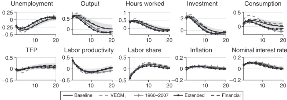
Figure 2 compares the IRFs of the shock that targets the business-cycle volatility of the unemployment rate (black line) to the IRFs of the shocks that are identified by targeting the business-cycle volatility of some other key macroeconomic quantities: GDP, hours, investment, and consumption.
As is evident from the figure, these shocks are nearly indistinguishable: tar-geting any one of the aforementioned variables seems to give rise to the same dynamic comovement properties. This explains the rationale of interpreting these reduced-form shocks as interchangeable facets of the empirical footprint of the same propagation mechanism, or of what we have called the MBC shock.12 Online
12 Recall that, for our purposes, different shocks that are observationally equivalent in terms of IRFs are
essen-tially one and the same shock. This perspective is consistent with standard practice in both the SVAR and the DSGE literatures: as echoed in the quote from Cochrane cited in footnote 2, shocks are visible, and hence distinguishable, only through the dynamic comovement patterns they induce in the variables of interest.
Appendix G.7 reinforces this rationale by including in our VAR two familiar gap measures, the gap between actual and potential GDP and the gap between actual unemployment and NAIRU, and by showing that the shock that targets either gap is also indistinguishable from the shocks seen in Figure 2.
Table 2 and online Appendix Table 28 paint a complementary picture in terms of the variance contributions: the shock that targets any one of unemployment, GDP, the corresponding gaps, hours, and investment explains the bulk of the business-cycle volatility in all of these variables. The following caveat applies to consumption: the shock that targets consumption explains less than one-quarter of the fluctuations in unemployment, hours, or investment; and symmetrically, the other shocks that make up our MBC template account for less than one-quarter of the fluctuations in con-sumption.13 Nonetheless, the consumption shock is very similar to the other shocks
with regard to both the IRFs and the disconnect from TFP and inflation. That is, it shares roughly the same propagation mechanism.
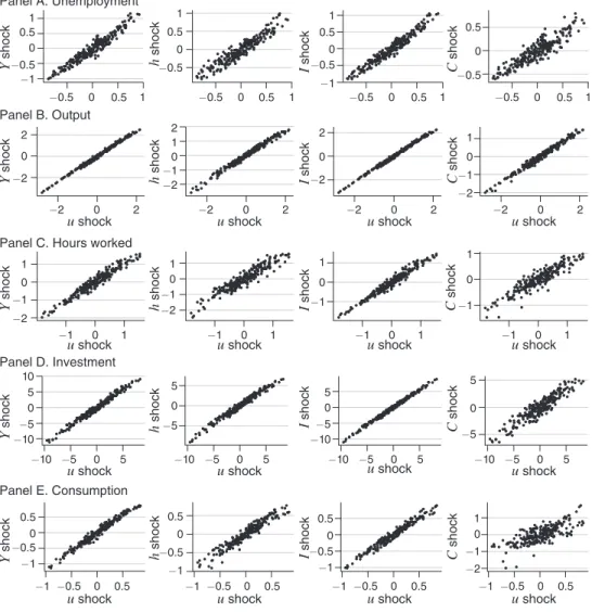
Finally, the interchangeability property extends from the IRFs to the time series produced by the different versions of the MBC shock. This is shown in Table 3. The table reports, for any of the variables of interest, the correlations between the times series of that variable produced by the unemployment shock and that produced by any of its sister shocks. The nearly perfect correlations seen in this table mean that recovered shocks are essentially the same, not only in terms of IRFs, but also in terms of realizations, as manifested in the times series they produce for the main variables of interest.14
13 Recall that consumption excludes spending on durables, which is instead included in investment. 14 Let X ∈ {u, Y, C, I, h} denote any one of the variables of interest. Next, let X
s denote the bandpass-filtered
time series of the predicted value of that variable produced by the shock that targets the variable s ∈ {u, Y, C, I, h} (where s may or may not coincide with X ). We are using the band pass filter suggested by Christiano and Fitzgerald (2003). The typical cell in Table 3 reports, for a variable X (across rows) and a shock s ≠ u (across columns), the correlation of X s and X u . This summarizes the information seen in Appendix Figure B1, which depicts the full
scat-terplots of the series X s against the series X u , for all X and s . The similarity is also present in terms of the innovations
that correspond to the different shocks. For instance, the correlation between the ε identified by targeting unemploy-ment and that identified by targeting output is 0.86. But these innovations, and the corresponding column vectors
Figure 2. The Various Facets of the MBC Shock, IRFs
Note: Shaded area: 68 percent HPDI.
10 20 Unemployment 10 20 Output 10 20 Hours worked 10 20 Investment 10 20 10 20 0.25 0.5 −0.5 −0.25 −0.5 0 0 0.5 −0.5 0 0.5 −0.5 0 0.1 −0.1 0 0.1 −0.1 0 0 0.5 1 0 0 0 2 0.5 0.5 1 10 20 10 20 10 20 10 20 Consumption
TFP Labor productivity Labor share Inflation Nominal interest rate
C. The Long Run and the Short Run
In the preceding analysis we recovered a MBC shock by targeting the business cycle frequencies. We now document the existence of an analogous object for the long-run frequencies. We also discuss the implications of our results for theories that link the business cycle to technology and news shocks.
Consider the shocks that target GDP, investment, consumption, TFP, and labor productivity at the frequencies corresponding to 80– ∞ quarters. Figure 3 and Table 4 show that these shocks are nearly indistinguishable in terms of IRFs and variance
of the matrix Q , are not sufficiently meaningful in their own right. What matters is how these innovations propagate over time and across variables, which is what the IRFs seen in Figure 2 reveal, or how they manifest themselves in terms of the predicted time series X s , which explains the focus of Table 3 and Figure 9.
Table 2—The Various Facets of the MBC Shock, Variance Contributions
Targeted variable: u Y h I C Unemployment 73.7 57.8 46.9 61.1 20.0 [66.7, 79.8] [50.5, 65.1] [39.6, 53.9] [54.7, 67.9] [13.7,27.0] Output 55.6 79.8 44.0 66.5 32.6 [49.6, 61.7] [72.9, 86.2] [36.7,51.3] [61.0, 72.6] [26.0,39.2] Hours worked 49.0 46.5 70.0 46.7 21.7 [41.8, 56.3] [38.0, 55.3] [63.0, 76.7] [37.3, 55.6] [15.6,28.5] Investment 58.2 66.2 44.4 80.1 18.8 [52.3, 64.0] [60.2, 72.3] [36.8, 51.9] [73.5, 86.6] [12.5,26.3] Consumption 18.3 30.9 19.5 16.2 67.8 [12.2, 25.8] [22.5, 39.3] [13.4, 26.1] [10.2, 24.1] [60.7, 75.3] Targeted variable: TFP Y / h wh / Y π R Unemployment 5.7 23.6 26.9 6.8 21.8 [2.6, 10.8] [17.2, 31.0] [18.5, 35.6] [3.3, 12.0] [14.6, 30.9] Output 4.1 41.0 40.5 10.6 16.8 [1.7, 8.4] [35.3, 47.2] [33.7, 46.8] [6.1, 16.1] [10.3, 25.0] Hours worked 11.5 22.0 19.4 7.0 22.4 [6.4, 18.2] [15.4, 29.4] [11.1, 29.5] [3.5, 12.5] [14.6, 31.5] Investment 3.7 33.9 36.5 7.4 20.6 [1.3, 7.9] [27.7, 40.2] [29.5, 43.4] [3.6, 12.5] [13.3, 29.1] Consumption 1.5 12.6 9.8 9.5 4.5 [0.6, 3.4] [7.4, 18.4] [5.0, 16.9] [4.6, 16.9] [1.3, 10.3]
Notes: The rows correspond to different targets in the construction of the shock. The columns give the contributions of the constructed shock to the business-cycle volatility of the variables. 68 percent HPDI in brackets.
Table 3—Correlations of Conditional Times Series
Y shock I shock C shock h shock
Unemployment 0.971 0.981 0.923 0.939
Output 0.997 0.997 0.989 0.992
Investment 0.990 0.996 0.934 0.989
Consumption 0.986 0.982 0.744 0.961
Hours worked 0.971 0.981 0.923 0.939
Note: Each row reports the correlation between each bandpass-filtered variable as predicted by the unemployment shock and that predicted by the other facets of the MBC shock.
contributions. Hence, one may advance the concept of the “main long-run shock” in a manner analogous to that of the MBC.15
This finding also motivates us to repeat our exercises using a VECM in which the aforementioned quantities share a common stochastic trend, while the remaining variables are stationary. The use of such a VECM instead of our baseline VAR is recommended if the analyst has a strong prior that the aforementioned quantities are cointegrated: a prior that is not only imposed in standard models but also corrobo-rated by the evidence presented above as well as by familiar co-integration tests. For robustness, we also consider a variant VECM in which we add a second stochastic trend that drives inflation and the nominal interest rate. This helps capture the famil-iar indeterminacy of the long-run values of these variables in theoretical models and their high persistence in the actual data.
15 We have verified that the shocks considered here are nearly identical to those identified by targeting the
fre-quency exactly at ∞ , which amounts to imposing a set of long-run restrictions as in Blanchard and Quah (1989) and Galí (1999). A similar picture also emerges from inspection of the first principal component over these long term data; see online Appendix Table 18.
Figure 3. Long-Run Shocks
Note: Shaded area: 68 percent HPDI.
10 0 0 0 0.5 0.5 1 0 0.5 −0.5 1 0 0 0.5 −0.5 0 0.2 −0.2 0 0.2 −0.2 0 0.5 1 3 2 1 0 −0.2 20 Unemployment 10 20 Output 10 20 Hours worked 10 20 Investment 10 20 10 20 10 20 10 20 10 20 10 20 Consumption
TFP Labor productivity Labor share Inflation Nominal interest rate
Yshock Ishock Cshock Y/hshock TFP shock
0.5
Table 4—Long-Run Shocks, Contributions at Long-Run Frequencies (80-– ∞ Q)
Targeted variable: Y I C TFP Y / h Output 99.7 96.7 99.6 96.3 97.2 [98.7, 99.9] [90.1, 99.0] [98.6, 99.9] [89.4, 98.9] [91.9, 99.2] Investment 97.4 98.2 97.0 92.3 92.8 [90.2, 99.4] [94.8, 99.5] [89.6, 99.3] [77.2, 97.9] [76.4, 98.0] Consumption 99.5 96.4 99.6 96.0 97.0 [98.2, 99.9] [89.3, 98.9] [98.6, 99.9] [88.9, 98.9] [91.4, 99.2] TFP 97.6 93.7 97.6 98.7 98.6 [90.3, 99.4] [79.5, 98.2] [90.4, 99.5] [95.5, 99.7] [95.6, 99.7] Labor productivity 98.5 94.2 98.7 98.0 99.1 [93.5, 99.6] [81.4, 98.4] [94.1, 99.7] [92.8, 99.5] [95.8, 99.8]
These VECMs produce the same empirical properties for the MBC shock as those derived from the VARs and presented above. They also produce similar pat-terns regarding the properties of the long-run shock. Table 5 demonstrates this with regard to the business cycle footprint of the long-run shock. This table reports the contribution of the main long-run shock, represented by the shock that targets TFP over the 80– ∞ range, to the volatilities of all the variables over the 6–32 range. The emerging picture is essentially the mirror image of that contained in the second row of Table 1. There, we reported that the MBC shock has a small contribution to the long run. Here, we see that the shock that accounts for the long run has a small footprint on the business cycle.
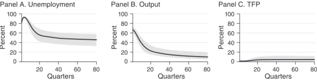
The disconnect between the short and the long run can also be seen in Figure 4, which shows the contribution of the MBC shock to the forecast error variance (FEV) of unemployment, output, and TFP at different time horizons.16 The MBC shock
explains more than 60 percent of unemployment and output movements during the first two years, but less than 7 percent of the TFP movements at any horizon; and conversely, the main long-run shock explains nearly all the long-run variation in investment and TFP, but less than 10 percent of the unemployment and investment movements over the first two years.17
How do these findings compare to related ones in the existing literature?
First, consider Blanchard and Quah (1989). This paper seeks to represent the data in terms of two shocks, a “supply shock” and a “demand shock.” To this goal, they run a VAR on two variables, GDP and unemployment; identify the supply shock as the shock that accounts for GDP movements in the very long run (at ∞ ) and the demand shock as the residual shock; and document that the supply shock accounts for about 50 percent of the business-cycle volatility in GDP and a bit more of that in unemployment. The additional information contained in our larger VAR reduces the contribution of the supply shock to about 12 percent for GDP and for unemployment.
16 The MBC shock is still identified in the frequency domain. The same picture emerges when the MBC is
identified in the time domain, provided that one uses the “right” mapping between the two domains. See online Appendix Section E.
17 It is worth noting that the disconnect between the short and the long run extends from neutral technology,
as measured by TFP, to investment-specific technology, as measured by the relative price of investment; see online Appendix Section G.2.
Table 5—Long-Run TFP Shock, Contributions at Business-Cycle Frequencies
u Y h I C VAR 9.7 25.7 11.5 18.6 15.7 [3.9, 18.9] [11.7, 42.5] [5.1, 20.1] [8.2, 31.3] [6.7, 27.9] VECM 12.1 11.7 8.0 10.6 8.6 [4.8, 22.1] [4.7, 22.4] [2.8, 16.3] [4.5, 19.3] [2.3, 18.5] TFP Y / h wh / Y π R VAR 21.4 22.9 10.2 13.1 8.1 [6.6, 41.8] [11.4, 36.4] [2.8, 23.2] [4.9, 27.8] [2.8, 16.9] VECM 11.5 11.2 9.5 7.7 11.1 [3.8, 26.6] [5.0, 22.4] [4.2, 18.6] [2.4, 21.1] [3.5, 25.2]
Second, consider Uhlig (2003), which is the closest predecessor to our paper. Similarly to Blanchard and Quah (1989), Uhlig (2003) pursues a two-shock rep-resentation of the data. The two shocks are identified by jointly maximizing the forecast error variance (FEV) in real GNP for horizons between 0 and 5 years. Uhlig offers a tentative interpretation of one shock as being a productivity shock of the RBC type and the other as a cost-push shock of the New Keynesian type. This interpretation finds little support in our more extensive anatomy of the data, especially due to our finding of a disconnect between our MBC shock and TFP at all horizons.18 Furthermore, as explained in Section IIIB, once we move from the
frequency to the time domain, the business cycle is best captured by targeting the FEVs of unemployment and GDP at 1 year, as opposed to longer horizons.
Third, consider Galí (1999) and Neville et al. (2014). Our long-run TFP shock is essentially the same as the technology shock identified in those papers. Tables 4 and 5 confirm their finding that this shock has a small contribution to the business cycle. This extends to the robustness exercises reviewed in Section IIIC.
Finally, consider Beaudry and Portier (2006). The first part of that paper uses a two-variable VAR with TFP and the S&P500 index to identify a shock that has zero impact effect on TFP but accounts for the bulk of both the short-run movements in stock prices and the long-run movements in TFP. This shock is interpreted as “news” about future TFP. The second part proceeds to argue, using 3–5-variable VARs and additional identifying restrictions, that TFP news shocks account for about 50 per-cent of the short-run volatility in hours and total private spending, about 80 perper-cent of that in consumption, and about 80 percent the long-run movements in private spending. In short, TFP news emerges as the main driver of both the business cycle and the long run.
This picture is hard to reconcile with our results, as well as with those of Galí (1999) and Neville et al. (2014). If TFP news was the main driver of both the busi-ness cycle and the long run, one would expect to see a strong connection between the two. But as seen in Table 5, the main long-run shock identified here accounts for only 10 percent of the short-run volatility in unemployment, hours, and investment. A similar disconnect is found in Galí (1999) and Neville et al. (2014).
18 We emphasize that the interpretation offered in Uhlig (2003) was tentative as that paper was not completed.
Also note that the approach adopted in that paper allows for the identification of the two shocks together but does not separate one shock from the other, so the aforementioned interpretation relied on particular orthogonalizations. Finally, because the VAR considered in that paper did not contain TFP, the disconnect documented here could not have been detected.
Figure 4. FEVs of Unemployment, GDP, and TFP to the MBC Shock
Note: Shaded area: 68 percent HPDI.
20 40 60 80 Quarters Percent Panel A. Unemployment 20 40 60 80 Quarters Percent Panel B. Output 20 40 60 80 Quarters 0 20 40 60 80 100 Percent Panel C. TFP 0 20 40 60 80 100 0 20 40 60 80 100
Perhaps most tellingly, Figure 4 shows that the MBC shock accounts for nearly zero of the FEV of TFP at any horizon. That is, the MBC shock itself contains no news about future TFP.19
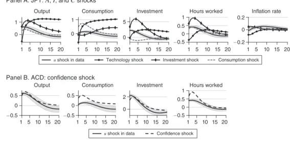
We believe that, while TFP news may be a nontrivial contributor to macroeco-nomic fluctuations, the numbers reported by Beaudry and Portier (2006) exaggerate its importance due to the use of smaller VARs and different identifying assumptions. We elaborate on these points in Section IV and Appendix Section C. There, we use a semistructural exercise, based on our anatomy of the data, to shed new light on the business-cycle effects of technology and news shocks. Our explorations suggest that the contribution of news shocks to unemployment fluctuations is about 10 percent, which is much more modest than that suggested by Beaudry and Portier (2006) and closer to that reported in Barsky and Sims (2011).
A similar challenge applies to Lorenzoni (2009). That paper emphasizes the role of noise in the signals of future TFP, but maintains the core hypothesis that the busi-ness cycle is driven by shifts in the rational expectations of the long run, which is hard to reconcile with our findings.20
What is left open is the possibility that the identified MBC shock reflects either
irrational beliefs about the long run, or news about the short run. A formalization of the latter kind of news is found in our companion paper (Angeletos, Collard, and Dellas 2018), to which we return in Section V.
D. Inflation and the Business Cycle
We now turn attention to the nexus of real economic activity and inflation. Our method identifies a weak link. First, as shown in the first row of Table 6 (which repeats a portion of the first row of Table 1), the identified MBC shock accounts for only 7 percent of the business-cycle variation in inflation, which is as low as the corre-sponding number for TFP. Second, the shock that targets inflation explains 83 percent of the business-cycle volatility in inflation and only 4 to 8 percent of that in unem-ployment, output, and investment. Third, the shock that targets inflation explains only 2 percent of the labor share, a proxy of the real marginal cost or the “fundamental” in the New Keynesian Phillips Curve (Galí and Gertler 1999); and symmetrically, the shock that targets the labor share explains 86 percent of the labor share itself but only 4 percent of inflation. Fourth, the shock that targets inflation is essentially orthogonal to the MBC shock, both in terms of innovations and in terms of induced series. For instance, the correlation between the ε identified by targeting inflation and that iden-tified by targeting unemployment is 0.047. Finally, online Appendix Sections G.6 and G.7 show that these findings are robust to different measures of inflation (GDP deflator versus CPI, PPI, or core inflation) and different measures of real slackness (unemployment versus unemployment gap or output gap).
What is the lesson for theory? Because of its transitory nature and its disconnect from TFP, it is tempting to interpret the MBC shock in the data as a demand shock in the New Keynesian model. However, in that model demand shocks generate
19 As verified in row 9 of Table 8, these findings are robust to the inclusion of Stock Prices in the VAR. 20 By shifting the focus from the distinct theoretical formulation of news and noise shocks to their shared empir-ical footprint in terms of VAR representations, we echo Chahrour and Jurado (2018).
business cycles only by inducing positive output gaps from flexible-price outcomes. Furthermore, because replicating flexible-price outcomes is equivalent to stabiliz-ing inflation, such gaps are the main “fundamental” drivstabiliz-ing inflation. In particular, insofar as business cycles are predominantly demand-driven and the Phillips curve is not exceedingly flat, the New Keynesian model imposes that inflation is the best predictor of future output gaps, or real marginal costs, similarly to how the basic asset-pricing model imposes that asset prices are the best predictor of future earn-ings. From this perspective, Table 6 suggests that the failure of the two models is comparable: the link between inflation and real economic activity is no stronger than the link between asset prices and earnings.21
Another challenge emerges from contrasting the magnitude of the actual inflation response to the identified MBC shock to that predicted by the calibrated, textbook version of the New Keynesian model under the interpretation of this shock as an aggregate demand shock: as illustrated in online Appendix Figure 25, the predicted response is over ten times larger than the observed one.
These challenges are familiar, albeit through other metrics.22 The DSGE
liter-ature has sought to address them by making the Phillips curve much flatter than, not only its textbook version, but also that implied by menu-cost models calibrated to microeconomic evidence; and by attributing almost the entirety of the observed inflation fluctuations to large markup shocks or some other “residual.”
The empirical foundations of these and other features that help improve the empir-ical fit of DSGE models remain a contested issue. Needless to say, this does not mean that we question the empirical relevance of nominal rigidities, or the nonneutrality of monetary policy. But we do wish to raise the possibility that the MBC shock in the data represents an aggregate demand shock of a different kind than that presently formalized in the New Keynesian framework, namely one that operates inside its flexible-price core rather than outside it. This echoes the common message of Angeletos and La’O (2013), Beaudry and Portier (2014), and the literature cited in footnote 3.
Finally, consider the argument made in McLeay and Tenreyro (2020) that the dis-appearance of the empirical Phillips curve in the post-Volker era (i.e., the absence of a
21 As one would expect, the link improves somewhat if we focus on the pre-Volker period. See row 7 of Table 8. 22 For instance, the weak comovement of inflation and real economic activity is also evident in the
uncondi-tional moments, although it is less pronounced than that seen in Table 6. See also Atkeson and Ohanian (2001); Mavroeidis, Plagborg-Møller, and Stock (2014); Stock and Watson (2007, 2009); and Dotsey, Fujita, and Stark (2018) for examples of works that document a similar statistical disconnect between gaps and inflation as that documented here, albeit with different methods. And finally see the survey by Mavroeidis, Plagborg-Møller, and Stock (2014) and the references therein for empirical performance of the various incarnations of the Phillips curve.
Table 6—Inflation and the Business Cycle
Targeted variable: u Y π wh/Y Unemployment 73.7 57.8 6.8 26.9 [66.7, 79.8] [50.5, 65.1] [3.3, 12.0] [18.5, 35.6] Inflation 4.2 8.0 83.3 1.9 [1.8, 8.6] [4.0, 13.1] [76.2, 88.3] [0.7, 4.4] Labor share 26.0 35.6 4.0 85.4 [18.7, 33.5] [28.8, 42.6] [1.7, 7.6] [79.8, 90.4]
strong positive relation between inflation and the output gap) may reflect a monetary policy that has done a good job in stabilizing the output gap against demand shocks and has let inflation be driven primarily by “residual” shocks. This argument may explain the disconnect seen in Table 6 in terms of variance contributions. But another key piece of evidence produced by our anatomy is the muted response of inflation to the MBC shock (seen earlier in Figures 1 and 2). This in turn requires either that the structural Phillips curve is exceedingly flat,23 which runs against the thesis of the
aforementioned paper, or that the MBC shock is a demand shock that generates real-istic business cycles even when monetary policy replicates flexible-price allocations, which circles back to our preferred interpretation of the evidence.
III. Robustness
In this section we first discuss the relation between our approach and two alterna-tives: principal component analysis, and identification in the time domain. We next report results from an extensive battery of robustness exercises conducted.
A. The MBC Shock and Principal Component Analysis
The finding that there is a single force that drives multiple measures of economic activity naturally invites a comparison to principal component analysis (PCA). Is our MBC shock similar to the first principal component of the data over business-cy-cle frequencies? And if yes, are there any reasons to favor employing our method over PCA in pursuing an anatomy of the business cycle?24
To address the first question, we perform PCA in the frequency domain. For each variable X j ∈
{
u, Y, h, I, …}
, we construct the bandpass-filtered variable X jbcthat isolates its business cycle frequencies ( 6–32 quarters). We then use the cova-riance matrix of all the filtered variables to construct the first principal component, denoted by PC 1 bc . We finally project each X
j
bc on PC 1 bc and compute the R2 of the
projection. This gives the percentage of the business-cycle volatility in variable j accounted for by the principal component.25
Four different versions of this exercise are carried out. In the first version, X bc is
derived by applying the bandpass filter directly on the raw data, variable by vari-able. In the second version, we first run a VAR on all the variables jointly, use it to estimate the cross-spectrum of the data, and then construct the band passed vari-ables X jbc . Hence, the bandpass filter is the ideal one in the latter case, whereas it is
only an approximate one in the former.
In the third and fourth version, the filtered variables are normalized by their respective standard deviations before extracting the first principal component. Such a normalization is often employed in the PCA literature in order to cope with scaling
23 See online Appendix Section I.1 for the illustration of this point when the MBC shock maps directly to a
demand shock in the New Keynesian model; and see online Appendix Section I.2 for the robustness of this point to letting the MBC shock map to a mixture of demand and supply shocks in the model.
24 We thank an anonymous referee for suggesting the exploration of these questions.
25 Recall that the first principal component is constructed by taking the eigenvector corresponding to the largest
eigenvalue of the covariance matrix. It is thus designed to account for as much as possible of the volatility and the comovement of all the (filtered) variables at once.
issues and/or to focus on the comovements in the data. But it also reduces the role played by the more volatile variables (e.g., investment), which may or may not be desirable depending on the context. As we do not have a strong prior on how to properly weight the variables, we carry the exercise on both normalized and nonnormalized data.
The results are reported in Table 7. In all cases, the first principal component accounts for the bulk of the business-cycle volatility in unemployment, hours, out-put, and investment but for only a small fraction of the business-cycle volatility in either TFP or inflation.
This is reassuring: the picture obtained here is similar to that obtained in Table 2 about the various facets of the MBC shock. As shown in online Appendix Section F, a similarly reassuring connection holds between the main long-run shock obtained by our method in the next section and the principal component obtained by applying PCA to the long-run components of the data.
However, there are three key pieces of information that our approach produces but PCA does not. First, PCA is not useful for addressing the question of whether the forces that drive the business cycle and long run are related, because the afore-mentioned two principal components are orthogonal to each other by construction. Second, PCA does not contain information about how the variables respond on impact and over time to a shock; that is, PCA does not accommodate the construc-tion of IRFs, which are of paramount importance for our purposes. And third, by targeting individual variables, our method avoids the difficulties associated with having to choose the “best” weights in PCA and, more importantly, helps reveal patterns that prove useful in the validation of existing models or in the construction of new ones.
A version of Dynamic Factor Analysis, appropriately adapted to the frequency domain, could address the first two caveats and offer a useful complement to our approach. But it would not immediately accommodate the third point: the informa-tion extracted by taking multiple cuts of the data.
B. MBC in the Frequency Domain versus the Time Domain
A long-rooted convention in empirical macroeconomics identifies the business cycle with the fluctuations occurring in the 6–32 quarters range in the frequency
Table 7—The First Principal Component, Business-Cycle Frequencies
u Y h I C Raw data 75.3 92.3 81.2 99.8 60.2 VAR-based 60.5 86.0 58.2 99.7 23.7 Normalized data 91.5 86.8 91.3 80.6 76.7 VAR normalized 80.8 90.0 77.0 80.7 50.4 TFP Y / h wh / Y π R Raw data 6.1 17.7 3.0 2.3 12.3 VAR-based 0.6 22.8 11.6 2.5 12.8 Normalized data 17.3 2.6 0.3 19.2 38.2 VAR normalized 1.8 9.7 3.5 7.1 29.8
domain (FD).26 In line with this tradition, our MBC shock is constructed by
identi-fying the shock that accounts the most of the volatility of unemployment and other key macro quantities in that range.
But suppose one wished to identify business cycles in the time domain (TD) instead. Which horizon(s) should one target?
At first glance, one may think that targeting volatility over the 6–32 quarters band in the FD is equivalent to targeting volatility over the 6–32 quarters horizon range in the TD. But this is wrong: such a relation does not hold for arbitrary DGPs (or arbitrary models), nor does it hold in the actual data.
We offer a comprehensive treatment of this issue in Appendix Section E by under-taking two exercises, one theoretical and one empirical.
In the first exercise, we set up a 3 × 3 model (three variables, three shocks). Although the model is deliberately abstract, its variables can loosely be interpreted as unemployment, output, and inflation. Its main purpose is to serve as a controlled laboratory environment, in which we can work out the properties of alternative map-pings between the FD and the TD.
Within this controlled environment, we establish two properties of the MBC shock identified via our method, that is, by targeting the volatility of the first two variables over the 6–32 quarters in the FD: (i) this shock is notably different from the shock that targets 6–32 quarters in the TD; and (ii) this shock is nearly identical to the one that targets 4 quarters in the TD. This serves both as a proof of concept that the mapping between the FD and the TD is nontrivial in general, and as an illus-tration of the kind of model that best fits the data.
The second exercise completes the picture by showing that the two properties mentioned above indeed characterize the data. A hint that the second property is true in the data was already present in Figures 1 and 4, which showed that the footprint of our MBC shock in the TD, in terms of both IRFs and FEVs, peaked within a year or so.
These findings complement the picture painted in the rest of our paper. They also illustrate why TD-based identification strategies that maximize the FEV contribu-tion of a shock to unemployment or output at longer horizons could fail to capture business cycles.
C. Alternative Specifications
We now turn to the robustness of our main results along various dimensions (sample periods, set of variables, assumptions about stationarity, numbers of lags). The main exercises are described below; a few additional ones are relegated to the online Appendix.
Table 8 describes the variance contribution of the MBC shock over business-cy-cle and longer-term frequencies, respectively, and across many alternative specifi-cations (different samples, statistical models estimated, set of variables, numbers of lags). As in Table 1, we use the shock that targets unemployment as the measure of
26 This convention stretches back at least to Mitchell. More recently, when researchers document business-cycle
moments whether in the data or in a model, they almost invariably use either the BP filter at the 6–32 quarters band or the HP filter, which is closely related (e.g., Stock and Watson 1999).