Publisher’s version / Version de l'éditeur:
Vous avez des questions? Nous pouvons vous aider. Pour communiquer directement avec un auteur, consultez la première page de la revue dans laquelle son article a été publié afin de trouver ses coordonnées. Si vous n’arrivez pas à les repérer, communiquez avec nous à [email protected].
Questions? Contact the NRC Publications Archive team at
[email protected]. If you wish to email the authors directly, please see the first page of the publication for their contact information.
https://publications-cnrc.canada.ca/fra/droits
L’accès à ce site Web et l’utilisation de son contenu sont assujettis aux conditions présentées dans le site LISEZ CES CONDITIONS ATTENTIVEMENT AVANT D’UTILISER CE SITE WEB.
The 17th International Workshop on Qualitative Reasoning [Proceedings], 2003
READ THESE TERMS AND CONDITIONS CAREFULLY BEFORE USING THIS WEBSITE. https://nrc-publications.canada.ca/eng/copyright
NRC Publications Archive Record / Notice des Archives des publications du CNRC :
https://nrc-publications.canada.ca/eng/view/object/?id=98db93a9-0ad7-4a70-a49d-e2dbe13ef77c
https://publications-cnrc.canada.ca/fra/voir/objet/?id=98db93a9-0ad7-4a70-a49d-e2dbe13ef77c
NRC Publications Archive
Archives des publications du CNRC
This publication could be one of several versions: author’s original, accepted manuscript or the publisher’s version. / La version de cette publication peut être l’une des suivantes : la version prépublication de l’auteur, la version acceptée du manuscrit ou la version de l’éditeur.
Access and use of this website and the material on it are subject to the Terms and Conditions set forth at
Qualitative Model Abstraction for Diagnosis
National Research Council Canada Institute for Information Technology Conseil national de recherches Canada Institut de technologie de l'information
Qualitative Model Abstraction for Diagnosis *
Yan, Y.
August 2003
* published in The 17th International Workshop on Qualitative Reasoning. Brasilla, Brazil. August 20-22, 2003. pp. 171-179. NRC 46498.
Copyright 2003 by
National Research Council of Canada
Permission is granted to quote short excerpts and to reproduce figures and tables from this report, provided that the source of such material is fully acknowledged.
Qualitative Model Abstraction for Diagnosis
Yuhong Yan
NRC Institute of Information Technology, Canada [email protected]
Abstract
Building qualitative models is a crucial task for model-based diagnosis. This paper discusses the techniques to automatically transform a quantitative model in CAD environment into a qualitative model, under the cases that the real numbered landmarks are known and unknown. With known landmarks, the abstraction is through the discretization process where the simulation data is discretized according to the given landmarks. If landmarks are unknown, the landmark generation process, which is inspired by the discriminability analysis for multiple behaviour modes, is applicable. For dynamic systems, the pseudo-variables are introduced to describe the dynamic behaviour. The techniques developed are demonstrated by a simplified automotive subsystem.
Introduction
The automobile industry has foreseen the growing demand of diagnostic analysis for automobiles. Engineers need an integrated design environment that enables them to do the diagnostic analysis at the design stage, so that they can understand and evaluate the effects of each choice on the diagnostic properties of the system being designed. European FP5 Project IDD (Integrated Design Process for On-board Diagnosis) aims to formalize and standardize the diagnostic design process and to develop new techniques and tools to support this purpose. After a model-based diagnosis approach is determined, the problem of creating the appropriate qualitative model becomes the crucial issue. Our starting point is the numeric simulation model which is built to examine a system’s behaviour by design engineers in a CAD environment. Matlab/Simulink is the target CAD platform due to its wide adoption in the automotive industry. Models in Matlab/Simulink are illustrated graphically as a set of subsystems/blocks and a number of interconnected input and output links between the blocks. Empirical data, library functions, as well as formulas can be used in the blocks. Normally no explicit equations are available for the general system under study. Our task is to develop automatic approaches to abstract the qualitative model for diagnostic purposes.
The qualitative model used in this paper is in finite domain tuples, i.e. the domain of a variable has multiple landmarks. This paper presents the techniques of model abstraction with or without landmarks for both static and dynamic systems. Section 2 reviews the relevant techniques
for model abstraction and diagnosis. Section 3 discusses the approaches for model abstraction with known landmarks for both static and dynamic system. Section 4 represents the approach for the landmark determination based on diagnosability analysis. Section 5 demonstrates how the approaches developed can be used in a model of a subsystem in automotive. Section 6 is discussion and conclusion.
State of the Art in Qualitative Model
Abstraction and Diagnosis
State-based vs. Simulation-based Diagnosis
Diagnosing dynamic system requires checking the consistency of observations over time with the behaviours modeled by the dynamic model of the device. A straightforward solution is to simulate incrementally the model as observations change, in order to predict the immediate successor states. This is the simulation-based approach used in (Dvorak and Kuipers 1992). (Dressler 1996) avoids simulation and generates diagnostic candidates based on checking consistency of the model with observed states only. (Malik and Struss 1996) states a necessary and sufficient condition for the equivalence of state-based and simulation-based diagnosis without giving a proof. (Struss 1997) further presents that if the system dynamic can be modeled as state constraints plus CID constraints, which are general rules about continuity, integration and derivatives, then diagnosis based on checking the state consistency yields results equivalent to diagnosis based on simulation. Of course, the state-based approach is much less costly than the simulation-based approach. If a system has other temporal constraints than the CID constraints (called trans-constraints), the conclusion is no longer held. These trans-constraints are typically constraints introducing discontinuities over time. (Panati and Dupre 2000) and (Dupre and Panati 1998) report a violating case where abrupt faults are considered. Abrupt faults, where a system parameter changes abruptly, are the cases of discontinuity. By adding constraints related to injecting a fault, the simulation may actually be useful to restrict the set of possible diagnoses. There are many methods on how to model the constraints related to injecting a fault (Dupre and Panati 1998), (Mosterman and
Biswas, 1997). Abrupt faults are not considered in this paper.
The state-based diagnosis engine is used in our project, though the state-based way could result in more candidates as stated above. This paper concerns building a qualitative model efficiently and automatically from the simulation environment for the state-based diagnosis engine. Diagnosis equivalence in (Struss, 1997) has a precondition that there are sufficient observables. More specifically, since the state-based approach does not use the relation between x and dx/dt, both x and dx/dt should be observables in order to have enough redundancy for diagnostic analysis. Sometimes not both of x and dx/dt are modeled in the simulation model or not both can be measured as physical variables. In section 3.3, pseudo variables are introduced to describe the dynamic behaviour and also provide redundancy for diagnostic analysis for dynamic system.
Abstraction of Qualitative model
Qualitative models have already been successfully used in the framework of model-based diagnosis. When abstracting a qualitative model for a system, the crucial requirement is to transform the model to the right level of abstraction after composing it. In (Struss 2002), the problem is stated as to find the necessary and sufficient distinctions in the domains of the system variable to achieve a particular goal in a certain context and under given conditions. The right level of abstraction is task-dependent; depending on the requirements of the tasks, the distinctions can be different. (Sachenbacher and Struss 2001) introduces AQUA, a framework for automated qualitative abstraction. In AQUA, the goal of using a model is characterized by a set of target partitions of the domains of selected variables (e.g. output variables), the context is given by the structure of the model system, and the conditions are represented by a set of initial variables and their possible distinctions (e.g. possible observations). AQUA needs a fine-grained qualitative relation as the starting point. The partitions of domain can be given by (finite) sets of landmarks that define qualitative values as intervals between adjacent landmarks. AQUA then eliminates landmarks that do not contribute to a distinction between target partitions. The abstract model will then contain a subset of the landmarks of the original model but maintain the predictive power with respect to qualitative values of the target variables. One difficulty of this method is that the starting “fine” domain model is difficult to obtain. We do not know how fine the starting model should be, so that the abstract process can remove some landmarks to get the optimized qualitative model. Second there are no criteria to determine the target distinctions. (Struss 2002) extends AQUA by giving an approach to automatically determine the landmarks for the variables. It is a recursive subdivision process. The criterion to divide the domain is that if a qualitative value of some variable occurs in many tuples, it is identified as a candidate for refinement and split into two or more intervals by introducing additional
landmarks. This criterion does not show how the new partitions effect on the target distincts, thus its effectiveness is questionable.
Qualitative simulation is a widely used tool. The fundamental difference is QSIM starts from QDE (Qualitative Differential Equation) and the simulation is on qualitative level, while the starting point in this paper is the numerical simulation model, and the simulation is numerically. Many QSIM techniques, such as value generation, constraint filtering, can’t be used here. A summary of QSIM techniques and their extensions can be found in (Kuipers 2001).
In FDI community, there is also some work on building qualitative system models. One example is (Lunze et al. 1999), in which the state variables are partitioned along the time based the state transforms. The result is the discrete trajectory of states. In this paper, pseudo-variables, which are the derivatives of flow or effort variables (cf. section 3.3), are introduced to describe system dynamic. The pseudo-variables are equivalents to the state variables. While Lunze uses the state transform equations to determine the state variables in the next time step, our approach does not have transform equations. The discretization is on the values of input and output data after the time information is removed. Thus the two approaches are different from each other and both are suitable for their diagnosis principles.
There are some other commonly used ways to obtain qualitative model, e.g. the qualitative derivation model (Malik and Struss 1996), and Bond-graph analysis (Mosterman and Biswas 1997). They either have no automatic methods available or not start with simulation model. So they are not reviewed here. The techniques listed here are far from complete. A review on qualitative model construction can be found in (Schit and Bredeweg 1996).
Features of a Simulation Model and Its Gap to
Qualitative Model
There is a big gap between the simulation model which is a description of the system behaviours and the qualitative model which is used for diagnosis. The qualitative model for diagnosis needs two kinds of information: 1) the structural model which is the physical structure of a system, i.e. how the physical components are connected; 2) the behaviour model which is a description of the input-output relation for every physical component. In a graphical CAD environment, like Matlab/Simulink, the physical compo-nents are represented by blocks. A block can have sub-blocks for describing internal structure or functions inside the components. The links between the blocks are the physical connections, where the connected blocks have shared variables. The structural model is obtained by extracting the connections and block information from the CAD environment. This can be done by calling CAD functions to collect this kind of information. The difficulty is in abstracting the behaviour model. The relations of a
component are implied by the blocks. The standard blocks are normally mathematical operators and can be expressed as formulas between inputs and outputs. Many other so called “customized” blocks contain C-code, look-up tables and Matlab scripts, which have no explicit equations. These blocks can be cascaded or sub-composed together for one physical component. This gives the design engineers the maximum flexibility for building models. They can either encode their empirical data into the look-up tables, or embed logic clauses in the script code, or call professional libraries from C-code. But on the other side, this causes a great gap between a simulation model and a model-based diagnosis engine that requires explicit relational expression. Moreover, simulation is executed only in one direction, i.e. we are unable to compute the inputs from the outputs. Though the gap exists, one benefit of the CAD environment is its effective computation capacity to simulate the system behaviour in both static and dynamic processes. We can depend on this when we design our solution.
Abstracting Qualitative Models from
Simulation Models using Finite Domains
Finite Relation Qualitative Model
A Finite Relation Qualitative Model uses a set of real numbers as landmarks for each variable. The qualitative values are the intervals between adjacent landmarks. The qualitative relation is the mapping between the qualitative values. More landmarks produce a finer qualitative model.
Definition1: An interval is a pair of numeric landmarks: I1:=[lma, lmb], where lma ≤ lmb.
Definition2: Two intervals are equal if and only if the
two landmarks are equal:
For intervals I1:=[lma, lmb], and I2:=[lmc, lmd], I1 equals I2
iff lma= lmb and lmc= lmd.
Definition3: A tuple is a collection of ordered intervals: T:={I1, …, In} = {[lma, lmb],…, [lmp, lmq]}
If vectors LM1:= [lma,…, lmp] and LM2=[lmb,…, lmq], the
tuple T can be represented by T:=[LM1, LM2]. An
n-dimension tuple can represent an n-n-dimension rectangle.
Defintion4: A qualitative model q is a mapping
between two sets of intervals:
q: Ψ1→Ψ2. The source set Ψ1= {[lmiin, lmi+1in]} is the set of
qualitative inputs to the model, the target set Ψ2= {[lmkout, lmk+1out]} is the set of qualitative outputs from the model.
The mapping is a multiple valued relation, i.e. ∀ [lmi in , lmi+1 in ] ∈Ψ1 , q:[lmi in , lmi+1 in ]→Ψ2’ ⊂Ψ2 , Ψ2 is
empty or has one or more elements. If we can enumerate the mapping pairs, q can be presented in set of tuples, as: {{[lmiin, lmi+1in], [ lmjout, lmj+1out]},…{[lmpin, lmp+1in][ lmqout, lmq+1out]}} (1)
When the input is multi-demensional, a qualitative model
q is a mapping between two sets of tuples: q: ΨΨΨΨ1→ΨΨΨΨ2. The
source set ΨΨΨΨ1 = {Ti}is the set of input tuples and the target set ΨΨΨΨ2 = {Sj}is the set of output tuples of the model. If we
can enumerate the mapping pair of tuples, q can be represented by
{{T1, S1},{T2, S2},…,{Tn, Sm}} (2)
Definition5: If a system described by y=f(x) is a static
quantitative model, landmarks x1, x2,…,xn and y1, y2,…, ym
are selected for x and y and in an ordered sequence. A
qualitative abstraction q(f) is a mapping from set Ψ1 =
{[x1,x2],[x2,x3],...,[xn-1,xn]} to set Ψ2 ={[y1,y2],[y2,y3],...,[yn-1, yn]}:
q(f):{[x1,x2],[x2,x3],...,[xn-1,xn]}→{[y1,y2],[y2,y3],...,[yn-1,yn] },
such that:∀[xi,xi+1], q(f): [xi,xi+1]→[yj,yj+1], iff ∃x, xi≤x≤xi+1, yj ≤y≤ yj+1.
Qualitative abstraction q(f) results a qualitative model. Landmarks x1,x2,...,xn and y1,y2,...,ym are selected to cover y=f(x)’s domain and range, i.e. ∪i[xi, xi+1] ⊇ Domain(x),
and ∪j [yj, yj+1] ⊇ Range(y). Definition 5 can be extended
for multiple in-out systems.
Definition6: Y=f(X) is a static quantitative model,
where X= [x1, x2,…,xn] and Y=[y1, y2,…, ym]. [xi,1, xi,2,…,xi,n]
are landmarks for xi. [yi,1, yj,2,…, yj,m] are landmarks for yj.
A qualitative abstraction of model Y=f(X) is a mapping from set Ψ1= {Πi[xi,p, xi,p+1]} to set Ψ2= {Πj[yj,q, yj,q+1]}:
q(f): Ψ1→Ψ2, such that
∀
Πi[xi,p, xi,p+1], q(f): Πi[xi,p, xi,p+1]→Πj[yj,q, yj,q+1], iff ∃X,X∈Πi[xi,p, xi,p+1], Y∈Πj[yj,q, yj,q+1].
Model Abstraction for Static Simulation Model
with Known Landmarks
Discretization Algorithm is designed to deal with the
simplest case, in which the simulation model is static and the landmarks for the variables are known. The name come from that the algorithm discretizes the simulation data into intervals of landmarks.
Algorithm 1 is the discretization algorithm with the simulation model Y = f(X), where f can be implicit, and the landmarks for X and Y as inputs. Suppose xi has a set of
landmarks {x_lm1i , x_lm2i, …, x_lmmi}, the adjacent
landmarks makes a set of the intervals {[x_lm1 i
,x_lm2 i
],…, [x_lmm-1i, x_lmmi]}. The simulation inputs for xi are from
one of these intervals. Thus, the input points for X are generated from a multi-dimensional rectangle, which is one element in the set of the combination of the intervals: Πi{[x_lm1i,x_lm2i], …, [x_lmm-1i, x_lmmi]} , as in Line 2.
Suppose [x_lmpi, x_lmp+1i] is the interval for xi, k random
values are generated in this interval. For an n-dimensional rectangle, totally kn testing points generated (Line 3). The purpose of generating the random values is to probe the extrema when function f is not monotonic. This is just an approximate approach to deal with non-monotonic (ref. discussion below). Line 4 calls Simulink simulation function to get the values of the outputs for each of the kn testing points. Line5-6 gets the minimum and maximum output values. Line7-8 gets the landmarks that cover the range of output values. The qualitative relation is in line 9.
Algorithm 1: Discretization
Inputs:
Comp1 Comp2 E1 E2 E3 F1 F2 F3 Comp1 Comp2 E1 E2, dE2/dt F1 F2 F3 E3 dE3/dt
-{x_lm1i, x_lm2i, …, x_lmmi} is the set of landmaks for xi,
{y_lm1 j , y_lm2 j , …, y_lmq j
} is the set of landmarks for yj
- a nature number k Outputs:
- a vector q storing the mapping pair (as format in (2)) 1: create a vector q to store the mapping pair
2: for each element in Πi{[x_lm1i, x_lm2i], …, [x_lmm-1i, x_lmmi]}
3: generate k random values for each [x_lmp i
, x_lmp+1 i
], lets say {x_lmpi, xx1i,…, xxki, x_lmp+1i}, the input points are
Π{x_lmpi, xx1i,…, xxki, x_lmp+1i}
4: call Simulink function to simulate f(Πi{x_lmpi, xx1i, …, xxki, x_lmp+1i})
5: Ymin = min(f(Π{x_lmpi, xx1i,…, xxki, x_lmp+1i}))
6: Ymax = max(f(Π{x_lmpi, xx1i,…, xxki, x_lmp+1i}))
7: y_lowj = max({y_lmuj | y_lmuj yminj})
8: y_highj = min({y_lmvj | y_lmvj≥ ymaxj})
9: store <Π [x_lmm i , x_lmm+1 i ], [y_lowj, y_highj]> in q 10: end for 11: report q
Algorithm 1 is similar to the method in (Struss 2002). The similarities are both methods use real numbers as landmarks and discretize the continuous model with these landmarks. The differences are: first, (Struss 2002) considers the precision of the model, i.e. the base model is given by the envelope of f(X). This is perhaps for considering noise in the signals or the computation error in simulation. We consider it is not necessary to add this envelope. If concerning the noise, it is better to eliminate the noise from the signals than adding the tolerance at the modeling stage. If concerning about the computation error, it is rather small that ignoring it won’t affect the approximation of the qualitative model. Adding envelope could degrade the qualitative model because the distinctions between right and faulty behaviour might be removed. Secondly, (Struss 2002) limits the algorithm to monotonic functions or monotonic sections of a function. With the monotonic constraint, the tuples are determined by the bounding landmarks (e.g. the corners of the rectangle). If users do not know the shape of the function, users can choose wrong landmarks that the relation determined by the bounding landmarks can miss the extreme points, thus abstracted qualitative behaviour is not “sound”. To get the monotone pieces from the discrete simulation data is not a trivial problem. The way to compute the derivative numerically from the discrete simulation data in order to determine the monotone as in (Struss, 2002) is not feasible because the very small but numerous turbulences on the data, which is the case for the simulate data, could lead to wrong results. Our method using random points to probe the extrema between the landmarks is a practical solution for the non-monotonic function. If the random points are in a large amount, practically this method can get satisfactory results for non-monotonic systems. But this problem is still open. (Brooks, 1984) gives a mathematical foundation for detecting monotonic pieces from discrete data (simulation
data). We believe this could be a solution, though we did not test this technique yet.
Model Abstraction for Dynamic Model
As discussed in Section 2.1, there are two views on how to diagnose dynamic systems. State-based diagnosis is used in our project. In state-based diagnosis, the relations between the time steps are not considered, i.e. dx/dt is not computed from x, or when dx/dt and x are both known, the relation between them is ignored. One straightforward way to model the dynamic for state-based diagnosis is to model the derivatives of the variables. But in many situations, the derivative of a variable is not a variable in the simulation model, or physically is not a measurable variable. For example, Figure 1 is the model for a RC circuit. Voltages, u1, u2, and u3, are the observable variables, while current i is non-observable. u1 and u3 are constant. The derivatives of the voltages or the currents, which are necessary for modeling the dynamic behaviour, are missing in the simulation model.
Our solution is to introduce the pseudo variables, which are the derivatives of effort or flow variables, in the qualitative model. A systematic framework exists for building consistent and well constrained models of dynamic physical systems from multiple domains (e.g. electrical, mechanical, hydraulic), which is based on the
continuity of power and conservation of energy between
system components (Karnopp and Rosenberg 1975) The
effort variables are to represent generalized voltage,
pressure, temperature, etc., and the flow variables are to represent generalized current, volume flow, entropy flow, etc. Depending on the dynamic is caused by capacity or inertia element, the derivatives of effort or flow variables are chosen as the pseudo variables. As shown in figure 2, (a) is the original model, in which E is the effort vector, and F is the flow vector. For the system has capacity dynamic, dE/dt is added as pseudo variables, or for inertia dynamic, dF/dt is added as pseudo variable. Fig 2(b) is a case with capacity dynamic, in which dE1/dt to dE3/dt are added as pseudo variables. The pseudo variables are a part of the qualitative relations as the other variables.
For the RC example, the derivative of u2 (du2 in figure
R C u1 i i u2 u3 i R u1 C u2 u3
(a) RC Circuit (b) RC Circuit in block diagram Fig. 1 Example: RC Circuit and Simulation Model
(a) original model (b) model with pseudo variables Fig. 2 Dynamic System
R C u1 i i u2, du2 u3 i du2 i u2 i
3(a)) is added as the pseudo variable. The qualitative model of the capacitor is:
Q(fc): {u2, u3, du2} {i} (3)
The qualitative model for the resistor is
Q(fr): {u1, u2, du2} {i} (4)
At the modeling time, the pseudo variables are computed numerically from their correspondent variables using the simulation data. Then time index is eliminated from the data to obtain value relations between all the variables including the pseudo variables.
Eliminating the time index from the data is a trivial problem, especially when there is the aide of the simulation tool. Figure 3(b) is the relations between i and du2 and between i and u2. Algorithm 1 then can be used to obtain the qualitative model.
At the diagnosing time, we assume the observables are measured along time. If an observable’s derivative is a pseudo variable, the derivative values are computed numerically from the observations and supplemented to the diagnosis engine as observations. For the RC example, if
du2 is considered as an observable, one can see there are
enough redundant relations to diagnose the dynamic behavior.
One last point is that if more knowledge is used, the qualitative model can be simplified. For example, if the dynamic element and the static element can be identified, the pseudo variables can be added only to the dynamic element, not to the static element. For the RC circuit, the capacitor is a pure dynamic element and the resistor is a pure static element, the qualitative model can be simplified to:
Q(fc): {du2} {i} (5)
Q(fr): {u1, u2} {i} (6)
If we use the knowledge that the current of a resistor is proportional to the difference of the voltages on its two terminals, i.e. equation (u1-u2)/R = i, the qualitative model can be:
Q(fc): {du2} {i} (7)
Q(fr): {u1- u2} {i} (8)
Model Structure Extraction
Model structure extraction is to get the physical connections between components. It is just a technique problem. In Matlab/Simulink, the details of model, e.g. the blocks and the links between blocks are described in a script file. Matlab/Simulink parses the script information and loads the system into its workspace. We can call Matlab/Simulink functions to get the structural information,
more specifically, get_param() and get_link() are the functions used for this purpose. The function interfaces remain unchanged when software version evolves.
Landmark Determination and qualitative
model Abstraction
In the discretization algorithm, landmark selection is crucial. Only if landmarks have necessary and sufficient distinctions, the expected diagnosis results can be obtained. Design engineers can contribute their knowledge in selecting good landmarks. But it is not a reliable way to get landmarks. In this section automatic landmark generation is discussed and the model abstraction algorithm is modified.
Discriminability vs. Domain Partition
Our method is inspired by the discriminability definition in [Struss et al. 02], where the relation of two behavior modes falls into three categories: non-discriminable (ND), deterministically discriminable (DD), and possibly discriminable (PD). In this section we will discuss the relation of domain partition and discriminability. The criterion for selecting landmarks is to keep the necessary and sufficient distinctions between the right and the fault mode, i.e. the deterministic discriminability. In the following context, the two behavior modes are one right mode and one faulty mode.
The notations are the same as in [Struss et al. 02]: Vobs is
the set of observable variables; Vo-cause is the set of “causal” variables in Vobs; and Vobs\cause is the set of the rest
variables in Vobs that are not “causal”. For the model
abstraction problem, we are only interested by DD scope. Define SITo-cause is the scope of Vo-cause for DD, then
([Struss et al. 02]):
SITo-cause = PROJo-cause(OPCi ) \ PROJo-cause( PROJobs
( MODELmode1 OPCi ) PROJobs (MODELmode2
OPCi ) ) (9)
where PROJ is projection operation, OPC is operation conditions.
In the problem of qualitative model abstraction, the right and fault mode have the same input values, i.e. the Vo-cause
are the same. Thus the discriminability is determined by the discrepancy of the output, i.e. the projection on Vobs\cause:
Proposition 1: Assume Vo-cause variables take value from
tuple [X1, X2], MODELmode1 and MODELmode2 is DD in
[X1, X2], iff
PROJobs\cause(MODELmode1 OPCi ) PROJobs\cause(MODEL mode2 OPCi ) = Ø (10)
Proof: efficiency: assume (10) is satisfied, we need to
prove [X1, X2]
⊂
SITo-cause. (10) means that Mode1 andMode2 are disjoint when projected on Vobs\cause under
condition Vo-cause
∈
[X1, X2]. So their projections on Vobsare also disjoint under condition Vo-cause
∈
[X1, X2]. We get:PROJobs(MODELmode1 OPCi ) PROJobs(MODELmode2 O
PCi ) = Ø Thus under condition Vo-cause
∈
[X1, X2], (10)is simplified to
(a) Qualitative model (b) relations of i-du2 and i-u2 Fig. 3 Example: RC Circuit Qualitative Model
PROJo-cause(OPCi ) \ PROJo-cause (Ø) = PROJo-cause(OPCi )=
[X1, X2].
This proved [X1, X2]
⊂
SITo-cause.Necessary: assume [X1, X2]
⊂
SITo-cause , we need toprove that (10) is satisfied.
Notice that Vo-cause variable take value from [X1, X2]
means PROJo-cause(OPCi ) = [X1, X2], thus from (9):
PROJo-cause(OPCi ) \ PROJo-cause(PROJobs(MODELmode1
OPCi) PROJobs(MODELmode2 OPCi)) = PROJo-cause (OPCi)
That means the second term of the left side is Ø. So we have:
PROJo-cause (PROJobs (MODELmode1 OPCi ) PROJobs
(MODELmode2 OPCi )) = Ø
That means the term in bracket is Ø, so we have
PROJobs (MODELmode1 OPCi ) PROJobs (MODELmode2
OPCi ) = Ø
Since Vo-cause takes the same value for mode1 and mode2,
we have1
PROJobs\cause (MODELmode1 OPCi ) PROJobs\cause
(MODELmode2 OPCi ) = Ø
Proposition 1 shows that if the two modes take the same value for Vo-cause variables, the diagnosability is determined
by the projections on Vobs\cause variables. For model
abstraction problem, the two modes work under the same operation conditions, and more important, work under the same inputs. Take the observables in inputs as Vo-cause,
other observables as Vobs\cause, the diagnosability is
determined by the observables in Vobs\cause.
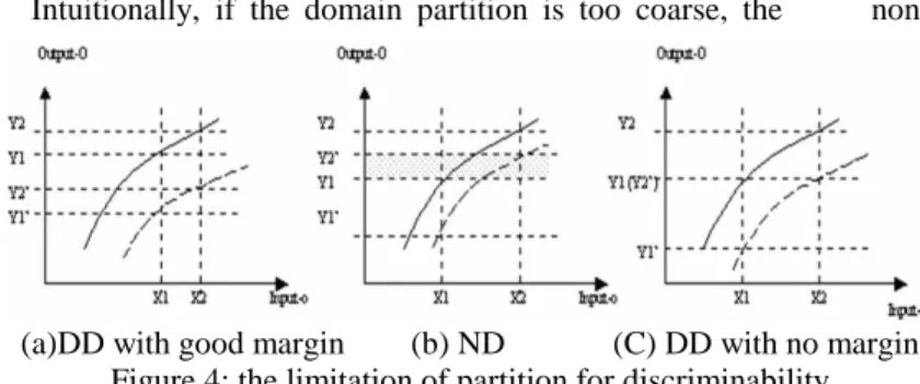
Intuitionally, if the domain partition is too coarse, the
output ranges of the two modes will be overlapped. In this case, such that the two modes are undiscriminable (cf. figure 4). In other word, if the discrepancy between the two modes is larger, the domain partition can be coarser. Assume the two behavior modes have numeric models:
Y=f1(X) and Y=f2(X). MODELmode1 and MODELmode2 are
the qualitative models, so MODELmode1=q(f1) and
MODELmode2=q(f2). If ∃[X1 X2], q(f1): [X1 X2]→[Y1
Y2], q(f2):[X1 X2]→[Y1’ Y2’]. From proposition1, if
[Y1 Y2]obs [Y1’ Y2’]obs = Ø, (11)
1
This can be easily prove by assume PROJobs\cause
(MODELmode1 OPCi ) PROJobs\cause (MODELmode2 OPCi ) Ø. Since Vo-cause take the same value for mode1 and mode2, we have PROJobs (MODELmode1 OPCi ) PROJobs (MODELmode2 OPCi ) Ø , conflict.
The [X1 X2] belongs to DD range. In (11) the [Y1 Y2]obs
is the observables in [Y1 Y2]. This is the case in Figure4(a). If [Y1 Y2]obs [Y1’ Y2’]obs Ø (12)
The [X1 X2] belongs to non-DD range. This is the case in Figure4(b).
The limit between DD and non-DD is as Figure 2(c): [Y1 Y2]obs [Y1’ Y2’]obs = Y1’obs =Y2obs, or (13)
[Y1 Y2] obs [Y1’ Y2’]obs = Y2’obs =Y1obs (14)
Figure 4(c) is the coarsest partition for Vobs that still
keeps DD. It is easy to prove if the partition is coarser, the modes are non-DD2.
Corollary: The boundary of the coarsest partition is the
surface where the two modes joint.
For monotonic functions, the coarsest landmark is easy to compute:
Proposition 2: Assume MODELmode1 and MODELmode2
have quantitative models f1 and f2. f1 and f2 are monotonic. {X1, X2,…, Xi,…} are the input points. The coarsest
partition for Vo-cause satisfies
f1(X1) = f2(X2)
f1(X2) = f2(X3)
…
f1(Xi) = f2(Xi+1)
When Vo-cause get the coarsest partition {X1, X2,…, Xi,…}obs, Vobs\cause get the coarsest partition {f1(X1),
f1(X2), …, f1(Xi), …}obs.
Proposition 2 provides a way to generate new landmarks. It is possible to numerically compute Xi+1 from Xi. For
non-monotonic functions, proposition 2 does not hold. In the next section, a non-optimal but satisfactory solution of landmark generation is presented.
Model Abstraction with Landmark
Generation
The method presented in this section is relied on one fact that if the domain partition is finer, the discriminability can be improved. X = f(t) is a dynamic system. The simulation time is from 0 to Tc. The algorithm 2 starts from the coarsest
landmark [LOC1, LOC2], in which LOC1 and LOC2is the
lower bound and upper bound of Xo-cause. From the
simulation data, the discriminability on [LOC1, LOC2] is
examined (based on Proposition 1). If [LOC1, LOC2] is not
a DD range, that might mean that this partition is too coarse. [LOC1, LOC2] is split from the medium point, i.e.
(
LOC1+LOC2)/2
is added as a new landmark. [LOC1,(
LOC1+LOC2)/2
] and(
LOC1+LOC2)/2
, LOC2] are twointervals to be checked. The split process will continue until a DD scope is found, or the split makes the intervals smaller than a pre-defined minimum length D. Algorithm 2 records the generated landmarks, the qualitative relations,
2 Without loss of generality, assume f1 and f2 is monotonic as
figure 2(c), and f1(X1) = f2(X2). If Vo-cause has a larger partition
[X3, X2], where X3<X1, we get f1(X3)<f1(X1) = f2(X2) and f2(X3) < f2(X1)<f1(X1). Thus [f1(X3), f1(X2)] [f2(X3), f2(X2)] = [f1(x3),f1(x1)] Ø.
(a)DD with good margin (b) ND (C) DD with no margin Figure 4: the limitation of partition for discriminability
as well as the discriminability property on each input partitions.
Algorithm2: qualitative model abstraction X = f(t)
Input:
D: Minimum landmark interval Tc: duration of simulation time
f, f’: Quantitative models for two modes,
Vo-cause ={ xi | xi∈X}, Vobs\cause = { xj | xj∈X}, Vobs\cause ∪
Vo-cause ⊆ X
[LOC1, LOC2]: the start landmark for Vo-cause, i.e. LOC1=f o-cause(0), LOC2= fo-cause(Tc)
Output:
DD: Vector for input scope that system are DD
ND: Vector for input scope that system are non-DD (PD or ND)
q: Vector for storing qualitative model
loop: the Boolean variable controls loop, initialized as true Internal Variables:
p: stack to store input tuples
1: Store [LOC1, LOC2] in p
2: While p is not empty
3: pop a tuple [LOCi, LOCi+1] from p
4: find ti and ti+1 correspondent to LOCi, LOCi+1
5: LONCi = min{fobs\cause(t)| ti <t<ti+1}
6: LONCi+1 = max{fobs\cause(t)| ti <t<ti+1}
7: LONCi’= min{f’obs\cause(t)| ti <t<ti+1}
8: LONCi+1’= max{f’obs\cause(t ti <t<ti+1}
9: if [LONCi, LONCi+1]∩ [LONCi’, LONCi+1’] = ∅,
(that means [LOCi, LOCi+1] is in DD scope)
10: store [LOCi, LOCi+1] in vector DD
12: store {[ min{f(t)| ti <t<ti+1}, max{f(t)| ti < t <
ti+1}]} in vector q
13: remove [LOCi, LOCi+1] from p
14: else
15: mid = (LOCi+LOCi+1)/2
16: if | LOCi- mid|<=D or |LOCi+1 -mid| <=D
17: store {[min{f(t)| ti<t<ti+1}, max{f(t)| ti< t <
ti+1}]} in vector q
18: store [LOCi, LOCi+1] in vector ND
19: remove [LOCi, LOCi+1] from p
20: else
21: push [LOCi, mid] and [mid, LOCi+1] into q
22: end-if 23: end-if 24: end-while 25: report DD,ND, q
The key issue for algorithm 2 is the splitting procedure that refines the qualitative relation until to the level the fault is discriminable.
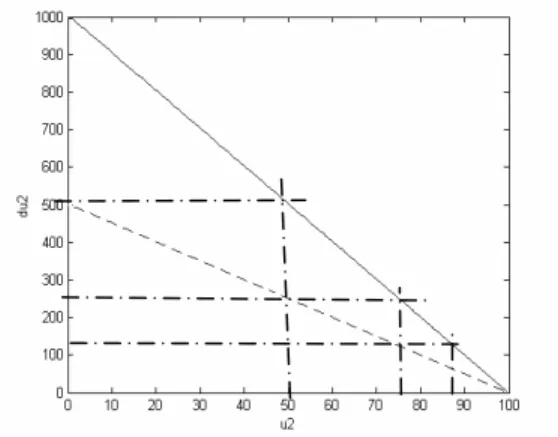
Resume the RC example in section 3.3. The voltage u1,
u2, and u3 are measurable observables. du2, the derivative
of u2, is the pseudo variable and is also a supplementary observable. The fault considered is the resistance of the resistor doubled, which causes the transient process slower.
u1 and u3 are constant (u1 = 100v, u3 = 0v) in this
example. u2 is chosen as Vo-cause, and du2 as Vobs\cause.
Figure 5 is the relation of u2 and du2 under the right (solid line) and faulty modes (doted line). Using algorithm 2, the split process is like figure 5.
Some comments on algorithm 2:
1. the partitions obtained from algorithm 2 are not the coarsest but the satisfactory one for diagnosis purpose. It is the
trade-off of optimization and computation cost.
2. the success of algorithm 2 depends on the selection of the variables to be split. Normally the most influential variables are chosen as the base variables. The split of the base variables can cause the largest change on the output variables. It needs special techniques to determine which variables are the most influential variables. The causal ordering algorithm [Iwasaki and Simon, 1994] can be used for this purpose. The base variables used in the RC circuit and in the demonstration case in this paper are selected by experience.
3. For the monotonic functions, the refinement of domain partition always refines the distinctions of Vobs\cause. For the
non-monotonic functions, it is not true due to the local extrema. But it is sure that the partition refinement doesn’t remove the distinctions of Vobs\cause.
4. This algorithm considers only partitions on continuous variables. For discrete variables, normally we regard them as different operation mode. For example: the switch can be on and off. They are considered as two operation modes. Thus this algorithm is suitable for most of the system. 5. For continuous variable, the valid value is bounded by working environment. For example, for a normal AC system, we consider the outside temperature is from –20 to 40.
Demonstration
(R=100ohm, C=0.001F for the right mode, and R=200ohm C=0.001F for the faulty mode)
Table 1 Landmarks for p1 and dp2 (a) Matlan/SimulinkModel Blower Distribution p0, f0,E p1, f1 Cabin p2, f2 p3, f3
(b) Model in block diagram Figure 6: AC system with 3 components
A simple Air Conditioning system has 3 components, Blower, Distribution and Cabin (figure 6). Figure 6(a) is the model in Matlab/Simulink, while figure 6(b) is in block schema with the input and output variables for each block. pi is pressure, fi is airflow rate, E is the electricity power
driving the blower. The flow rate and pressure inside the system increase when the blower begins to work, and they reach a stable point when E is unchanged. If the cabin volume increases, the transient procedure is slower than normal case but the same stable point can be reached. It is difficult to manually determine the landmarks for the variables. The algorithm 2 can deal it with. Suppose we can measure any pressure if necessary because normally pressure is easier to measure than flow rate. Since we already know p0 and p3 are equal to outside air pressure, they have no influence on diagnosability. Consider Vo={p1,
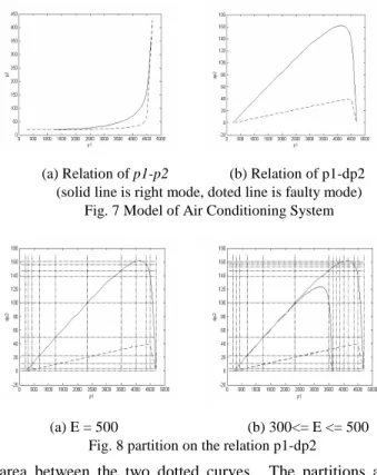
p2, dp2}, where dp2 is the derivative of p2. The relations of p1-p2 and p1-dp2 are drawn from simulation data as in Figure 7, where the solid curve is for the right mode and the doted line is for the faulty mode. One can see that the relations of p1-p2 at the two modes are too close to distinguish the two modes, but the relations of p1-dp2 have good distance to each other. And if p1 is the base variable to be split, the two modes can be distinguished. We choose Vo-cause = {p1} and Vobs\cause = {p2, dp2}. The landmarks
for p1 and dp2 are listed in table 1. Figure 8 shows the partitions on p1-dp2. Figure 8(a) is the result of 6 times of split. Except the most right and left interval of p1, the other intervals are Deterministic Diagnosable region. The landmarks of other variables are computed accordingly, which are not showed
in this paper. Figure 8(b) shows the partition result when E changes. The two solid curves are for E = 500 and E = 300 respectively. The area between the two curves are the right behaviour when 300 <= E <=500. The faulty mode is the
area between the two dotted curves. The partitions are result after 6 split. One can see that after p1>3500, the refinement of landmarks does not help to increase the diagnosability. For the algorithm 2, the split continues and generates some landmarks that do not help to distinguish the fault.
Discussion and conclusion
This paper bridges the gap between the numeric simulation model and the qualitative model for diagnosis purposes. The problem can be classified into four classes: 1) known landmark, static system; 2) known landmark, dynamic system; 3) unknown landmark, static system; 4) unknown landmark, dynamic system. The first class can be solved by algorithm 1. The performance of algorithm 1 is discussed in section 3.2. The second class can be transformed to the first class if the time information is eliminated from the simulation data. Similarly, the fourth class can be transformed to the third class in this way. For the third class, this paper reveals the relation of discriminability and model partition. The approximation of the qualitative model should keep the distinctions between the right and faulty behaviours. Beginning with the coarsest domain partition, algorithm 2 is a refining process, generating new landmarks until the target modes can be distinguished at the new, finer partitions.
Algorithm 2 can be used as a generalized approach for both static and dynamic systems and both monotonic and non-monotonic cases. Algorithm 2 is limited in two ways. First only single fault is considered. This needs further
p1 dp2 209.7617 307.2409 446.2227 697.8665 1246.9854 2326.6505 3491.1238 4019.3584 4350.6848 4498.3403 4690.4157 0.3072 4.4389 11.2196 22.7634 49.7219 99.5160 147.2230 160.8867 156.5737 138.0294 0.0
(a) Relation of p1-p2 (b) Relation of p1-dp2 (solid line is right mode, doted line is faulty mode)
Fig. 7 Model of Air Conditioning System
(a) E = 500 (b) 300<= E <= 500 Fig. 8 partition on the relation p1-dp2
work, but the principles developed here can be used. Secondly, the approach is system-context dependent and diagnosis task dependent. That means the abstracted qualitative model depends on the current system structure and the considered fault. If the component model is reused in another system context or to diagnose other faults, we can not guarantee the fault is detectable. This is a compromise of data explosion because theoretically a universal qualitative model contains an unlimited amount of information, which is unable to be described by finite domains. After this project, we believe no universal qualitative model exists. The only feasible way is to get a qualitative model under certain conditions. Based on this, our algorithm has many advantages: first it is a one-step method. By running one process, all component models are obtained. Practically it is not a big deal to run it on each system even if the component model is not reusable. Second the considered fault is guaranteed to be detected using the resulted model. Third it avoids possible conflicts when the shared variables among components are no in the same scope if the component models are collected one by one. From our experience, this approach is very practical in dealing with complex real-world industrial applications.
References
Brooks, M. 1984., Approximation Complexity for Piecewise Monotone Functions and Real Data. Computers
and Mathematics with Applications 27(8).
Dressler, O. 1996. On-line Diagnosis and Monitoring of Dynamic Systems based on Qualitative Models and Dependency-recording Diagnosis Engines, in Proceedings of the 12th European Conference on Artificial Intelligence, 481-485.
Dupre, D. and Panati, A. 1998. State-based vs simulation-based diagnosis of dynamic systems. In Proceedings of the 9th International Workshop on Principles of Diagnosis, 40-46.
Dvorak, D. and Kuipers, B. 1992. Model-based Monitoring of Dynamic Systems, in Readings in Model-based
Diagnosis: 249-254. Morgan Kaufmann Publishers.
Iwasaki, Y. and Simon, H. 1994. Causality and Model Abstraction. Artificial Intelligence 67(1):143-194.
Karnopp D. and Rosenberg, R. 1975, System Dynamics: A
Unified Approach, John Wiley & Sons, Inc.
Kuipers, B. 2001. Qualitative Simulation. In R.A. Moyers (Ed.) Encyclopedia of Physical Science and Technology, Third Edition, NY Academic Press.
Lunze, J., Nixdorf, B. and Schreoder, J. 1999. Deter-ministic Discrete-event Representations of Linear Continuous-variable Systems, Automatic 35:395-406. Malik, A. and Struss, P. 1996. Diagnosis of Dynamic Systems Does Not Necessarily Require Simulation. In Proceedings of the 10th International Workshop on Qualitative Reasoning, 127-136.
Mosterman, P. and Biswas G. 1997. Model Based Dia-gnosis of Dynamic System. In Seventh Journees de
L.I.P.N.,134-154, University of Paris Nord, Villetaneuse, France.
Panati, A. and Dupre, D. 2000. State-based vs simulation-based diagnosis of dynamic systems. In Proceedings of the 14th European Conference on Artificial Intelligence, 176-180.
Sachenbacher, M. and Struss, P. 2001. AQUA : A Frame-work for Automated Qualitative Abstraction. In Proceedings of 15th International Workshop on Qualitative Reasoning, 5-12.
Schit, C. and Bredeweg, B. 1996. An overview of approaches to qualitative Model Construction. The
Knowledge Engineering Review 11(1):1-25.
Struss, P., Refus, B., Cascio, F., Console, L. Dague, P., Dubois, P., Dressler, O., and Millet, D. 2002. Model-based Tools for the Integration of Design and Diagnosis into a Common Process – A Project Report. In Proceedings of 13th International Workshop on Principles of Diagnosis, 25-32.
Struss, P. 1997. Fundamentals of Model-Based Diagnosis of Dynamic Systems. In Proceeding of the 15th Inter-national Joint Conference on Artificial Intelligence, 480-485.
Struss, P. 2002. Automated Abstraction of Numerical Simulation Models – Theory and Practical Experience. In Proceedings of Sixteenth International Workshop on Qualitative Reasoning, p161-168.