Caisson structures in the Beaufort Sea 1982-1990 : Characteristics, instrumentation and ice loads

(1)

Publisher’s version / Version de l'éditeur: Technical Report, 2002-11

READ THESE TERMS AND CONDITIONS CAREFULLY BEFORE USING THIS WEBSITE. https://nrc-publications.canada.ca/eng/copyright

Vous avez des questions? Nous pouvons vous aider. Pour communiquer directement avec un auteur, consultez la

première page de la revue dans laquelle son article a été publié afin de trouver ses coordonnées. Si vous n’arrivez pas à les repérer, communiquez avec nous à PublicationsArchive-ArchivesPublications@nrc-cnrc.gc.ca.

Questions? Contact the NRC Publications Archive team at

PublicationsArchive-ArchivesPublications@nrc-cnrc.gc.ca. If you wish to email the authors directly, please see the first page of the publication for their contact information.

Archives des publications du CNRC

For the publisher’s version, please access the DOI link below./ Pour consulter la version de l’éditeur, utilisez le lien DOI ci-dessous.

https://doi.org/10.4224/12328162

Access and use of this website and the material on it are subject to the Terms and Conditions set forth at Caisson structures in the Beaufort Sea 1982-1990 : Characteristics, instrumentation and ice loads

Timco, G. W.; Johnston, M. E.

https://publications-cnrc.canada.ca/fra/droits

L’accès à ce site Web et l’utilisation de son contenu sont assujettis aux conditions présentées dans le site LISEZ CES CONDITIONS ATTENTIVEMENT AVANT D’UTILISER CE SITE WEB.

NRC Publications Record / Notice d'Archives des publications de CNRC:

https://nrc-publications.canada.ca/eng/view/object/?id=fa717e43-d8c5-44bb-af82-fb1040ed783c https://publications-cnrc.canada.ca/fra/voir/objet/?id=fa717e43-d8c5-44bb-af82-fb1040ed783c

(2)

Caisson Structures in the Beaufort Sea 1982-1990:

Characteristics, Instrumentation and Ice Loads

G.W. Timco and M.E. Johnston Canadian Hydraulics Centre National Research Council of Canada

Ottawa, Ont. K1A 0R6 Canada

Technical Report CHC-TR-003

(3)

(4)

Caisson Structures in the Beaufort Sea

G.W. Timco and M.E. Johnston CHC-TR-003 Page 1

ABSTRACT

This report presents a comprehensive overview of the characteristics, instrumentation and measured ice loads on the caisson structures that were used for exploratory drilling in the Canadian Beaufort Sea in the 1970s and 1980s. Details are presented on the Tarsiut Caissons, the Single Steel Drilling Caisson (SSDC), the Caisson Retained Island (CRI), and the Molikpaq. Details on the ice-load measuring instrumentation are presented for each of the drill sites where an ice-load measurement program took place. The global loads on the structures are presented as a Line Load (Global Load per width of the structure) and the Global Pressure (Line Load per ice thickness). Global loads are shown to be a function of the ice macrostructure (level year sea ice, multi-year ice, first-year ridges, hummock fields, isolated floes). The analysis shows that there is a general increase in the Line Load with increasing ice thickness. The data show considerable scatter. Much of the scatter can be explained by examining the failure mode of the ice during the interaction process. The most significant result of the analysis shows that the maximum Global Pressure measured for all types of ice loading events never exceeded 2 MN/m2.

(5)

(6)

TABLE OF CONTENTS ABSTRACT ... 1 TABLE OF CONTENTS ... 3 LIST OF FIGURES ... 5 LIST OF TABLES ... 8 1.0 INTRODUCTION... 9

2.0 OVERVIEW OF BEAUFORT SEA STRUCTURES ... 10

2.1 Artificial Islands ... 10

2.2 Floating Drillships ... 10

2.3 Caisson Structures ... 13

2.4 Spray Islands ... 13

2.5 Overview of Drilling Activity... 15

2.6 Definition of Terms ... 18

3.0 TARSIUT CAISSONS ... 20

3.1 Description of the Tarsiut Structure ... 20

3.2 Instrumentation on the Tarsiut Structure ... 20

3.3 Tarsiut Ice Loading Events ... 22

4.0 SINGLE STEEL DRILLING CAISSON (SSDC) ... 24

4.1 Description of the SSDC... 24

4.2 SSDC Instrumentation and Ice Loads... 25

4.2.1 Uviluk Site, 1982 – 83 ... 26

4.2.2 Kogyuk Site, 1983 – 84... 26

4.2.3 Phoenix Site, 1986 – 87 ... 27

4.2.4 Aurora Site, 1987 - 88... 30

4.2.5 Overview of Ice Loads on the SSDC ... 32

5.0 CAISSON-RETAINED ISLAND (CRI) ... 33

5.1 Description of the CRI ... 33

5.2 Hull Instrumentation on the CRI ... 33

5.3 Field Instrumentation and Ice Loads on the CRI ... 35

5.3.1 Kadluk, 1983-84 ... 35

5.3.2 Amerk, 1984-85... 37

5.3.3 Kaubvik, 1986-87 ... 39

5.4 Overview of Ice Loads on the CRI ... 44

6.0 MOLIKPAQ... 45

6.1 Description of the Molikpaq ... 45

6.2 Instrumentation on the Molikpaq ... 46

6.3 Calculation of Load ... 50

6.4 Ice Conditions and Molikpaq Events... 51

6.4.1 Tarsiut P-45 ... 51

6.4.2 Amauligak I-65... 52

6.4.3 Amauligak F-24 ... 52

6.4.4 Isserk I-15... 52

(7)

7.0 GLOMAR BEAUFORT SEA 1 (CIDS)... 57

7.1 Overview of Ice Loads on the CIDS ... 57

8.0 DISCUSSION ... 58

8.1 Level First-year Sea Ice ... 58

8.1.1 Influence of Floating Rubble ... 58

8.1.2 Failure Modes ... 60

8.2 Ice Macrostructure... 65

9.0 SUMMARY ... 69

(8)

LIST OF FIGURES

Figure 1: Photograph of sandbag protected artificial island... 11

Figure 2: Photograph of the Esso artificial island at Issungnak ... 11

Figure 3: Photograph of a Canmar drillship ... 12

Figure 4: Photograph showing the ice management around the moored Kulluk structure in the Beaufort Sea. ... 12

Figure 5: Photograph showing an overview of the Nipterk spray island. ... 14

Figure 6: Photograph showing the Nipterk spray island from ice level... 14

Figure 7: Overview of drilling activity in the Canadian Beaufort Sea. ... 17

Figure 8: Map showing the gas and oil discoveries in the Canadian Beaufort Sea (after Jahns 1985). ... 18

Figure 9: Side view through Tarsiut caisson structure... 20

Figure 10: Illustration of MEDOF panel locations surrounding Tarsiut caisson during the 1982/83 season... 22

Figure 11: Overhead view of Tarsiut Caisson showing the grounded rubble field surrounding the structure (photo taken on March 2, 1983). ... 23

Figure 12: Line-Load on the Tarsiut Caisson as a function of ice thickness. Note that in all cases there was a 150 m grounded rubble field surrounding the structure. ... 23

Figure 13: SSDC at the Kogyuk site in the Beaufort Sea. Note the sprayed ice rubble surrounding the structure. ... 24

Figure 14: Artist's cut-away illustration of the SSDC and the MAT... 25

Figure 15: Dimensions of the SSDC and the MAT ... 25

Figure 16: Location of the load measuring sensors on the SSDC at the Uviluk site. ... 26

Figure 17: Location of instrumentation in the ice surrounding the SSDC/MAT at the Phoenix site (1986-87). ... 28

Figure 18: Photograph of the SSDC at the Phoenix site. Note the large rubble field surrounding the structure. ... 30

Figure 19: Location of instrumentation in the ice surrounding the SSDC/MAT at the Aurora site (1987-88). ... 31

Figure 20: Line Load on the SSDC as a function of the ice thickness. ... 32

Figure 21: Illustration of the Caisson Retained Island (after Croasdale, 1985) ... 33

Figure 22: Illustration of the location of the instrumentation on the hull of the CRI. ... 35

Figure 23: Ice conditions and instrumentation at Kadluk, spring 1984 (after Johnson et al., 1985 with adaptations)... 36

Figure 24: Ice rubble surrounding the CRI at the Amerk site. ... 38

Figure 25: Instrumentation around the CRI at the Amerk site. ... 38

Figure 26: Stress measured on Panel 7 at the Amerk site from March 27 to April 27, 1985 (after Sayed et al., 1986 with adaptations) ... 39

Figure 27: Photograph of the grounded rubble field around the CRI at the Kaubvik site.40 Figure 28: Location of the in-situ stress sensors in the rubble field surrounding the CRI at the Kaubvik site... 41

(9)

Figure 29: Late winter map of rubble extent around the CRI-Kaubvik showing location of BP-type sensors (after Frederking and Sayed, 1988; Marshall, 1990; with adaptations). ... 42 Figure 30: Output from the in-situ load panels installed around the CRI at Kaubvik (after Frederking and Sayed, 1988 with adaptations)... 43 Figure 31: Output from the BP-type sensors installed south of the CRI at Kaubvik (after Marshal, 1990 with adaptations). ... 44 Figure 32: Photograph of the Molikpaq in the Canadian Beaufort Sea. ... 45 Figure 33: Cross-section view of the Molikpaq at the Amauligak I-65 site in 1985-86... 46 Figure 34: General location of the MEDOF panels on the Molikpaq. Each MEDOF panel sensor group has a sensing width of two panels, each 1.135 m wide and 2.7 m high. The detailed locations of individual panels are shown in Figure 34... 47 Figure 35: Location of the individual MEDOF panels on the Molikpaq. ... 48 Figure 36: Locations of the 16 SG09 strain gauges on the Molikpaq. ... 49 Figure 37: Line Load versus ice thickness on the Molikpaq. This plot shows only data relevant to level, first-year sea ice... 54 Figure 38: Line Load as a function of ice thickness for multi-year ice interacting with the Molikpaq... 54 Figure 39: Line Load as a function of sail height for first-year ridge interaction with the Molikpaq... 55 Figure 40: Line Load as a function of the host ice thickness for first-year hummock ice.55 Figure 41: Line Load as a function of the average ice thickness of large isolated floes impacting the Molikpaq. The graph shows data for both first-year and multi-year ice. ... 56 Figure 42: Photograph of the CIDS in ice. ... 57 Figure 43: Line Load as a function of ice thickness for first-year level ice. The figure shows that there is little influence of floating rubble on the loads on the structure.. 59 Figure 44: Global Pressure versus ice thickness for level first-year sea ice. ... 59 Figure 45: Crushing along the corner of the Molikpaq. Note that the large build-up of ice rubble has caused a subsequent large flexural failure of the ice sheet... 60 Figure 46: Local flexural failures along the side of the Molikpaq. ... 61 Figure 47: Mixed mode failure along the side of the Molikpaq. Note the large cracks in the parent ice sheet. ... 61 Figure 48: Pile-up alongside the Molikpaq. ... 62 Figure 49: Line Load as a function of ice thickness showing the influence of the failure mode of the ice on the measured load. ... 62 Figure 50: Global Pressure versus the time-to-failure for first-year sea ice. ... 63 Figure 51: Global Pressure versus the average loading rate for first-year level sea ice. .. 63 Figure 52: Line Load as a function of the host ice thickness for first-year hummock ice showing the associated failure modes for the ice... 64 Figure 53: Line Load as a function of the floe ice thickness for first-year isolated floes showing the associated failure modes for the ice... 65 Figure 54: Line Load as a function of ice thickness for different ice macrostructures for first-year ice only. ... 66 Figure 55: Line Load as a function of ice thickness for different ice macrostructure for both first-year and multi-year ice. ... 67

(10)

Figure 56: Global Pressure as a function of ice thickness for different ice macrostructure for first-year ice only. ... 67 Figure 57: Global Pressure as a function of ice thickness for different ice macrostructure for both first-year and multi-year ice. ... 68

(11)

LIST OF TABLES

Table 1: Details of the Fixed Structures used in Arctic Drilling ... 13

Table 2: Drilling Activity in the Canadian Beaufort Sea ... 15

Table 3: Details of the Molikpaq deployment in the Beaufort Sea. ... 46

(12)

Caisson Structures in the Beaufort Sea 1982-1990:

Characteristics, Instrumentation and Ice Loads

1.0 INTRODUCTION

During the 1970s and 1980s there was considerable activity for oil exploration in the Canadian and American Beaufort Sea. Over 140 wells were drilled using innovative technology that evolved with time. This evolution was a result of a better understanding of the Arctic environment and the need to operate in increasingly deeper waters with more extreme ice conditions. Initially during this exploration, the knowledge of actual ice loads on wide structures was virtually non-existent. Because of this, many of the structures were instrumented to measure the ice loads, and active and invaluable measurement programs were developed.

When the Beaufort Sea activity declined in the early 1990s, the Oil Industry redirected its interests to other regions. Since there was a fear that the information and knowledge of the ice loads might be lost, the National Research Council in Ottawa approached the Oil Industry to gain access to, archive, and use this information. The Industry was very responsive to this request and the NRC set-up a Centre of Ice Loads on Structures (Timco 1996, 1998). The Program on Energy Research and Development (PERD) provided funding for this project. The NRC obtained reports, data, and videos from Gulf Canada Resources Ltd., Imperial Esso, and Dome Petroleum (Canmar). At the present time, there are over 2000 reports, 300 films and videos, and original data from the Molikpaq and the Single Steel Drilling Caisson (SSDC). The NRC actively uses this information to better understand ice loads on offshore structures (Frederking et al., 1999; Timco et al., 1999a, 1999b; Timco and Wright, 1999; Wright and Timco, 2000).

Recently, there has been interest in continuing exploration of the Beaufort Sea. The intent of this report is to provide an overview of the drilling activity in the 1980s and 1990s. Particular emphasis is given to the ice loads measured on the caisson-type structures.

(13)

2.0 OVERVIEW OF BEAUFORT SEA STRUCTURES

There have been several approaches used to design platforms for oil exploration in the Arctic regions. In the Beaufort Sea, off both Canada and Alaska, over 140 wells have been drilled. Innovative technology and good management have allowed exploration of this region. The exploration took place over a fairly short time span. A number of the major oil companies were involved in this venture. There was both competition and collaborative work to investigate the ice loads and types of structures that could be used. This section details the structures that were used.

2.1 Artificial Islands

The development of the Beaufort was initiated in the early 1970s in quite shallow water (up to 12 m) using artificial islands. These islands were constructed by either dredging the local sea bottom and building-up an island, or by trucking gravel from the shore and dumping it to form an island. For most of these islands, the ice was landfast, first-year ice and had little movement during the winter months. In the early 1970s, Esso Resources Canada Ltd. and Exxon Production Research measured the in-situ ice pressures around their dredged exploration drilling islands at Adgo, Netserk, Arnak, Kannerk and Issungnak (see Figure 1 and Figure 2). Urethane button-type sensors were used to measure the pressure, with supplementary information on ice/island movements. These measurement programs often experienced electrical and environmental difficulties and little data are available from them in the open literature. The successful measurements indicated, however, that the ice load was applied relatively uniformly across the Island, with loading times on the order of one day. The field studies indicated that pressures up to about 1 MPa were measured on this type of structure (Ralston, 1979).

2.2 Floating Drillships

Starting in the mid 1970s, Dome Petroleum (Canmar) deployed floating drillships during the summer months (Figure 3). These were moored on site during the summer (open water) months. They encountered relatively light ice conditions, and there are no recorded ice loading events for these floating structures.

In 1983, Gulf Canada Resources Ltd. designed and built an inverted-cone shaped floating structure (the “Kulluk”) that allowed drilling later into the winter season. This structure was exposed to moving pack ice. Active ice management around the Kulluk ensured that the ice conditions were not severe (see Figure 4). This structure was instrumented to measure mooring line forces. Wright (2000, 2001) summarized the measured forces on the Kulluk. Measured loads were up to 4 MN depending upon the ice thickness, floe size and ice concentration.

(14)

Figure 1: Photograph of sandbag protected artificial island

(15)

Figure 3: Photograph of a Canmar drillship

Figure 4: Photograph showing the ice management around the moored Kulluk structure in the Beaufort Sea.

(16)

2.3 Caisson Structures

In the early 1980s, five special-built caisson structures were designed and built to allow year-round drilling and development of regions further offshore in harsher ice conditions. There were five different caisson structures used in Arctic regions:

§ Tarsiut Caisson

§ Single-Steel Drilling Caisson (SSDC) § Caisson-Retained Island (CRI)

§ Molikpaq

§ Glomar Beaufort Sea I (CIDS)

Table 1 provides some details on their characteristics, based on the paper by Masterson et al. (1991). The caisson structures are discussed in detail in later chapters of this report.

Table 1: Details of the Fixed Structures used in Arctic Drilling

Tarsiut SSDC CRI Molikpaq CIDS

Drilling Days (per year) 365 365 365 365 365

Base Area (m2) 7947 18590 10875 12383 8551

(including core)

Oceanographic Limitations 12 12.2 15 12.2 5.2

(wave height - m)

Limiting Level Ice Conditions (m) 5.6 10 3 10 2

Ice Concentrations 10/10s 10/10s 10/10s 10/10s 10/10s

Design Ice Load - Global (MN) 560 900 436 640 640

Design Local Ice Pressure (MPa) 4.1 8.3 2.8 3.0 6.2

Area for Local Pressure (m2) 3.7 3.7 0.7 2.3 2.3

Wells Drilled Tarsiut N-44 Uviluk P-66 Kadluk O-07 Tarsuit P-45 Antares #1 Tarsiut N-44A Kogyuk N-67 Amerk O-09 Amauligak I-65 Antares #2

Phoenix #1 Kaubvik I-43 Amauligak I-65A Orion #1

Aurora #1 Amauligak I-65B

Amauligak 2F-24 Amauligak 2F-24A Amauligak F-24 Amauligak 2F-24B Isserk I-15 2.4 Spray Islands

In the late 1980s, spray ice islands (Figure 5 and Figure 6 after Poplin, 1990) were used for a few wells. These were deployed in landfast ice in both the Alaskan and Canadian Beaufort Sea. The cost of these spray islands was approximately one-half the cost of a gravel island.

(17)

Figure 5: Photograph showing an overview of the Nipterk spray island.

(18)

2.5 Overview of Drilling Activity

There were 88 wells drilled in the Canadian Beaufort Sea. Table 2 lists some of the salient details of these wells (from Masterson et al., 1991).

Table 2: Drilling Activity in the Canadian Beaufort Sea

Year Well Name Operator Drill Vessel Water Depth (m) Spud Date Rig Release

1972 Roland Bay L-41 Pacific --- 20.1 72/12/22 73/04/20

1973 Immerk B-48 Imp Sacrificial beach 3.0 73/09/17 73/12/22

Adgo F-28 Esso Sandbag retained 2.0 73/12/28 74/03/19

1974 Pullen E-17 Imp Sandbag retained 1.5 74/04/21 74/07/11

Unark L-24 Sun/BVX Hauled Island 1.5 74/09/26 75/05/24

Pelly B-35 Sun/BVX Hauled Island 1.5 74/11/05 75/02/14

1975 Adgo P-25 Esso Sandbag retained 2.0 75/01/02 75/03/28

Nerlerk B-44 Imp Sandbag retained 4.6 75/01/06 75/06/08

Adgo C-15 Esso Sandbag retained 2.0 75/04/21 75/07/25

Garry P-94 Sun/SOBC/BVX Hauled Island 2.5 75/08/25 76/01/05

Ikattok J-17 Imp/Delta Sandbag retained 2.0 75/10/07 76/02/28

Nerlerk F-40 Imp Sandbag retained 7.0 75/11/08 76/05/09

1976 Sarpik B-35 Imp Sandbag retained 3.5 76/04/02 76/09/04

Kopanoar D-14 Hunt/Dome Drill Ship 60.3 76/08/08 76/09/26

Nektoralik K-59 Dome/Hunt Drill Ship 34.0 76/09/21 77/10/17

Kugmallit H-59 Imp Sandbag retained 5.2 76/09/30 76/11/10

Arnak L-30 Imp Sacrificial beach 8.5 76/10/05 77/03/16

Tingmiark K-91 Dome/Gulf Drill Ship 27.3 76/10/18 77/10/25

Unark L-24A Sun/BVX Hauled Island 1.5 76/10/19 77/05/08

1977 Kannerk G-42 Imp/IOE Sacrificial beach 8.0 77/03/30 77/05/13

Ukalerk C-50 Dome/Gulf Drill Ship 20.0 77/07/18 77/10/03

Kopanoar M-13 Dome Drill Ship 59.5 77/07/19 79/xx/xx

Nerlerk M-98 Dome Drill Ship 52.0 77/10/07 79/08/28

Isserk E-27 Esso Sacrificial beach 13.0 77/12/04 78/05/05

1978 Garry G-07 Sun/CCL/BVX Hauled Island 2.5 78/02/10 78/05/13

Natsek E-56 Dome//Petrocan Drill Ship 34.1 78/07/10 79/10/16

Ukalerk 2C-50 Dome/Gulf Drill Ship 20.0 78/08/10 79/10/11

Tarsuit A-25 Gulf Drill Ship 20.0 78/10/18 80/07/28

Kaglulik M-64 Dome Drill ship 31.0 78/11/03 79/07/10

Kaglulik A-75 Dome Drill ship 32.6 78/xx/xx 78/xx/xx

1979 Adgo J-27 Esso Sandbag retained 2.0 79/04/05 79/08/07

Kenalooak J-94 Dome Drill ship 49.3 79/09/20 82/11/01

Kopanoar L-34 Dome Drill Ship 60.0 79/10/11 79/11/25

Koakoak O-22 Dome Drill ship 49.2 79/11/05 81/10/31

Kopanoar 2L-34 Dome/Gulf Drill Ship 60.3 79/11/25 79/11/28

1980 Kilannik A-77 Dome Drill ship 23.7 80/06/23 81/09/04

Kapanoar I -44 Dome/Gulf/Hunt Drill Ship 58.0 80/07/10 80/08/01

Kopanoar 2I-44 Dome/Gulf Drill Ship 57.9 80/08/03 80/10/29

Issungnak 2 O-61 Esso Sacrificial beach 18.6 80/10/02 81/08/13

1981 Issugnak L-86 Gulf Drill ship 18.6 81/07/17 81/10/16

Alerk P-23 Esso Sacrificial beach 11.6 81/09/21 81/12/24

Irkaluk B-35 Dome/Hunt Drill ship 60.3 81/09/28 82/10/04

(19)

Table 2 (cont’d): Drilling Activity in the Canadian Beaufort Sea

Year Well Name Operator Drill Vessel Water Depth (m) Spud Date Rig Release 1982 Issugnak O -61 Esso Sacrificial beach 36.5 82/02/06 80/07/08

West Atkinson L-17 Esso Sandbag retained 7.0 82/05/01 82/06/25

Tarsuit N-44A Gulf Caisson-concrete 19.2 82/06/18 82/09/19

Kiggavik A-43 gulf Drill ship 27.4 82/08/20 82/10/17

Orvilruk O-03 Dome/Superior Drill Ship 59.9 82/08/30 82/10/25

Aiverk I-45 Dome Drill ship 50.3 82/10/07 82/10/23

Aiverk 2I-45 Dome Drill ship 50.3 82/11/03 84/10/11

Itiyok I-27 Esso Sacrificial beach 14.0 82/11/05 83/05/02

Uviluk P-66 Dome/Texaco SSDC 30.0 82/11/10 83/05/21

1983 Natiak O-44 Dome Drill Ship 44.0 83/07/16 84/09/25

Havik B-41 Dome Drill ship 35.0 83/07/17 86/08/24

Siulik I-05 Dome Drill Ship 49.4 83/07/25 84/10/18

Arluk E-90 Dome Drill ship 58.0 83/07/30 85/10/13

Pitsiulak A-05 Gulf Kulluk 27.0 83/08/22 84/07/26

Kadluk O-07 Esso CRI 13.6 83/09/25 84/04/24

Kogyuk N-67 Gulf SSDC 28.4 83/10/28 84/01/30

Amauligak J-44 Gulf Kulluk 19.5 83/11/16 84/09/23

1984 Amerk O-09 Esso CRI 26.0 84/08/22 85/03/03

Nerlerk J-67 Dome Kulluk 45.0 84/09/16 85/10/24

Tarsuit P-45 Gulf Milikapq 22.4 84/09/25 84/12/24

Adgo H-29 Esso Sandbag retained 3.0 84/09/27 85/01/12

Nipterk L-19 Esso Sacrificial Beach 11.3 84/10/03 85/03/23

Akpak P-35 Gulf Kulluk 20.0 84/10/17 84/11/08

1985 Nipterk L-19A Esso Sacrificial Beach 11.3 85/04/21 85/07/15

Akpak 2P-35 Gulf Kulluk 20.0 85/06/10 85/07/07

Adlartok P-09 Dome Drill ship 67.4 85/08/08 85/10/17

Edlok K-56 N-56 Dome Drill ship 31.5 85/08/10 85/09/16

Amauligak I-65 Gulf Molikpaq 22.9 85/09/24 86/01/28

Adgo G-24 Esso Sandbag retained 1.4 85/10/07 86/01/07

Aagnerk E-56 Gulf Kulluk 20.0 85/10/28 86/06/26

Minuk I-53 Esso Sacrificial Beach 14.7 85/11/27 86/05/02

Ellice L-39 Chev/Tril Sandbag retained 2.0 85/xx/xx 86/04/20

1986 Amauligak I-65A Gulf Molikpaq 22.8 86/01/28 86/03/20

Amauligak I-65B Gulf Molikpaq 22.9 86/03/20 86/09/19

Arnak K-06 Esso Sacrificial beach 7.6 86/04/27 86/08/12

Kaubvik I-43 Esso/Home CRI 17.9 86/10/22 87/01/10

1987 Angasak L-03 Tril/Esso/Chevron Spray ice island 5.4 87/02/24 87/04/12

Amauligak 2F-24 Gulf Molikpaq 26.5 87/12/22 88/01/29

1988 Amauligak 2F-24A Gulf Molikpaq 26.6 88/01/30 88/02/17

Amauligak F-24 Gulf Molikpaq 26.6 88/04/13 88/08/12

Amauligak 2F-24B Gulf Molikpaq 26.6 88/04/15 88/08/07

Amauligak O-86 Gulf Kulluk 20.0 88/06/30 88/08/26

1989 Nipterk P-32 Esso/Chevron Spray Ice Island 6.7 89/02/21 89/04/20

Isserk I-15 Esso/Gulf Molikpaq 11.5 89/11/11 90/01/08

Kingark J-54 Amoco Drill ship 30.0 89/xx/xx 90/xx/xx

Figure 7 has been produced from the information in this table. It shows a “flow chart” overview of the drilling activity in the Canadian Beaufort Sea. Note the progression from seasonal artificial islands and drill ships to the more robust caisson-type structures.

(20)

G.W. Timco and M.E. Johnston

CHC -TR -003 Page 17 Amauligak I-65A Amauligak I-65B Akpak 2P-35 Aagnerk E-56 Nerlerk J-67 Akpak P-35 Pitsiulak A-05 Amauligak J-44 Koakoak O-22 Kopanoar 2L-34 Kaglulik M-64 Kaglulik A-75 Issugnak L-86 Irkaluk B-35 Kenalooak J-94 Kopanoar L-44 Natserk E-56 Ukalerk 2C-50 Tarsuit A-25 Ukalerk C-50 Kopanoar M-13 Kopanoar D-14 Nektoralik K-59 Minuk I-53 Nipterk L-19A Adgo H-29 Issugnak O-61 Kannerk G-42 Isserk E-27 Unark L-24A 1972 1973 1974 1975 1976 1977 1978 1979 1980 1981 1982 1983 1984 1985 1986 1987 Amauligak 2F-24A, 2F-24B Amauligak F-24, O-68 1988 Island Date Roland Bay L-41 Immerk B-48 Adgo F-28 Pullen E-17 Pelly B-35

Adgo P-25 Nerlerk B-44 Adgo C-15 Ikattok J-17 Nerlerk F-40 Sarpik B-35 Kugmallit H-59 Drill Ships Tingmiark K-91 Nerlerk M-98 Garry G-07 Adgo J-27 Kilannik A-77 Kopanoar I-44 Kopanoar 2I-44 Issungnak 2O-61 Alerk P-23 Tarsuit N-44 Tarsuit N-44 Kiggavik A-43 Orviluk O-03 Aiverk I-45 Aiverk 2I-45

Itiyok I-27 Uviluk P-66

Natiak O-44 Havik B-41 Siulik I-05 Arluk E-90 Tarsiut SSDC Caisson Retained Island Kulluk Molikpaq Kadluk O-07 Kogyuk N-67 Amerk O-09 Tarsuit P-45 Adlartok P-09

Edlok K-56, N-56 Amauligak I-65

Arnak K-06 _{Kaubvik I-43}

Angasak L-03 Amauligak 2F-24

1989 Nipterk P-32 Kingark J-54 Isserk I-15

Arnak L-30 West Atkinson L-17 Nipterk L-19 Adgo G-24 Ellice L-39 Garry P-94 Unark L-24

sacrificial beach island

spray ice island

hauled island

sandbag retained island

Notation

Figure

7

(21)

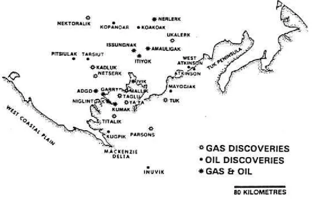
Significant oil and gas discoveries were made in the Beaufort Sea (see Figure 8), including the Amauligak oil reservoir. To date, these reserves have not been developed. Current discovered reserves for this region are 12 TCF gas, and 1.6 billion Bbls of oil. During the drilling of the Amauligak well, 320,000 barrels of oil were shipped to Japan in the tanker "Gulf Beaufort", making it the first major shipment of crude oil from the Canadian Beaufort Sea.

Figure 8: Map showing the gas and oil discoveries in the Canadian Beaufort Sea (after Jahns 1985).

2.6 Definition of Terms

As previously mentioned, the intent of this report is to provide an overview of the drilling activity in the 1980s and 1990s with particular emphasis on the ice loads on caisson-type structures. Before doing this, it is important to understand the format of the data presentation and define the approach that will be used.

The caisson structures were all quite wide (typically 100 m width). The measurement of loads was done by placing several sensors along the face of the structure. Then, by knowing the area covered and using extrapolation techniques, the loads were determined. For presentation here, these global loads were normalized by the width of the structure loaded by the ice. This is defined as a “Line Load” where

(22)

Ice the by loaded Structure of Width Load Global Measured Load Line =

Using this approach provides a coherent method to compare the data. Note that the measured global load was in most cases normalized by the full width of the structure at the waterline. In a few cases, the loads were measured over only one face of the caisson, and so the face width was used as the normalizing width.

In addition, the load information is presented by introducing the concept of a “Global Pressure”. This is defined as:

Thickness Ice x Ice the by loaded Structure of Width Load Global Measured essure Pr Global =

Thus, this is the Line Load normalized by the ice thickness. It should be emphasized that the values of Global Pressure should only be used in the context of the global loads on a structure. Local pressures would be considerably higher than the Global Pressure values reported here. This approach is used as a simple means to compile and compare the global load results for different structures and ice types.

(23)

3.0 TARSIUT CAISSONS

Gulf Canada Resources Ltd. operated this structure and it was the first caisson-type structure used in the Arctic. It drilled the Tarsiut N-44 well in 1981-82 (see Figure 8). During the winter of 1982-83, it was left on-site and used as a test platform to study ice interaction with a wide offshore structure. This project was known as the Tarsiut Island Research Program (TIRP).

3.1 Description of the Tarsiut Structure

The structure consists of four individual concrete caissons. These caissons were floated to the drilling site and ballasted down with sand to form a square. The inner core was filled with dredge material (see Figure 9). This structure is not regarded as a "mobile" structure since the difficulty of resetting and connecting four caissons limits its mobility. The structure is about 100 m across at the water line and has a vertical outer surface (Figure 10). The caissons are 10 m high and rest on a berm that comes to within 6 m of the water surface. The structure was extensively instrumented to measure ice loads (Pilkington et al., 1983) both for operational safety reasons and for future design.

Figure 9: Side view through Tarsiut caisson structure 3.2 Instrumentation on the Tarsiut Structure

Instrumentation comprised sensors to measure loads on the outer face, strain gauges embedded in the concrete and geotechnical sensors in the foundation and core. The strain gauges were of a weldable type and were attached to the steel reinforcing rods in the concrete. Gauge locations were selected on the basis of finite element calculations that also provided calibration coefficients for converting the measured strains to ice loads. From the location of the gauges, it was possible to establish load distributions and global loads. In spite of the care taken in the installation of gauges and cables, only a third of the gauges were operational at the beginning of the measurement program. Fortunately there was sufficient redundancy that useful results could still be obtained. A system of four 4 m by 4 m flat jack panels was attached to the outside of the east caisson. The outer face of each panel was an 89 mm thick steel plate to ensure that applied ice loads were uniformly distributed to the 16 flat jacks behind each panel. Pressure transducers measured the flat jack pressures.

(24)

Circular load cells were mounted in 880 mm diameter recesses in the north caisson. The sensing face was supported on shear bars or spiral coil hydraulic hoses. For more details on the characteristics of these transducers see Graham et al. (1983). The shear bar transducers had a number of desirable features (low temperature coefficient, no creep and high stiffness). The spiral coil transducers had less desirable features but were inexpensive. Unfortunately a storm in the autumn led to water entering these gauges and making a number of them inoperable. Finally, eight 50-mm diameter microstud gauges were installed in one of the flat jack panels to measure local pressures. These were a diaphragm type of pressure gauge.

Experience over the winter of 1981-82 showed that the embedded strain gauges and flat jacks provided consistent and reasonable ice load information. Inclinometers provided qualitative confirmation of major ice loading events and quantitative information for operational purposes.

During the winter of 1982-83, there was no drilling activity on the structure but it was left in place and used as a research platform. The island was manned with approximately 6 to 10 people, and measurements of ice loads, ice failure behavior and ice movements were made. The ice load measurements were primarily obtained from the output of a large number of MEDOF panels1 that were used to circle the structure (Figure 10). In addition, a few panels were placed further out in the grounded rubble field. During March to May, measurements were made by British Petroleum (BP) around the grounded rubble field (see Figure 11) to provide information on the local strain and strain rates in the adjacent ice sheet. Based on this information, the global loads on the island and rubble pile were inferred. A particular aspect of this work was the determination of the attenuation of loads through grounded rubble. In spite of the extensive work program, this question was not quantitatively answered.

1

MEDOF panels, which are 1.1 x 2.7 m in area, are a total load type of panel, i.e. they sense the total ice load on them. The contact area of the ice on the panel has to be estimated in order to determine the effective ice pressure. The panels can be deployed in either vertical or horizontal arrays, which allows local load distributions and global loads to be determined. They are a sandwich of two steel plates (inner plate about 2 mm thick and the outer plate is about 10 mm thick) over an array of polymeric buttons. The panels are closed at the edges and filled with a calcium chloride solution. Load application to the panel causes the buttons to compress and the internal volume of the panel to change. This volume change causes the calcium chloride fluid level in a stand pipe attached to the panel to change. A sensitive pressure transducer is used to measure the hydrostatic head changes in the standpipe. The maximum frequency response is estimated to be about 1 Hz.

(25)

MEDOF panels surrounding Tarsiut caisson 100 m 45 m 69 m 15 m

Figure 10: Illustration of MEDOF panel locations surrounding Tarsiut caisson during the 1982/83 season

3.3 Tarsiut Ice Loading Events

There were a number of different loading events defined for the 2 years that Tarsiut Island was deployed in the Beaufort Sea. The NRC Centre on Ice Loads (Timco 1996, 1998) has a complete set of reports that describe the measurement program and results. Although there were a number of different ice-loading events described in the reports, the information about them was not complete and often several assumptions were made in the calculation of the load. After reviewing the information, four ice-loading events were identified – one in 1981-82 and three from 1982-83. These are shown as a Line Load on the structure as a function of the ice thickness in Figure 12. In this approach, the measured global load has been normalized by the width of the structure being loaded by the ice. It should be noted that, although these were chosen as the best events, there was discrepancy in the estimated load by using different sensors and the time-series traces are very incomplete. The events are included since they represent the loads reported on the first wide offshore structure deployed in severe ice conditions.

(26)

Figure 11: Overhead view of Tarsiut Caisson showing the grounded rubble field surrounding the structure (photo taken on March 2, 1983).

Tarsiut Caisson

0.0 0.5 1.0 1.5 2.0 2.5 3.0 0.0 0.5 1.0 1.5 2.0 2.5 3.0 Ice Thickness (m) Line Load (MN/m) Grounded Rubble

First-year Level Ice

Figure 12: Line-Load on the Tarsiut Caisson as a function of ice thickness. Note that in all cases there was a 150 m grounded rubble field surrounding the structure.

(27)

4.0 SINGLE STEEL DRILLING CAISSON (SSDC)

4.1 Description of the SSDC

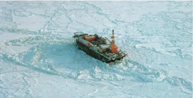
Canmar owned and operated the SSDC. This structure was a converted super tanker that had undergone extensive modifications to adapt it for use as a support structure for year-round exploratory drilling in the Beaufort Sea (Figure 13). The structure is 162 m long, 53 m wide, and 25 m high. All sides are vertical at the waterline. It was initially designed to rest in a water depth of 9 m. From 1982 to 1984, the SSDC was installed in the Canadian Beaufort Sea at the Uviluk and Kogyuk sites, where it rested on a submerged berm. In August 1986, the SSDC was modified in preparation for installations in the U.S. Beaufort Sea (1986-1988). Modification of the SSDC involved mating the drilling vessel to a semi-submersible steel base, the “MAT” (Figure 14). This steel base alleviated the need for a dredged berm, and gave it the capability to operate year-round in water depths of 7 to 24 m, and a wide variety of soil conditions. The SSDC was deployed with the MAT at the Phoenix, Aurora, Fireweed and Cabot sites in the US. Beaufort Sea. A sketch of the SSDC and MAT is shown in Figure 15.

Figure 13: SSDC at the Kogyuk site in the Beaufort Sea. Note the sprayed ice rubble surrounding the structure.

(28)

Figure 14: Artist's cut-away illustration of the SSDC and the MAT. 4.2 SSDC Instrumentation and Ice Loads

The instrumentation was different at each of the drilling sites. The following discussion describes the instrumentation at four of the six installation sites in the Beaufort Sea (no information was available for the Fireweed and Cabot sites). Note that first two sites were in the Canadian Beaufort, whereas the later two sites were in the American Beaufort. The only sites that had reliable ice load measurements were the Alaskan sites (Phoenix and Aurora). 162 m 110 m 25 m 53 m MAT (162 m x 110 m x 13.5 m)

(29)

4.2.1 Uviluk Site, 1982 – 83

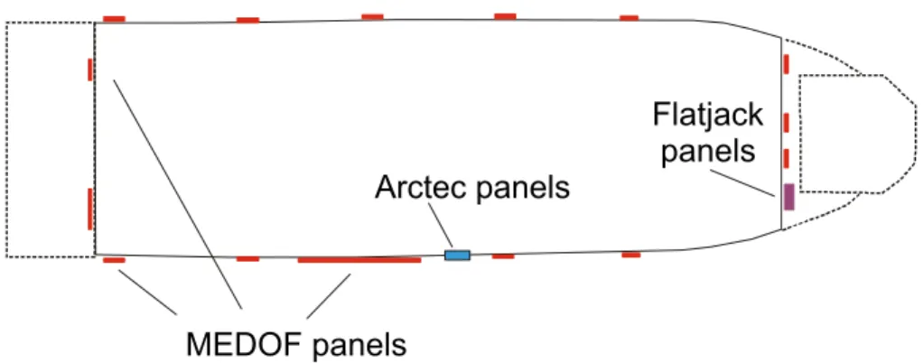
During the summer of 1982, the SSDC was deployed in a water depth of 31 m on a sub-sea berm at the Uviluk P-66 location in the Beaufort Sea. At this site, the hull was instrumented with three types of load panels: MEDOF panels, Arctec pressure panels and Weir Jones fluid filled panels (see Figure 16). The MEDOF panels (1 m x 2 m) were welded in pairs (at waterline) on all sides of the hull. The Arctec shear bar panels were arranged in a vertical array near the starboard midship. A total of 13 discrete panels with sensor areas 0.5 m x 0.5 m, 1 m x 1 m and 1 m x 2 m were welded to the vessel at this location. A total of 8 Weir Jones panels were located at the waterline on the bow of the SSDC. These units contained rectangular flatjacks (4.1 m x 2.0 m) filled with hydraulic fluid. MEDOF panels were also installed in-situ at the outer edge of the ice-berm.

A grounded rubble pile surrounded the SSDC at the Uviluk site (Figure 13) so there was no direct ice-structure interaction except during the early part of the season.

At the Uviluk site, the threshold for the instrumentation was set high in anticipation of high ice loads. However, the formation of the grounded rubble field effectively shielded the structure and the applied ice loads were below the detectable limit of the instrumentation. As a result, there are no time-series traces for the three interactions with level first year ice that occurred at Uviluk so there are no recorded ice load events from this site.

Arctec panels

Flatjack panels

MEDOF panels

Figure 16: Location of the load measuring sensors on the SSDC at the Uviluk site.

4.2.2 Kogyuk Site, 1983 – 84

During the 1983-84 season, CANMAR operated the SSDC for Gulf Canada Resources Ltd. to drill an exploratory well at the Kogyuk N-67 site, in a water depth of 28 m. The SSDC was set-down on a submarine berm that was reduced in size from the original design specifications (Hewitt et al., 1985). The three types of ice load panels installed on the SSDC while it was deployed at Uviluk (see Figure 16) were functioning at the Kogyuk site. However, at the Kogyuk site, no in-situ MEDOF panels were installed in

(30)

the surrounding ice. Hull gap LVDTs, ice pad sensors and ice reflectors (for monitoring ice movement) were positioned at specified locations in the ice.

Similar to the Uviluk site, a grounded rubble field effectively shielded the structure at the Kogyuk site.

The SSDC experienced 11 interactions at the Kogyuk site involving first year, second year and multiyear ice (Canmar, 1985). No load-time series are available for those 11 reported interactions. The most notable events were two impact events that occurred on September 25, 1983 and at break up, in June 1984 (Hewitt, personal communication). The September 25 Event occurred shortly after set down of the SSDC, while the effective ballast was estimated to be only 300 MN. A large multiyear ice floe impacted the port bow of the SSDC. The floe diameter was estimated to be 1.7 km, and the ice thickness was estimated as 3 to 4 m. The speed of the impact was estimated to be 0.25 m/s. The ice floe penetrated about eight meters, failed in pure crushing (without splitting or bending) and came to a halt. Although the impact was clearly felt, no damage or movement of the SSDC was detected. The SSDC resistance at the time of impact was estimated to be about 175 MN (Hewitt et al., 1985). Based upon this estimate and estimates of the floe mass and deceleration, Canmar estimated that the load was less than 100 MN (Hewitt, personal communication).

On June 25, 1984, a second-year floe impacted the stern of the SSDC at an estimated speed of 0.45 m/s. The floe size was estimated to be 24 by 13 km with a thickness of 1.5 to 2 m. A grounded ice rubble feature at the stern may have shielded the hull from direct contact during most of the event. The MEDOF panels registered a response to this impact, from which a load of less than 100 MN was estimated (Hewitt, personal communication).

4.2.3 Phoenix Site, 1986 – 87

In September 1986, the SSDC/MAT was deployed at the Phoenix site in Harrison Bay, Alaska, at a water depth of 17.5 m. Since the waterline was 4 m above the top of the MAT, direct ice interactions with the flat sides of the SSDC occurred.

The ice load panels installed on the hull of the SSDC while deployed at Uviluk and Kogyuk were not functioning at the Phoenix site. Instead, load panels were placed in the ice and used to monitor the ice loads. In early March 1987 four IDEAL ice force panels (0.5 m by 2.0 m) were installed in the rubbled ice surrounding the SSDC on the north side, and six additional load panels were located in the level first year ice, as shown in Figure 17. Ice loads were measured continuously from installation of the panels in March to their removal in June, 1987. In addition, the ice conditions at Phoenix were monitored via ice movement reflectors, crack displacement stations and thermistor strings. Information about the ice was also provided by aerial photography, ice rubble profiles, ice thickness, ice salinity measurements and ice observations (Blanchet and Keinonen, 1988).

(31)

N

50 m Rubbled Ice

Grounded Ice Level First-year Ice

SSDC

IDEAL Panels

Figure 17: Location of instrumentation in the ice surrounding the SSDC/MAT at the Phoenix site (1986-87).

The load panels were scanned at a rate of 20 Hz. The data were stored in a temporary buffer and the 1.5-minute average of each panel was subsequently computed. These averages were stored in a daily buffer that was recorded onto a daily disk every 24 hours. The analysis of the SSDC and its applied loads were derived from a 1.5 minute average of the panel results. Blanchet and Keinonen (1988) calculated the total load on each side of the SSDC using p SSDC scale thick incl Ideal SSDC w W x C x C x C x L L = (1) where

LSSDC = hourly average of load on impacted face

LIdeal = maximum hourly average ice load measured by the affected panel

Cincl = inclusion/cross-sensitivity coefficient

Cthick = through thickness coefficient

Cscale = scale coefficient

WSSDC = width of impacted face 162 m - starboard

52 m - stern 38 m - bow wp = 0.5 m panel width

(32)

The coefficient, Cincl, was introduced to account for the inclusion and cross sensitivity

effects associated with the load panels2. Cross sensitivity effects, which result from the simultaneous application of lateral and normal loads to the panel, can also produce increased estimates of the applied load. The combined effects of inclusion and cross-sensitivity during creep can account for an increase in load that can be represented by a load ratio of about 1.25, or Cincl of 0.8 (Blanchet and Keinonen, 1988).

The Cthick coefficient was introduced to take into account the completeness of load

measurement of the 2 m long panel measuring the applied load throughout the full thickness of the ice. Since the ice thickness differs according to the particular Event, Cthick

also varies.

The Cscale coefficient was introduced to account for any “scale effects” during an

ice-structure interaction. During creep loading, it was assumed that there was no scale effect. Hence, Cscale, was taken to be unity in the calculation of the load (Blanchet and Keinonen,

1988).

While the SSDC was at Phoenix, the landfast ice became unstable on January 30 and moved about 500 m from the northeast, creating grounded ice rubble (Figure 18). This rubble field remained stable for the rest of the winter (Blanchet and Keinonen, 1988). After the formation of the port side ice rubble on January 31, the ice around the SSDC/MAT became immobile. The 500-m long wake refroze on the starboard side and beyond the stern rubble. Although periods of high winds occurred before break-up, no significant movements of the landfast ice were measured. The landfast ice did experience a cyclical motion due to wind, thermal or tidal stresses. The decay of the rubble began at the end of May. The surface of the ice melted at low areas within the rubble and the level ice. Water accumulated on top of the ice until it was able to drain through holes in the ice. There were six notable ice-structure interaction events between March and June, 1987. Each of the interactions occurred when the surrounding landfast, rubbled ice encroached upon the port side of the SSDC, due to thermal and wind-driven stresses. Global loads were derived from the response of the four load panels along the port side of the SSDC (see Figure 17). The global load associated with those six interactions ranged from 25 Mn to 74 MN.

2

Studies have shown that the stress field in the ice is disturbed when objects are introduced in to the ice (see e.g. Croasdale and Frederking 1986). As a result, the response registered by the load panels can be different than stresses measured in ice. This artifact of the load panels is produced by the difference in stiffness between the load panel and the surrounding ice. The load panel affects the local stress distribution in the ice and introduces a ‘hard spot’.

(33)

Figure 18: Photograph of the SSDC at the Phoenix site. Note the large rubble field surrounding the structure.

4.2.4 Aurora Site, 1987 - 88

In 1988, the SSDC/MAT was deployed at the Aurora site in a water depth of 21 m. At this site, ten in-situ load panels monitored the applied load adjacent to the hull of the SSDC as well as the load applied in the region outside the rubble ice (Figure 19). Five of the panels were located in the rubble off the bow. Two other panels were installed at starboard, and three panels were installed in rubble near the stern. Due to the large amount of broken ice and the instability of the ice to the north of the SSDC, no in-situ ice load panels were installed on the port side of the SSDC. Ice conditions surrounding the SSDC were monitored through crack displacement stations, thermistor strings, ice movement reflectors, wire line devices. Numerous boreholes were used to measure ice thickness and determine the profile of the underside of the rubble (Blanchet and Wiefelspuett, 1988).

Ice conditions at the Aurora site were more dynamic than at the other sites. The SSDC was bounded on the south by landfast ice that had stabilized by the end of November, 1987. The ice to the north, east and west of the SSDC was more mobile. Borehole drilling indicated that the rubble in all sectors was floating. Rubble formations near the bow stern and starboard stern corners had sail heights that ranged from 2 to 3 m, with individual blocks up to 4 m high. The enclosed flat pans consisted of single or rafted layers of level ice. The ice in contact with the starboard side of the SSDC was mainly level ice, with isolated rafted areas and some rubble that extended less than 1 m from the hull.

(34)

50 m N

Landfast Ice

Rubble

Level Ice - Mobile

panel used in load calculation for Events involving the bow

panel used in load calculation

for Events involving the starboard, stern Port Side

Starboard Side

Figure 19: Location of instrumentation in the ice surrounding the SSDC/MAT at the Aurora site (1987-88).

During the project period, the average level ice thickness surrounding the SSDC increased from 1.22 m to 1.55 m, with a maximum of 1.58 m on June 1, 1988. The growth of the consolidated layers at both the bow and stern locations were estimated to be from 2.2 m in March to 3.5 m in June for the bow ice, and from 1.7 m in March to 3.0 m in June for the stern ice.

Ice adjacent to the SSDC developed cracks that extended 45° from the centerline of the SSDC, and divided the surrounding ice into four regions classified as the bow, starboard, stern and port sectors (Figure 19). Ice at the bow, stern and port side of the structure moved with the predominant wind direction, which was generally in the east-west direction3. Ice in the port sector remained unstable throughout winter until breakup, with daily movement from 0 to 20 m. The ice sheet in the starboard section had a cyclical motion between the shoreline and structure (normal to the longitudinal axis) that was wind and temperature driven.

The ice loads at the Aurora site were determined using the same methodology as that at the Phoenix site. Nine loading events occurred between March and June, 1988, seven of

3

The ice movement direction was consistently 30° to 60° to the right of the wind direction. At Aurora, 54% of winds were from the ENE direction and 30% of the winds were from WSW direction. All winds greater than 16 m/s were from E or ENE for all but one day (February 21, 1988).

(35)

which were analyzed. These events resulted from wind/thermally driven stresses and involved the bow and starboard sides of the vessel. Load estimates for interactions involving the bow were obtained from the in-situ load panel located towards the centre of the bow. The two surrounding panels on the bow were damaged during the second ice-bow interaction of that season. Global load estimates for the event that involved the starboard side of the vessel were obtained from the in-situ panel located on the starboard side, near the stern. The load occurrences at Aurora were classified as pure creep interactions, or a combined failure mode of creep and “racheting”.

4.2.5 Overview of Ice Loads on the SSDC

Figure 20 shows a plot of the Line Load as a function of the ice thickness for all of the events in which load information was available (Phoenix and Aurora sites). Note that for all of these events, a rubble field surrounded the SSDC. The data in the plot have been subdivided according to the state of the rubble surrounding the SSDC. Although the rubble fields were mostly floating, there were grounded regions close to the SSDC at the Phoenix site.

SSDC/MAT

0.0 0.5 1.0 1.5 2.0 2.5 3.0 0.0 0.5 1.0 1.5 2.0 2.5 3.0 Ice Thickness (m) Line Load (MN/m) Floating Rubble Floating & Grounded Rubble

First-year Level Ice

(36)

5.0 CAISSON-RETAINED ISLAND (CRI)

5.1 Description of the CRI

Esso Resources Canada Ltd. originally built this structure, but it is now owned by Arctic Transportation Ltd. It was developed as a means of reducing dredge quantities, as compared to the more traditional sand island. The CRI was built in 1982-83 and first deployed in the Canadian Beaufort Sea in the summer of 1983. The design has 8 individual caissons (43 m long x 12.2 m high x 13.1 m wide) in a ring (see Figure 21). Two pre-stressed bands of steel wire cable hold the caissons together. The central core, which is 92 m across, is filled with sand to provide a surface for drilling operations and to provide stability against applied loads. The CRI is an 8-segment octagonal-shaped steel structure about 118 m across on the flats, 12 m high and the outer face is inclined (30° from the vertical).

4 9 .2 m 1 1 8 .8 m 4.6 m 12.3 m -9 m Sea Floor Caisson

Figure 21: Illustration of the Caisson Retained Island (after Croasdale, 1985)

The CRI was deployed for three seasons in the Canadian Beaufort Sea:

1. From September 1983 to April 1984 it was deployed at the Kadluk O-07 in Mackenzie Bay site at a water depth of 14.5 m. A spray ice island was constructed to the north of the CRI to provide an emergency relief well drill site.

2. In August 1984 the CRI was moved to the Amerk O-09 site where it remained until March 1985.

3. From October 1986 to January 1987, the CRI was deployed at the Kaubvik I-43 site.

5.2 Hull Instrumentation on the CRI

Instrumentation on the CRI consisted of sensors for ice loads on the outer surface of the caisson, strain gauges on structural elements of the caisson and geotechnical sensors in the sand core and under the foundation (Hawkins et al., 1983). A schematic of the layout

(37)

of the sensors is shown in Figure 22. The majority of the load sensors were installed on the north, northeast and northwest caissons, to provide coverage to the faces over the anticipated, predominant direction of ice movement. Ice force sensors on the outer surface comprised three different sizes and types:

1. The microcells, which had a diameter of 165 mm, were the smallest sensor. They were a temperature-compensated, strain-gauged diaphragm-type of sensor. Four clusters of 4 sensors were flush-mounted on the north quadrant of the caisson at the waterline, and several more pairs were mounted on the adjacent faces (Figure 22). They measured point (or local) ice loads and had a high load capacity of 35 MPa and a short response time.

2. The maxicell, which had a diameter of 815 mm, was a sensor that measured pressure in a spiral coiled hydraulic tube sandwiched between two steel plates. It was, effectively, a load cell with an equivalent capacity of 7 MPa. Because of its construction it did not have a short response time. A total of 8 of these sensors were mounted on the southern half of the caisson. They were supported by structural stringers and were flush with the surface. During their first year of operation, the maxicells proved to be unreliable. They were subsequently replaced by a pair of microcells, which were mounted on an adapter plate (Croasdale et al., 1988).

3. The third type of sensor was a shear bar-type with a load sensing surface 2.1 m high by 0.5 m wide. Strain gauged shear bars sensed the normal component of the ice load applied to them. They had a full-scale range of about 3 MPa. Nine of these sensors were deployed around the northern half of the caisson.

The internal structure of the caissons was also instrumented with 156 weldable strain gauges. The locations were determined from a finite element analysis that also provided a means for interpreting ice loads from the measured strains. Geotechnical sensors were used to measure the response between the caisson and the sand and foundation. This instrumentation included total pressure cells, pore pressure cells and inclinometers. The instrumentation was sampled at a frequency of either 0.1 Hz or 1 Hz. To reduce the quantity of stored data, real-time data processing techniques were used. This involved storing the average, variance and peak reading for each sensor over a five-minute interval.

(38)

shear bar microcells

N

25 m

Figure 22: Illustration of the location of the instrumentation on the hull of the CRI.

5.3 Field Instrumentation and Ice Loads on the CRI

In addition to the hull instrumentation, a number of different sensors were placed in the ice surrounding the CRI. In the following sections the ice conditions, field instrumentation, and measured loads are described for each of the three sites.

5.3.1 Kadluk, 1983-84

When the CRI was deployed at Kadluk in 1983-84, early ice movement was restricted by grounded second-year ice, and an ice rubble field did not form. A later movement of the landfast ice allowed ice about 1.0 m thick to interact, directly, with the caissons. By the first week of March, the surrounding first year sea ice was about 1.7 m thick, and there was an extensive grounded rubble field on the southwest side of the CRI. A few small grounded multiyear floes were observed to the east and north of the CRI (Johnson et al., 1985). On March 11, strong southerly winds caused ice on the north side of the CRI to break away and move out to sea, which left the CRI-ice island-rubble area as a peninsula on the edge of the inshore flat ice.

(39)

During the spring of 1984, 18 cylindrical, biaxial ice stress sensors4 were installed in the level ice south of the CRI, beyond the rubble (Cox, 1987). Due to complications, the in-situ sensors were not finally positioned until the first week of April. Since ice north of the CRI remained thin and continued to move offshore at that time, the sensors were deployed at six sites south of the island (on the shoreward side, Figure 23). At each of the six sites, the sensors were located at ice depths 0.3 m, 0.8 m and 1.3 m. An Exxon pressure panel was installed on the south side of the structure, about 20 m from Site 2, with the panel facing 6° from north. In addition, the ice temperature, ice movement and wind speed and direction were monitored.

CRI - Kadluk Shear ridge Ice rubble Ice rubble extent Site 1 Site 4 Site 2 Site 5 Site 6 Site 3 Exxon panel 50 m x x x x x x x x x x x xx x x x x x x x x x x x x x x x x x x x x x x x x x x x x x x x x xx x x x Small ice ridge Open water N

Figure 23: Ice conditions and instrumentation at Kadluk, spring 1984 (after Johnson et al., 1985 with adaptations).

4

The biaxial stress sensor consists of a stiff, steel cylinder that allows the principal ice stresses normal to the axis of the gauge to be determined by measuring the radial deformation of the cylinder in three directions (using vibrating wire technology). The sensor itself is 20.3 cm long, 5.7 cm in diameter and has a wall thickness of 1.6 cm. The biaxial stress sensors have been used to measure thermal stresses in New Hampshire lakes (Cox, 1984) and ice forces on Adams Island (Frederking et al., 1984).

(40)

Johnson et al. (1985) noted that when the ice was not subjected to any appreciable load, the principle stress direction varied with depth. However, when the panel stress exceeded 100 kPa, the principle stress directions became aligned in the top, middle and bottom of the ice sheet. Stresses at all depths had a diurnal variation in response to air and ice temperatures. The complexity of the ice stress distribution versus depth was attributed to the occurrence of bending failure of the level ice (observed along the length of the rubble pile in front of the structure), with contributions from thermal stresses in the ice sheet. Lateral variations in the stress at any given level were also complex. However, in general, the average full thickness ice stress did appear to increase from west to east along the measurement line. This was attributed to the presence of grounded multiyear ice at the east end of the line of the sensors (Johnson et al., 1985). During inactive periods the ice did not show the lateral increase in stress from west to east.

No time-series traces are available for the global load on the CRI at Kadluk. However, Johnson et al. (1985) computed the total load from the average normal and shear stress measurements at Sites 1, 2, 3 and 4 and summing them across the ice peninsula. They state that the total ice load on the CRI-rubble complex at Kadluk during April and May was thermally induced. The peak structural load associated with the thermal activity of the ice was estimated to be about 150 MN. In their analysis, Johnson et al. (1985) did not account for the influence of ice rubble on the magnitude of structural loads.

5.3.2 Amerk, 1984-85

In 1984-85 the CRI was located at Amerk, where it was surrounded by grounded rubble (Figure 24). As such, the grounded rubble transmitted ice loads to the underwater berm and the caissons experienced negligible load (Croasdale, 1985). In general, the rubble had a sail height from 0 to 4 m above sea level, although the northeast part of the rubble field had sails that approached 10 m in height (Sayed et al., 1986).

In March 1985, in-situ ice sensors were installed in the rubbled ice surrounding the CRI. Since the floating ice was expected to move in a predominantly westward direction and thermal stresses/expansion would be applied relative to the nearest shoreline, the east and south sectors of the rubble field were monitored for ice pressure and movement (Sayed et al., 1986). Various types of instrumentation were installed in the rubbled ice, including two Exxon Production Research (EPR) panels, three HEXPACK panels, an Ideal panel and a biaxial Canada Marine Engineering sensor (CMEL-IV) (Figure 25). The in-situ instruments were recorded at five-minute intervals. Ice movement records supplemented this information. The ice displacement was determined from a system of survey reflectors that were used in conjunction with an electronic distance measuring (EDM) instrument and a theodolite. Wind and temperature data also were recorded at the site.

(41)

Figure 24: Ice rubble surrounding the CRI at the Amerk site. N IDEAL panel Exxon panels HEXPACK sensors 50 m CMEL IV sensor

Limit of ice rubble CRI - Amerk

Panel 7

(42)

When the CRI was deployed at Amerk, over the winter of 1985-86, only the Exxon panel along the southern edge of the rubble (panel 7 in Figure 25) yielded appreciable results. All other sensors installed in the ice around the CRI showed no response. The stress-time trace for panel 7 is presented in Figure 26. During the period of instrumentation (March to May), the panel showed heightened activity during April 1 to 7, and then again beginning on April 22, 1985. During that period, the thickness of the refrozen rubble layer was 2.5 m. Sayed et al. (1986) estimated the load per unit length to be 500 kN/m, assuming the stresses were uniform across the frozen rubble. Since negligible stresses were measured near the caisson, it was concluded that the presence of grounded rubble resulted in significant attenuation of the applied load at Amerk (Sayed et al., 1986).

0 50 100 150 200 250 85 90 95 100 105 110 115 120 Julian Day

Exxon panel stress (kPa)

26-Mar 30-Apr

CRI Amerk 1985 - panel 7

Figure 26: Stress measured on Panel 7 at the Amerk site from Julian Day 85 (March 26) to Julian Day 120 (April 30), 1985 (after Sayed et al., 1986 with adaptations)

5.3.3 Kaubvik, 1986-87

During the winter of 1986-87, the CRI was at the Kaubvik site. Moving pack ice surrounded it, and thin first year ice acted directly upon the caissons. In January, rubble began to develop around the structure. By February, a grounded rubble field surrounded the caisson, and remained stable until May (Figure 27). The thickness of the consolidated layer in most areas was about 2.5 m (below water level), and it was slightly thicker under rubble sails (Frederking and Sayed, 1988).

(43)

Figure 27: Photograph of the grounded rubble field around the CRI at the Kaubvik site.

A joint measurement program was carried out at the Kaubvik site with participation from Esso Resources Ltd, Memorial University of Newfoundland and the National Research Council of Canada (Croasdale et al., 1988). Esso Resources measured and recorded ice pressures on the caissons of the CRI and monitored the geotechnical behaviour of the foundation. Memorial University determined the strength and strain characteristics of the ice rubble and measured ice pressures and strains in the level ice surrounding the grounded rubble. The NRC measured the internal ice pressures, and the movements and profiles of the grounded rubble.

Four types of stress sensors were used to monitor the in-situ pressures in the ice rubble. The sensors were placed along radial lines extending away from the CRI, in order to measure the lateral stress profile of the load transmitted through the rubble field (see Figure 28). Three Exxon panels were oriented south-east of the caisson, extending to the outer edge of the rubble, where they would experience the effect of thermal expansion of the ice.

(44)

IDEAL panels Exxon panels Exxon panels HEXPACK sensors N 50 m CRI - Kaubvik 1 2 3 4 1 3 2 1 5 6 1 2 3 Open Water

First Year Pack Ice

Ice rubble on 5 January

First Year Pack Ice Open Water

Grounded rubble on 4 Jan

Figure 28: Location of the in-situ stress sensors in the rubble field surrounding the CRI at the Kaubvik site.

Since most storms approached from the northwest, the ice shear zone would be driven towards the CRI from this direction. Therefore, the majority of in-situ load panels were installed northwest of the CRI. The instrumentation included a radial line of four Exxon panels (0.5 m x 2 m), a rosette of three 1 m x 1 m IDEAL panels, a 1 m x 2 m panel and a rosette of circular HEXPACK panels (0.46 m diameter). The Exxon panels, IDEAL panels and HEXPACK panels were scanned and recorded at respectively 10, 15 and 30 minute intervals.

Ice movement was determined from an array of prism reflectors used in conjunction with an electronic distance measuring (EDM) instrument and a theodolite. Rubble surface profiles were taken along approximately radial lines from the CRI.

Memorial University installed three rosettes of BP-type sensors (mercury-filled, 75 mm diameter) in March, 1987 to monitor the late winter in-situ ice pressures associated with the level ice. By March, growth of the rubble field had stabilized. Therefore, the BP-type sensors were installed in the level, landfast ice, about 50 m southeast of the grounded rubble, at a depth of 0.6 m (Marshall, 1990, see Figure 29). The rosettes were arranged

(45)

so that one sensor in each rosette recorded the stress towards a given survey point on the southeast caisson of the CRI. The data were scanned and recorded every 2 minutes.

IDEAL panels Exxon panels Exxon panels Three rosettes of BP-type sensors HEXPACK sensors N 50 m CRI - Kaubvik 1 2 3 4 1 3 2 1 5 6 1 2 3 Rubble on 6 January Rubble on 7 January Rubble on 12 January Late winter rubble extent Landfast, level first year ice

Figure 29: Late winter map of rubble extent around the CRI-Kaubvik showing location of BP-type sensors (after Frederking and Sayed, 1988; Marshall, 1990; with adaptations).

During the early winter period of 1987, the CRI at Kaubvik was directly exposed to advancing ice. However, the hull-mounted sensors showed that the early winter ice-structure interactions generated low ice forces, typically global loads of the order of 10 MN (Croasdale et al., 1988).

As the winter progressed, an extensive rubble field developed around the CRI at Kaubvik. The ice load panels that were installed in the rubble measured the in-situ ice stress (Figure 30). During the January 1987 field trip to Kaubvik, field personnel noted the occurrence of two rubble building events, one on the east side on the evening of January 5, and the other on the north-west side on the evening of January 7. The load panels registered a response to the January 7 event, at which time the rubble extent was in the vicinity of Exxon panels 3 and 4. Exxon panels 1 and 4 showed that the stress increased over a period of 2.5 hours, whereas Exxon panel 2 increased only slightly and