Calculation of interface tension and stiffness in a two dimensional Ising Model by Monte Carlo simulation

Calculation of Interface Tension and Stiffness in a

Two Dimensional Ising Model by Monte Carlo

Simulation

by

Isaac Samuel Chappell II

Submitted to the Department of Physics

in partial fulfillment of the requirements for the degree of

Master of Science

at the

MASSACHUSETTS INSTITUTE OF TECHNOLOGY

September 1998

©

Isaac Samuel Chappell II, MCMXCVIII. All rights reserved.

The author hereby grants to MIT permission to reproduce and

distribute publicly paper and electronic copies of this thesis

document in whole or in part.

Author

... .... .. ...

....

Department

of

Physics

August 7, 1998

Certified by

...

4e-Jens

Wiese

Professor

Thesis Supervisor

Accepted by...

A',C , - ,UC sT;UM . / Tho s J. Greytak

O:

T0t4OLO Y

Associate Department Hea6 for Education

Calculation of Interface Tension and Stiffness in a Two

Dimensional Ising Model by Monte Carlo Simulation

by

Isaac Samuel Chappell II

Submitted to the Department of Physics on August 7, 1998, in partial fulfillment of the

requirements for the degree of Master of Science

Abstract

The two dimensional Ising Model is important because it describes various condensed matter systems. At low temperatures, spontaneous symmetry breaking occurs such that two coexisting phases are separated by interfaces. These interfaces can be de-scribed as vibrating strings and are characterized by their tension and stiffness. Then the partition function can be calculated as a function of the magnetization with the interface tension and stiffness as parameters.

Simulating the two dimensional Ising Model on square lattices of various sizes, the partition function is determined in order to extract the interface tension. The configurations being studied have low probability of actual occurrence and would re-quire a large number of Monte Carlo steps before obtaining a good sampling. By using improved estimators and a trial distribution, fewer steps are needed. Improved estimators decrease the number of steps to achieve a certain level of accuracy. The trial distribution allows increased statistics once the general shape of the probability distribution is calculated from a Monte Carlo simulation. For small lattice sizes, it is easy to run Monte Carlo simulations to generate the trial distribution. At larger lat-tice sizes, it is necessary to build the trial distribution from a combination of a Monte Carlo simulation and an Ansatz from theory due to lower statistics. The extracted values of the interface tension agree with the analytical solution by Onsager.

Thesis Supervisor: Uwe-Jens Wiese Title: Professor

Acknowledgments

To Bootz and Houndini:

to know them is to love them, and to love them is to know them. those who know them, love them,

Contents

1 Introduction 8

1.1 Ising Model ... ... . 9

1.2 Monte Carlo Methods ... ... . 10

2 The Ising Model 12 2.1 Properties of the Ising model . ... .... 12

2.1.1 D efinitions . . . 12

2.1.2 Phase Transition and Spontaneous Symmetry Breaking . . . . 14

2.1.3 Interface Tension and Stiffness . ... 14

2.2 Theory and Re-weighting . ... ... 15

2.2.1 Interfaces as Vibrating Strings . ... 15

2.2.2 Re-weighting: Theory ... 16

3 Monte Carlo 18 3.1 Monte Carlo ... ... 18

3.1.1 Markov Chains ... ... 19

3.1.2 Ergodicity and Detailed Balance . ... 19

3.2 Metropolis algorithm ... ... 20

3.3 Cluster Algorithm ... ... 21

3.3.1 Improved Estimator : (M2) ... .. 23

3.4 The Monte Carlo methods used . ... .. 24

4 Implementation and Results 28

4.1 Implementation ... ... ... 28

4.1.1 One Dimensional Ising Model ... 28

4.1.2 Two Dimensional Ising Model . ... 29

4.2 Results ... .... ... ... ... 30

4.2.1 Statistical Errors: Monte Carlo . ... 31

4.2.2 Statistical Errors: General ... . 31

4.2.3 System atic Errors ... ... 32

5 Conclusion 33

A Figures 35

List of Figures

A-1 Two regions of different spins separated by two interfaces ... 36

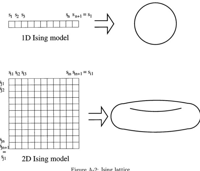
A-2 Ising lattice ... ... .. ... 37

A-3 One phase configuration ... ... 38

A-4 Two phase configuration ... ... .. 39

A-5 Two possible two phase configurations with the same free energy . . . 40

A-6 Original magnetization-dependent partition function, Z(M) .... . 41

A-7 Effective magnetization-dependent partition function, Zeff(M) . . . . 42

A-8 Effect of the improved estimator: with improved estimator ... 43

A-9 Effect of the improved estimator: without improved estimator . . . . 44

A-10 magnetization-dependent partition function for f = 0.47, L = 8 . . . 45

A-11 magnetization-dependent partition function for

f

= 0.47, L = 12 .. 46

A-12 The surface tension for3 = T ... ... . 47

A-13 The surface tension for/3 = 0.47 ... ... . . . . 48

List of Tables

B.1 Magnetization (M) and susceptibility X data from D = 1, L = 4

Cluster algorithm ... ... 51

B.2 Surface tension a, magnetization (M), and susceptibility x for D=2, = Tc ... ... ... ... ... .. ... 52

B.3 Surface tension a, magnetization (M), and susceptibility X for D=2, / = 0.47 ... . ... 53 B.4 Surface tension a, magnetization (M), and susceptibility X for D=2,

Chapter 1

Introduction

The Ising model is one of the best understood statistical physics models not only because of its application to a variety of physical systems but also for its ability to be solved in one and two dimensions. It can be applied to a number of systems which have a phase transition. The Ising model describes a particular class of systems in terms of spins that can be "up" or "down" located on a lattice. There is a phase transition in this type of system between disordered spin configurations and configurations where groups of neighboring spins are parallel. In this configuration, both "up" and "down" groups occur and are separated by interfaces. There exist configurations called two phase configurations in which both "up" and "down" groups occur in large groups and these are interesting to study.

Many systems are higher dimensional in nature and methods need to be developed to describe and understand such physical systems. Using a Monte Carlo method of computer simulation, in which random numbers are used to simulate different states, the Ising model can be studied. A method for gaining information about higher dimensions has been developed and to test this method a test case of the solvable

examples of one and two dimensions must be checked. Specific observables of a

particular class of configurations are calculated and compared to their analytical results.

Chapter Two summarizes general features of the Ising model pertinent to the research. It also presents a theory of the two phase configurations which exists in the

two dimensional Ising model and is a key focus of the research. Some of these results are used to calculate the observables of the model. Also, the concept of re-weighting is explained to show how data is collected.

Chapter Three focuses on the Monte Carlo methods used to calculate observables and to generate configurations of the system. The Metropolis and Cluster methods and their application to this research are discussed.

Chapter Four contains the actual application of the numerical method to the Ising model and the results of the calculation. This method is tested by comparison with the analytical solutions.

Chapter Five contains the conclusion and discusses the usefulness of this approach to higher dimensional Ising models.

1.1

Ising Model

The Ising model is formulated in terms of spins on a quadratic lattice. The spins can either be "up" or "down". It this research, we use periodic boundary conditions.

The Ising model is characteristic for several physical systems which all have a phase transition. At this phase transition, characteristics of the set of configurations change by being below a certain temperature, called the critical temperature T,. The most common example is water turning into ice below the freezing point.

The phase transition in the Ising model is characterized as second order, meaning it is a smooth transition from one configuration to the other. It is seen as a change from a more or less random collection of spins to configurations where larger islands of parallel spins are present. Although absent in one dimensional models, this phase transition exists and is very important in higher dimensional models. However, it is not very well understood in higher dimensions because of a lack of an exact solution except in two dimensions where an exact solution was found by Onsager [1].

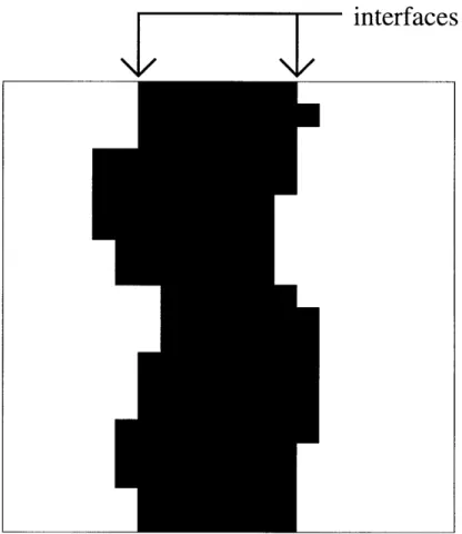
A particular set of configurations in the class of ordered configurations that exist below the critical temperature is the one where two regions of different spin coex-ist, separated by interfaces (Fig. A-1). With periodic boundary conditions in two

dimensions, there are two interfaces and the two phase configurations requires a large amount of free energy. The free energy can be parameterized by the interface tension and stiffness, two characteristics that describe the interface. The interface tension measures the free energy per unit length of the interface. The stiffness determines how much energy is used by the curvature of the interface. These are the properties that are being studied in this research.

1.2

Monte Carlo Methods

To study these characteristics, the particular two phase configurations must be gen-erated. To generate these configurations, a Monte Carlo method is used. Monte Carlo methods involve using random numbers to generate configurations. From the configurations generated, measurements of the characteristics called observables can be made and averaged over to give a thermal average value of the observable, usually calculated from a partition function. A partition function is a description of all the configurations of the system with a statistical weight based on an exponential of the configuration's energy. By Monte Carlo methods, the same set of observable are cal-culated from the model's Hamilton function, a function which describes the energy of a configuration.

However a problem arises. The two phase configurations have a high energy and therefore low probability and rarely occur. Normal Monte Carlo methods can generate such configurations by "importance sampling," which generates configurations based of their probability as they weigh in the partition function. The idea of "re-weighting" the partition function is used to create a new effective partition function that has the same configurations but with probabilities that favor the two phase system and allow their more frequent generation through Monte Carlo methods.

To further increase the efficiency of the method, both Metropolis and Cluster algorithms were examined to determine the best one for the method. The Metropolis algorithm was first used in the one dimensional example but it was found inefficient for this research. The Cluster algorithm, specifically the Swendsen and Wang cluster

algorithm [2], was then used and found to work well in one and subsequently two dimensions. Another method to increase the efficiency was the use of "improved estimators," routines that improved the efficiency of each Monte Carlo step.

In the end, the data gained from the computer simulation was compared to the analytical results given by Onsager [1] for one and two dimensions. Agreement with these results proved the accuracy and efficiency of this method of calculation.

Chapter 2

The Ising Model

2.1

Properties of the Ising model

2.1.1

Definitions

The general Ising Model consists of a d-dimensional lattice of length L made up of spins s. The lattice can have open or periodic boundary conditions. In this research, one- and two-dimensional Ising models with periodic boundary conditions are used. This means the lattice is bounded in all directions, with the last spin SL in one direction connecting to the first spin sl in the same direction (SL+1 = Sl). In one dimension, this forms a circle; in two dimensions, it is a torus (Fig. A-2). The spins at each lattice site take on one value of either +1 ("up") or -1 ("down"). The values

of all the spins specify a configuration, referred to as

[s].

The classical Ising Hamilton function for a configuration of spins is given as follows:

H[s] = -

S

Jssy + Bsx. (2.1)

(x,y)

where J is the coupling constant, B is the magnetic field strength, and s, and s, are the individual spins in the configuration. The (x, y) in the sum means that the sum is over all nearest neighbors on the lattice. Because of the +1/-1 values of the spins,

This means that an interchange of +1 and -1 spins does not change the value of the Hamilton function. With the magnetic field nonzero, this is not true.

The partition function, Z, corresponding to this Hamilton function is a function which describes all of the possible configurations of the system mathematically:

Z = e- H []. (2.2)

[s]

The sum is over all possible configurations [s] and each configuration has a factor of

e-PH[s], called its Boltzmann factor. This factor consists of an exponential of minus the reciprocal of the absolute temperature, represented by / = 1/kT multiplied by the energy of that configuration, given by the Ising Hamilton function, Eq. (2.1).

An observable, 0, can be evaluated for each individual configuration, O[s]. An example of an observable is the magnetization, M. From the partition function, thermal expectation values of observables, (0), can be calculated by

(0) = - O[s]e - H[s], (2.3)

where O is the observable being calculated. An important observable for this Ising Model is the magnetization, M:

M[s]= s. (2.4)

Another important quantity is the susceptibility,

x = ((M2) - (M) 2) (2.5) The susceptibility measures the fluctuations in the magnetization and is the difference of the thermal average of the magnetization squared ((M 2) = ((EXs )2)) and the square of the thermal average of the magnetization ((M)2).

2.1.2

Phase Transition and Spontaneous Symmetry

Break-ing

There exists a certain temperature below which areas of parallel spins, called domains, start forming without a magnetic field present. This temperature is the critical tem-perature, Tc, and has been calculated by Onsager [1]. This is also characteristic of a phase transition, a change of configurations from more or less random ones to more ordered ones. This particular phenomenon is called spontaneous symmetry breaking. The phase transition is characterized by its discontinuities. In the Ising model, the discontinuity occurs in the susceptibility while the magnetization smoothly changes with temperature. This type of phase transition is called second order.

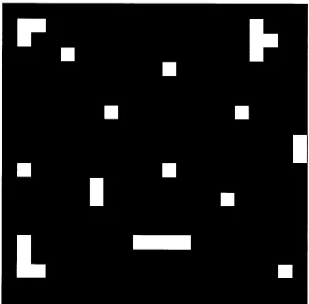
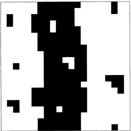
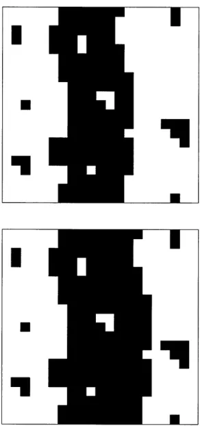
There are two main types of configurations possible in the two dimensional Ising model that characterize the spontaneous symmetry breaking. One class of configura-tions is formed by a single large domain of one particular spin configuration (Fig. A-3). This large domain may have smaller regions of the opposite spin configuration inside it. It is these configurations that are most common and highly probable. The sec-ond set of less probable configurations is formed by a band of each particular spin configuration that goes around the cyclic boundaries of the system (Fig. A-4). This configuration can also have smaller clusters of the opposite spin configuration inside each of the bands. Since it has both phases of "up" and "down" spins coexisting in the same configuration, it is called a "two phase" configuration. The phases are separated by two boundaries called interfaces.

The two phase configuration has a very low probability due to its high free energy cost of the two interfaces. The high energy implies low Boltzmann factors which exponentially suppresses these configurations.

2.1.3

Interface Tension and Stiffness

The interfaces can be characterized by their interface tension, o, which measures the free energy per unit length of the interface, F oc aL. Also useful is the interface

interface.

Onsager solved the two dimensional Ising model without a magnetic field [1]. In studying the two phase configuration, he found the interface tension for an infinite lattice was given by

1 log[1 + exp(-2PJ)

a = 2J - ~ log[ - ] " (2.6)

P 1 - exp(-20J)

The results of the numerical simulations should approach this number as the lattice size is increased.

2.2

Theory and Re-weighting

2.2.1

Interfaces as Vibrating Strings

Professor Wiese has developed a theory in two dimensions that describes the two phase configurations and a partition function based on the magnetization of such config-urations [3]. This theory describes the interfaces as vibrating strings. A Hamilton function for the strings is written down and partition function is derived as a function of the magnetization of the configuration. This partition function as a function of the magnetization has the form:

Z(M) =

~e-H[s]6M[],M.

(2.7)

[s]

By using the Kronecker delta function, only configurations with the right magneti-zation are included. The magnetimagneti-zation-dependent partition function relates to the normal definition of the partition function by

Z = E Z(M). (2.8)

The actual partition function which describes the system as a function of the magne-tization is calculated as [3]

M M

Z(M) = exp(-f L2)[D( - L2) + D( + L2) + exp(-2aL)]. (2.9)

m m 2rL

The two Gaussian distributions, D(M'/m) = V1/2rxL 2 _exp(-M'2_/2m 2_xL 2_{) with}

M' = M -mL 2, represent the configurations in which a large cluster with

magnetiza-tion ±mL2 of one particular spin configuration exists as shown in Figure (A-3). The

two phase configurations are represented by a plateau near zero magnetization, rep-resented by the third term on the right hand side. The two phase configurations have a magnetization near zero because of the existence of approximately equal numbers of +1 and -1 spins. This is because the free energy is just a function of the length of the interfaces, not the area of between them. Two configurations could have different numbers of +1 spins but the same interface shapes and thus nearly the same free energy as shown in Figure (A-5).

Also important is the ratio:

Z(0) _ x

Z(O - I) , exp(-2oL) (2.10)

Z(mL2) V 27

of the minimum and maximum values of the partition function Z. This equation

allows for the calculation of the interface tension a and interface stiffness K if the

average magnetization, susceptibility and the partition function values are known.

2.2.2

Re-weighting: Theory

To investigate the two phase configurations more closely, the idea of re-weighting the partition function is used. This means that the partition function, which assigns a probability based on energy, is re-weighted so that certain configurations, in this case the two phase configurations with high energy, are given a higher probability. As long as this re-weighting is taken out at the end, the physics described is the same as before. Careful consideration must be taken in re-weighting and this will be discussed

later in Section 3.4.1.

The way the partition function is re-weighted is based on another function called the trial distribution. The trial distribution, pt(M), is a function which has all the in-formation about how the probability should be re-weighted. A new partition function is created, based on a new Hamilton function. This new effective Hamilton function, Heff, is the original Hamilton function plus a function of the trial distribution:

Heff[S] = H[s] + log(pt(M([s]))) (2.11)

Note that the trial distribution, pt(M), is a function of the magnetization M. This results in a new effective magnetization-dependent partition function:

Zeff(M) = Z(M)/pt(M) (2.12)

The use of the trial distribution is to increase the probability of the configurations of interest, the two phase configurations. Without the trial distribution, the distri-bution of the probabilities of magnetizations favors the one phase configurations of magnetization close to (M) (Fig. A-6). The trial distribution was chosen to increase the probability of getting the two phase configurations with certain magnetizations. The total effect is that of an approximately flat effective probability distribution of the configurations, as shown in Graph (A-7).

Chapter 3

Monte Carlo

3.1

Monte Carlo

To investigate the two dimensional Ising Model, a Monte Carlo simulation is used. Monte Carlo methods have been used since the middle of the last century but were first documented as such in the 1940's as an offshoot of atomic bomb research [4]. Primarily, Monte Carlo methods entail calculating the value of something using ran-dom numbers. In this research, Monte Carlo methods were used to generate a Markov chain, or a string of configurations, from random numbers. Normally, to calculate an observable, an integration is performed over the whole configuration space of the system. Monte Carlo methods generates a thermal average using a Markov chain of configurations.

The Monte Carlo method simply models an experimental point-of-view of cal-culating observables. Experimentally, observables would be obtained by an average over several measurements taken at a physical system at some fixed temperature. The system goes through a number of different configurations possible at the fixed temperature with different values of the observables. The distribution of these val-ues gives a picture of the partition function for the system at that temperature. In the computer, a similar process is simulated: a "computational" model is set up at a temperature and possible configurations are generated through a Markov chain of configurations. In this case, the Markov chain is based on spin flips.

3.1.1

Markov Chains

A set of specific spin values at the lattice vertices is defines a configuration denoted by [s(i)]. A Markov chain is a set of configurations which map to each other: [s(i)] -4 [s(i+l)] by use of some transitional probability, W([s( i)] -+ [s(J)]). The choice for the

probability of a configuration is its Boltzmann factor: P[s(i)] = exp(-3H[s(i)]). This

choice allows for a simplification of the calculation of observables. An observable is calculated from statistical mechanics as

(0) = EO exp(-H[s]) (3.1)

with the summation being carried over all possible energy configurations. With P being the Boltzmann factor, observables are simply calculated as

(0) = E

O )

(3.2)

i=1

with N being the total number of configurations generated by the Monte Carlo

se-quence.

3.1.2

Ergodicity and Detailed Balance

The basic premise of the simulation is to generate an equilibrium distribution of configurations at a given temperature. Two important rules that the Monte Carlo simulation obey to give the equilibrium distribution for the system are ergodicity and detailed balance. Ergodicity is the statement that all possible configurations must be reachable in a probabilistical sense from any other configuration.

Detailed balance is the statement that the probability to go from one configura-tion to another configuraconfigura-tion must be proporconfigura-tional to going back from the second

configuration to the first configuration. More precisely, if P[s(i)] and P[s( j)] are the

probabilities for configurations [s(i)] and [s(J)], then they must satisfy the equation

where W([s( i)] - [s()]) is the transitional probability for going from configuration [s(i)] to configuration [s(3)].

3.2

Metropolis algorithm

The first Monte Carlo algorithm used was the Metropolis algorithm. The Metropolis works by simply determining the probability to flip a single spin value based on its Hamilton function (in this case, the Ising Hamilton function Eq. (2.1)) which itself is based on the spin values of the nearest neighbors on the lattice. The Hamilton function is calculated with the spin having its original or current value and with the opposite or "flipped" value. If the Hamilton function of the original value is greater than the Hamilton function of the new value, then the spin value is flipped. If the original Hamilton function, H[s(i)], has a lesser or equal value than the new Hamilton function,H[s(J)], the spin is flipped with the probability:

p = exp(-P(H[s(j)] - H[s(')])) (3.4)

The chance of flipping a spin is determined by comparing a randomly generated number r between 0 and 1 to the probability p. If the random number is less than the probability, the spin is flipped.

The Metropolis algorithm obeys the two rules of ergodicity and detailed balance. Because the probability for flipping a spin is never zero, the probability to go from any configuration to another is not zero, although it can be very small. Detailed balance is proved for this method by analyzing the procedure of flipping spins. Let H[s(')] and H[s)] be the Hamilton functions of two respective configurations [s(i)] and [s(j)], which differ only by one spin. The probability of configuration [s(i)] is its Boltzmann factor, exp(-PH[s(i)]). The transitional probability is determined by

the energy difference of the two configurations. Let [s(i_{)] have a larger energy than}

[sb)]. Therefore, the probability to flip is 1 because the system is going from a higher energy configuration to a lower energy configuration. Going in the other direction,

the transitional probability from [s(j)] to [s(i_{)] is p. Putting all of this into the detailed} balance equation, Eq. (3.3), and solving, p is found to be given by equation (3.4), which is therefore used to satisfy detailed balance.

Although the Metropolis algorithm is good in its simplicity, its inefficiency makes it bad for the purposes of this thesis. The two phase configurations that are to be studied have high free energies and low Boltzmann factors and therefore low probabilities. The Metropolis algorithm misses an important characteristic of the Ising Model. The Z(2) symmetry makes it very easy to flip large numbers of spins at very little cost in energy. This inability to simulate the Z(2) symmetry creates correlation errors which increase the number of Monte Carlo steps to get accurate measurements. Also, the Metropolis algorithm does not efficiently simulate the ability of the system to move the interfaces with very little energy, as mentioned in Section 2.2.1.

3.3

Cluster Algorithm

The next algorithm investigated was the cluster algorithm. The cluster algorithm was developed by Swendsen and Wang [2] for the Ising model. It is an efficient method of simulating systems near phase transitions. It also uses "importance sampling", which focuses on generating configurations that have the largest contribution to the partition function.

The cluster algorithm works by setting up "clusters" of spins based on having the same spin orientation. These clusters are built by determining "bonds" in between neighboring spin sites. There is a probability p for putting a "bond" if adjacent spins are parallel; it is zero if they are opposite. Once all the bonds are determined, then a 1/2 chance is given each of the clusters to be flipped to the opposite spin. The configuration that is left is the new configuration, which the observables are calculated on it. The multi cluster method destroys the bonds and erases the cluster assignments and then creates new bonds and clusters again for measurement and repeats this for the Monte Carlo run. The multi cluster method was used for this research.

The multi cluster algorithm also obeys ergodicity and detailed balance. There is a positive probability to reach any possible configuration of the system because there exists a finite probability that no bonds will be made and that all spins will flip to any other possible configuration. By examining at a set of two neighboring spin sites, the probability of creating a bond that assures detailed balance is calculated.

The Boltzmann factor for two neighboring spins which are parallel is e J _{for the}

ferromagnetic case of the interaction constant J < 0. The Boltzmann factor for a

pair of anti-parallel spins is e- 3J . The probability to put a bond between parallel

spins is denoted by Pbond, some positive number between 0 and 1. By definition, there is zero probability to put a bond between neighboring anti-parallel spins. It is pbond that is calculated to satisfy detailed balance.

Starting with equation (3.3), the detailed balance equation is proven by investi-gating the procedure of going from an anti-parallel configuration to a parallel configu-ration of two spins. The left hand side of the equation which describes starting with a

anti-parallel configuration and going to a parallel configuration is equal to e-₀J . _The

right hand side which describes the opposite case starting with parallel spins is equal to e J(1 - Pbond). This second factor is the probability that no bond exists between the two parallel spins, which is simply one minus the probability of creating a bond. If there was a bond, the spins could not have been flipped. This gives for the detailed balance equation

e-0J _{= e'J(1 - Pbond). (3.5)}

Solving this equation for Pbond gives

Pbond = 1 - exp(-2J). (3.6)

3.3.1 _{Improved Estimator : (M} 2₎

Another help to efficiency is the use of improved estimators. An improved estimator is a "short-cut" to generating Monte Carlo steps. An improved estimator was used to

calculate (M2), which relates to the susceptibility as shown in Equation (2.5). In the

Ising model, the magnetization M is zero so for a finite volume the Equation (2.5) simplifies to

1

X = Z((M2)) (3.7)

This equation will be used later to fit the data. The average of the square of the magnetization is equal to the square of the sum of all of the spin configurations, which can be divided into clusters

(M2) ((E s) 2) = s) x(ZZ 2). (3.8)

where ¢ is a cluster in the configuration. Expanding the square, we get

(E sX)2) = (1 Sy). (3.9)

This last sum does not change when it is averaged over all possible 2" cluster flips of the particular configuration, where n is the number of clusters in the configuration:

(E

E

s

,)

=

(E

E

S)21)

(3.10)

0,0' xGq,yC' O, xC¢',y-0'

This fact allows the rewriting of the previous sum in terms of a sum over clusters and a sum over spins sites in each cluster because spins in different clusters do not contribute to the average value:

(

E E SXSY)

=

(5 5

ssY) (3.11)

However, all spins in the same cluster are parallel so the product becomes the square and the average over all possible cluster flips goes away.

(1Z E sxsy) = (Z(Z SX) 2) (3.12)

¢ x,yE¢ ¢ x&¢

The interior sum is just the square of the magnetization for each cluster, MO, which

is just the square of the number of spins in a particular cluster, Ic|:

(E(E

s)2)

(Z

) =

(Z

c 2) (3.13)

Thus the susceptibility, X, can be calculated from the average of the cluster sizes

of the configuration. This is an improvement because instead of measuring one value for a configuration, an average value for 2" configurations is used.

3.4

The Monte Carlo methods used

In actual using a Monte Carlo simulation to generate configurations, a combination of many techniques was implemented. The basic algorithm was a multi-cluster algorithm

with two improved estimators, one for (M2_{) and one for the magnetization-dependent}

partition function, Z(M). Re-weighting was implemented to increase the number of configurations sampled. To include the trial distribution, a Metropolis step was put into the code.

A multi-cluster algorithm was implemented with re-weighting on the partition function. Because of detailed balance, the probability to determine whether to form bonds in the multi-cluster algorithm can not be changed. Therefore, a Metropolis step was added to the multi-cluster algorithm to introduce the effect of the re-weighted partition function. Normally, the probability to flip the clusters is given as 1/2. Now, the probability is determined by the magnetization of the current and flipped configuration. The factor used is proportional to the one used in the Metropolis algorithm but using the effective Hamilton function (Eq. 2.11) instead of the original

one. The part of the Hamilton function that is the original Hamilton function has already been taken care of by the multi cluster algorithm. The part dealing with the trial distribution has not been accounted for and is therefore dealt with in this new Metropolis step. The probability factor is just the ratio in values of the trial distribution:

1 pt(M[s(i)]) (314)

2 pt(M[s(J)])

The decision to flip is based on this probability. If the old Hamilton function is greater than the new one, the probability is just one-half. If the old Hamilton function is

less than or equal to the new one, the probability is one-half times the ratio of trial distribution values for the old magnetization and the new magnetization:

if Heff[S(j)] < He.[s(i)] then p = 1

if Hef[s(j )] > Hef I[s(i)_{] then p = 2Pt(M[s(i)])/pt(M[s(J)])}

This is to keep detailed balance with both the multi-cluster and Metropolis algo-rithms.

It is also important for the effect of re-weighting. The effective Hamilton function is only used in the Metropolis step. The main algorithm uses the original Hamilton function and thereby describes the physics of that Hamilton function. The effective Hamilton function applies only to the flipping of the clusters not to the determination of bonds.

3.4.1

Improved Estimator: Distribution

The first improved estimator for (M2) was discussed earlier. The second improved

estimator improves the calculation of the magnetization-dependent partition function Z(M) at each Monte Carlo step.

Starting with one configuration, the Monte Carlo routine applies the multi clus-ter algorithm to declus-termine the bonds, the clusclus-ter, and the clusclus-ter sizes. Then the clusters are sorted by the cluster size and the number there are clusters of that size.

Then the Monte Carlo routine creates a histogram of how many times a particular magnetization appears in the whole Markov chain of configurations generated. Every configuration has one definite magnetization defined by summing the individual spin values.

In the multi-cluster algorithm, the configuration is considered to be made up of clusters of different sizes and spin values. By flipping the spin values of the different clusters, different values for the magnetization can be generated. The number of total ways to flip n clusters is 2". The routine starts with clusters of one size and creates an initial histogram entry depending on the multiplicity of clusters of that size. Once this initial entry is made, then another histogram of another cluster size is created. This new histogram is then convoluted with the first histogram. This results in a new histogram that has the distribution for the magnetization of all the different combinations of the two different cluster sizes. A histogram of the next cluster size is created and the process of convolution is repeated. This continues until all the clusters of different sizes in the current configuration are accounted for. The result is a histogram of all the possible magnetizations possible from the division of the current configuration into its clusters.

We now have a distribution of possible magnetizations from the current config-uration of n clusters. Renormalizing this distribution to one allows substitution of this distribution for the single entry of one magnetization in the histogram. Then the histogram is re-weighted by the trial function to enhance the two phase configura-tion statistics. The re-weighting gives a flat distribuconfigura-tion over possible magnetizaconfigura-tions as mentioned in Section (2.2.2). This improved estimator allows more statistics of the two phase configuration to be taken. This process from creating the bond to calculating the magnetization histogram is one Monte Carlo step.

After all the Monte Carlo steps are taken, the trial distribution is removed from the actual distribution measured by the histogram. This is done by multiplying the individual magnetization value in the histogram by its corresponding value in the

trial distribution: Zfinal(M) = Z(M) x pt(M). The statistics of the plateau region

Chapter 4

Implementation and Results

4.1

Implementation

The focus of this research is to develop a method for studying the two phase con-figurations of an Ising Model in any dimension. To start this procedure, the one dimensional case is explored and then the two dimensional case is used as an actual test case. In the two dimensional case, all of the previously mentioned methods and techniques are implemented and tested to see if they work. Once the method has been tested by comparison to previous results, then actual calculations of interesting quantities of the two dimensional Ising Model are performed.

4.1.1

One Dimensional Ising Model

The one dimensional Ising Model is useful as a starting point in this research. A one dimensional Ising Model on a lattice of length L with a periodic boundary (SL+1 = s1)

was first programmed using a Metropolis algorithm. The partition function for this particular model has been calculated exactly[1] and therefore makes this model an excellent test. The magnetization and susceptibility were measured for the model and calculated from theory and then compared. However, the efficiency of the Metropolis algorithm for generating the necessary configurations was not high, as mentioned in Section 3.2.

Next, a cluster algorithm was used to generate the Markov chain of configurations instead of a Metropolis algorithm. The cluster algorithm provided a more accurate sampling of the two phase configurations. This appeared in the accuracy of the observables measured, shown in Table B.1.

4.1.2

Two Dimensional Ising Model

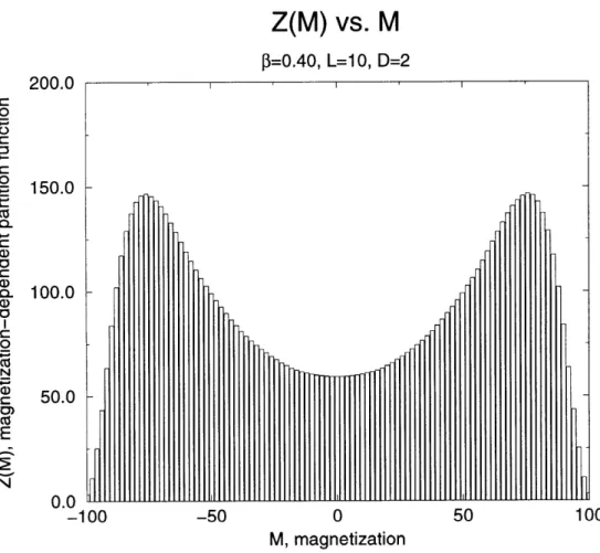
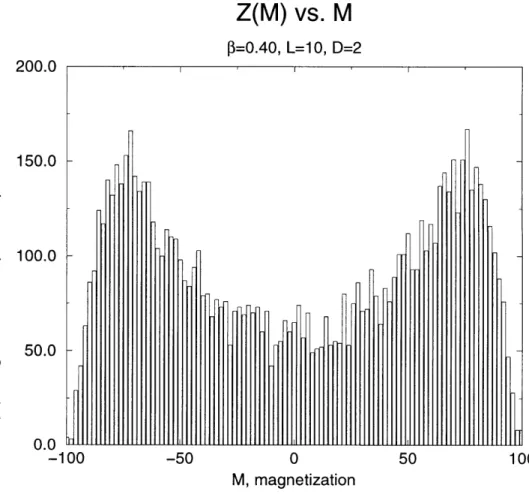
The two dimensional Ising Model was then investigated using a multi-cluster algo-rithm. Small lattice sizes (L < 10) were used at first to continue testing the accuracy of new implementations. The first implementation was the improved estimator for (M), mentioned in Section 3.3.1. Once this part was working correctly, then a routine was added to histogram the magnetization of the configurations. Then the second improved estimator for the partition function was included. Data was compared be-tween the two codes, the one with the improved estimator and the one without it. In Graphs A-8 and A-9, the effect of this improved estimator is to smooth the histogram out, giving a more accurate description of the partition function.

Now increasing the statistics of the two phase configurations was taken into ac-count. The trial distribution was implemented into the program, including the added Metropolis step mentioned in Section 3.4.1. By setting the trial distribution to a con-stant value of 1, the effect of the trial distribution would be negated and the results should be exactly the same if there was no trial distribution. This fact was checked and confirmed.

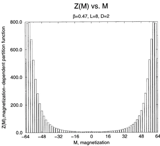
The best Ansatz for the trial distribution was figured to be the actual histogram of the magnetization itself. Thus a small Monte Carlo run was done and the histogram from that run was used to be the trial distribution of a larger Monte Carlo run. This worked very well for small lattice sizes, shown in Figures A-10 and A-11. Normal-ization was done so that the total number of counts in each histogram was equal to the number of Monte Carlo steps, although each histogram can be normalized to any value necessary.

However, in the runs of the larger lattice sizes (L > 14), it was found that a small Monte Carlo run would not generate a full histogram to use a trial distribution. The

histogram of the magnetization would have zero values because even with the tech-niques implemented, the program would not be able to generate some configurations due to their exponentially suppressed probabilities. To overcome this problem, an Ansatz of the trial distribution was used, generated from the proposed formula of the partition function from Professor Wiese's theory [3]. The accuracy of this Ansatz trial distribution had to be calculated carefully because a large error in the calculation was found to occur if the Ansatz distribution had the wrong magnitude in the region of magnetization of the two phase configuration. With this adjustment made, larger lattice sizes could be investigated.

Another step to improve accuracy was the use of the previous magnetization par-tition function for the trial distribution. Once the magnetization-dependent parpar-tition function was calculated, it became the trial distribution for the next run. This al-lowed the improved accuracy of previous runs to be carried along to improve the next run.

4.2

Results

Tables B.2, B.3, and B.4 contain data from various runs at different O's and L's and the observables calculated from each. In total, 17 different lattice sizes and 3 different values of 3 were run using this method. The lattice sizes ranged from 2 to 100 and the values of / used were Tc (the critical temperature, about 0.44), 0.47, and 0.50. Comparison to other research to measure the same observables showed good agreement [5].

One data file was used for data input and three files were used for output data.

The input data file contained the lattice size, L, the inverse temperature,

/,

and the

number of Monte Carlo steps to be used to generate the trial distribution and the magnetization-dependent partition function. One output file contained the values for the magnetization and susceptibility calculated for each run. From the magnetiza-tion histogram, the interface tension was extrapolated using Equamagnetiza-tion ( 2.10) and then written to another output data file. The last file held the histogram for the

magnetization-dependent partition function.

The surface tension from the data approached the analytical value in agreement with Onsager's calculation[l] in the runs with the large lattice size, as shown in Figures A-12, A-13, and A-14. With this information, the interface stiffness was extrapolated to the infinite volume limit by use of a fit to a form from a rearrangement of Equation (2.10) His theory predicts that a --+ o' + a/L, with a' being the ratio of values from the magnetization-dependent partition function.

4.2.1

Statistical Errors: Monte Carlo

The Monte Carlo method is an approximation of an infinite calculation. It calculates observables in a finite number of steps that are truly represented by average measure-ments on a system in equilibrium forever. These errors are statistical in nature.

The naive error of the magnetization is, from basic principles:

AM = '(M 2_{) - (M)} 2 _(4.1)

It assumes that the measurements taken are independent and have no correlation. For the multi-cluster algorithm, this level of error analysis is sufficient because of the lack of correlation between measurements.

The error in the susceptibility from Monte Carlo statistics is given by

Ax = (M 4) - M22 (4.2)

These equations are used to calculate the error in the magnetization and suscep-tibility from the Monte Carlo simulations.

4.2.2

Statistical Errors: General

These general statistical errors occur in the actual calculation of measured values. Using a process called "bining", the observables were calculated five to ten times for each f and lattice length L at a smaller number of Monte Carlo steps rather

than one large Monte Carlo run. This is to remove correlations that may be in the measurements. A statistical average is taken for the multiple values taken from each particular pair of parameters and this value is used.

4.2.3

Systematic Errors

The general reasoning of this method of calculation is based on an expansion of a mathematical description of the actual possible configurations. The method pre-sumes that beyond the critical temperature to the lowest order, the configuration either forms one large domain or creates two separate phase domains. This gives three basic areas of contribution to the magnetization-dependent partition function:

two around the plus and minus values of the average magnetization (M = ±(Mavg))

and one around zero (m = 0). The expansion is for large volumes and

configura-tions of magnetization near zero. This is why an extrapolation from small to large volumes is necessary. To higher orders, however, combinations of these two types of configurations are possible. There could be a large domain of one phase inside the opposite phase and an interface. There could be multiple interfaces or domains. These configurations are not accounted for at this level of the expansion and could have contributions to the regions not covered by the expansion.

Chapter 5

Conclusion

The goal of this thesis was the development of a method of calculation for certain observables of the Ising Model in any dimension through the use of a two dimen-sional test case. Many methods were used to do this. A combination multi-cluster and Metropolis algorithm using a trial distribution to increase the statistics of cer-tain states was developed. Two improved estimators were implemented: one to help measure the susceptibility which relies on (M) and one to build a histogram of con-figurations separated by magnetization. A theory by Professor Wiese [3] was used to build an Ansatz and calculate the results to compare with previous work. The results for this test case have shown that the method does work and agrees with previous calculations by Onsager [1].

What makes this work unique is not the use of improved estimators or a trial distribution but the use of the combination of both. As of this time, this is the first attempt at such an approach and the improvement of data that it allows. One of the main concerns about using the Monte Carlo method to accumulate data is how long to run, that is, how many Monte Carlo steps are necessary until accurate data can be taken. This method allowed for a reduction of Monte Carlo steps, or equivalently an increase in the accuracy of the Monte Carlo calculation. The rough estimate of efficiency is about a order of magnitude of the number of Monte Carlo steps when compared to the work of others who did not use cluster algorithms to

Now, our method can be used to calculate properties of the Ising Model in higher dimensions. The Monte Carlo methods used can be extended to higher dimensions with little work. However, deeper analysis of the Ising model in higher dimensions is necessary to understand how the characteristics of interface tension and stiffness can be calculated from magnetization-dependent partition functions.

I would like to thank my Advisor, Professor Uwe-Jens Wiese, for his constant support and guidance throughout this thesis.

Appendix A

Figures

interfaces

OLI

"up" spin

M

"down" spin

Figure A-i: Two regions of different spins separated by two interfaces

4/

4/

S1 S2 S3 S S n+ S1

I

I

I I

I

I

I I I

I

ID Ising model

SS2 Si3 Sin n+1 = Sil

)2

n

)n+l

Ss1

2D Ising model

Figure A-4: Two phase configuration

I I

N

ON

I

I I

U

ON

Z(M) vs. M

without trial distribution

M, magnetization

Figure A-6: Original magnetization-dependent partition function, Z(M) 0.80 0.60 0.40 0.20 0.00 U -1 III 00 -50 100 I I I '''''''''"'''''''''''''"''' milli I 111111111,111111111111111 lint,'''''''

Zeff(M)

vs.

M

with trial distribution 0.0200 S0.0150 0 t " 0.0100 0.0050 0.0000 -100 -50 0 50 100 M, magnetization

Z(M) vs.

M

P=0.40, L=10, D=2

-50 0 50 100

M, magnetization

Figure A-8: Effect of the improved estimator: with improved estimator 200.0 150.0 100.0 50.0 0.0 LU -100

Z(M) vs. M

3=0.40, L=10, D=2

-50 0 50 100

M, magnetization

Figure A-9: Effect of the improved estimator: without improved estimator 200.0 150.0 100.0 50.0 0.0 [dl -100

Z(M) vs. M

3=0.47, L=8, D=2

-48 -32 -16 0 16 32 48 64

M, magnetization

Figure A-10: magnetization-dependent partition function for 3 = 0.47, L = 8 800.0 600.0 400.0 200.0 0.0 ELL -64

Z(M) vs. M

3=0.47, L=12, D=2 500.0 400.0 300.0 200.0 100.0 0 .0 11111 "1 1111 'l"1111,1111111... -144 -108 -72 -36 0 36 72 108 144

(;vs.

L

J3Tc(0.44086), D=2 0.60 [---F measured values W - analytical value 0.40 -C ® 0.20 0.00 -0.20 I 0 20 40 60 80 100 L, lattice length

( vs.

L

f=0.47, D=2

Figure A-13: The 0.80 0.70 0.60 0.50 0.40 0.30 0.20 0.10 0.00 0.0 40.0 60.0 80.0 L, lattice length

surface tension for 3 = 0.47

( vs.

L

3=0.50, D=2

i-A measured values analytical value 'N U I I I I 8 0 I 0.80 0.70 0.60 0.50 0.40 0.30 0.20 0.10 0.00 20 40 60 80 L, lattice length

Figure A-14: The surface tension for / = 0.50

100

Appendix B

Tables

Table B.1: Magnetization (M) and susceptibility X data from D = 1, L = 4 Cluster algorithm No. of steps 1x106 1x106 1x106 1x106 1x106 1x106 1x106 1 x 106 1x106 1x106 1x106 Ix106

(M)

-0.1225(5) 0.8745(6) 0.0165(6) -0.3005(6) -0.0215(7) 0.1390(8) 0.3395(8) -0.2385(9) -1.8300(9) 1.1000(9) -0.2520(10) X 0.2500(3) 0.3055(3) 0.3713(4) 0.4488(4) 0.5333(4) 0.6202(4) 0.7028(4) 0.7756(4) 0.8350(3) 0.8821(3) 0.9174(3) X, Analytical 0.2500 0.3052 0.3718 0.4490 0.5337 0.6203 0.7025 0.7751 0.8351 0.8821 0.9172 0.000 0.000 0.100 0.200 0.300 0.400 0.500 0.600 0.700 0.800 0.900 1.000

Table B.2: Surface tension o, magnetization (M), and susceptibility X for D=2, f3TC L No. of steps a (M) x 2 100000 0.5201 0.0019(83) 0.6816(8) 4 100000 0.4171 -0.0027(73) 0.5323(15) 6 100000 0.2697 -0.0020(69) 0.4766(17) 8 100000 0.2010 0.0030(67) 0.4515(18) 10 100000 0.1576 -0.0034(66) 0.4318(19) 12 100000 0.1305 0.0030(65) 0.4185(19) 14 100000 0.1134 0.0001(64) 0.4112(20) 16 100000 0.0976 -0.0035(63) 0.4033(20) 18 100000 0.0877 -0.0025(63) 0.4005(21) 20 100000 0.0781 -0.0046(63) 0.3965(21) 30 100000 0.0533 -0.0473(63) 0.4147(22) 40 100000 0.0195 0.0997(50) 0.6530(8) 50 100000 0.0157 0.0981(49) 0.6438(7) 60 100000 0.0130 -0.2984(48) 0.6356(7) 74 100000 0.0103 0.1009(48) 0.6239(7) 80 100000 0.0096 -0.3027(48) 0.6203(6) 100 100000 0.0029 0.0002(53) 0.4407(9) exact 0. 0.

Table B.3: Surface tension a, magnetization (M), and susceptibility X for D=2, 0 = 0.47 No. of steps 100000 100000 100000 100000 100000 100000 100000 100000 100000 100000 50000 50000 50000 50000 50000 50000 50000 a0 0.5858 0.4937 0.3697 0.2986 0.2592 0.2309 0.2120 0.1968 0.1876 0.1787 0.1416 0.1289 0.1402 0.1259 0.1342 0.1262 0.1149 0.11491859

(M)

0.0003(83) 0.0029(74) -0.0063(71) 0.0040(70) -0.0017(69) 0.0000(69) 0.0035(69) 0.0046(69) -0.0066(69) 0.0057(69) 0.0879(61) 0.1925(63) 0.1598(70) -0.1202(64) -0.1638(54) 0.1631(59) 0.3097(62) 0. L 2 4 6 8 10 12 14 16 18 20 30 40 50 60 74 80 100 exact x 0.6910(8) 0.5528(14) 0.5099(15) 0.4914(16) 0.4823(17) 0.4743(17) 0.4707(17) 0.4705(17) 0.4710(17) 0.4709(16) 0.6313(8)3 0.6043(12) 0.5925(13) 0.6507(10) 0.7100(11) 0.6594(12) 0.6208(8)

Table B.4: Surface tension a, magnetization (M), and susceptibility X for D=2, S= 0.50 No. of steps 100000 100000 100000 100000 100000 100000 100000 100000 100000 100000 50000 50000 50000 50000 50000 50000 50000 a 0.6495 0.5787 0.4772 0.4008 0.3624 0.3363 0.3152 0.3040 0.2982 0.2910 0.2759 0.2525 0.2281 0.2281 0.2281 0.2281 0.2281

(M)

-0.0009(84) -0.0045(76) 0.0032(73) -0.0028(73) -0.0110(72) -0.0028(72) 0.0085(72) -0.0006(72) 0.0100(73) 0.0053(73) -0.0037(73) 0.1535(72) 0.4431(56) -0.0391(56) -0.0598(52) -0.0767(47) 0.1272(44) exact 0.228063166 0. L 2 4 6 8 10 12 14 16 18 20 30 40 50 60 74 80 100 X 0.7001(6) 0.5743(12) 0.5395(13) 0.5275(14) 0.5194(13) 0.5224(13) 0.5203(12) 0.5190(10) 0.5391(11) 0.5401(9) 0.5441(10) 0.6318(14) 0.6842(9) 0.7084(8) 0.6834(10) 0.5983(16) 0.5997(14) exact 0.228063166 0.

Bibliography

[1] L. Onsager. Two dimensional ising model. Phys.Rev., 1944.

[2] R. H. Swendsen and J.-S. Wang. Nonuniversal critical dynamics in monte carlo simulations. Phys.Rev.Lett., 1987.

[3] U.-J. Wiese. Capillary waves in binder's approach to the interface tension. hep-lat/9209006.

[4] J. M. Hammersley and D. C. Handscomb. Monte Carlo Methods. Chapman & Hall, 1983.

[5] B. A. Berg, U. Hansmann, and T. Neuhaus. Properties of interfaces in the two and three dimensional ising model. Z.Phys.B, 1993.