Canonical correlation of shipping forward curves

(1)

CANONICAL CORRELATION OF SHIPPING FORWARD CURVES

By

Nicholas A. Hadjiyiannis

MEng., Mechanical Engineering with Transport Engineering, Imperial College London (2006) S.M., Transportation, Massachusetts Institute of Technology (2007)

S.M., Naval Architecture and Marine Engineering, Massachusetts Institute of Technology (2009) MBA, Business Administration, Harvard Business School (2010)

PhD, Mechanical Engineering, Massachusetts Institute of Technology (2010)

Submitted to the Department of Mechanical Engineering In Partial Fulfillment of the Requirements for the Degree of

Master of Science in Ocean Engineering MASSA( At the

Massachusetts Institute of Technology

N

September 2010

LI

The author hereby grants to MIT permission to reproduce and to distribute publicly paper and electronic copies of this thesis document in whole or in part

in any medium now known or hereafter created.

ARCHNES

CHUSETTS INSTITUTE F TECH'LO-Y

3V

0 4 2910

PRR ES Signature of A uthor... ... ... Department of Mechanical Engineering

July 29, 2010

Certified by... ...

Paul D. Sclavounos Professor, Department of Mechanical Engineering Thesis Supervisor Accepted by

David Hardt Professor of Mechanical Engineering Chairman, Department Committee for Graduate Students

(2)

CANONICAL CORRELATION OF SHIPPING FORWARD CURVES

By

NICHOLAS A. HADJIYIANNIS

Submitted to the Department of Mechanical Engineering

on 2 9th July 2010 in partial fulfillment of the requirements for the Degree of

Master of Science in Ocean Engineering ABSTRACT

The behavior and interrelations between the main shipping forward curves are analyzed using multivariate statistics after removing the volatility distortions dictated by the Samuelson hypothesis. Principal Components Analysis and Canonical Correlation analysis were used to demonstrate how the task of explaining the various shipping forward curves can be simplified substantially and how very high correlations can be achieved between shipping forward curves. The conditions under which correlations are higher are discussed as well as the various applications of these results using case studies. Applications include trading from a hedge fund perspective, cross hedging any physical exposure in illiquid markets and portfolio optimization. Conditioning as a tool is also examined to demonstrate how more reliable correlation results can be obtained for cross-hedging or other purposes, and how the best trading opportunities can be unveiled conditional on recently observed data. Tanker valuations are carried out using the adjusted forward curves with the RAFL ship valuation model. The results are very close to transaction prices for relatively modem vessels while deviations in older ships are explained with regards to phase out regulations and other factors. The ship value volatility and consequently the valuations of typical options are substantial and increase as a percentage of the ship value with age. These results have to be considered seriously in shipping transactions that include optionalities which are very common.

Thesis Supervisor: Paul D. Sclavounos

(3)

Acknowledgments

First and foremost I would like to thank my supervisor Professor Paul D. Sclavounos for his valuable guidance in my research. I would also like to thank Vassilis Karakoulakis of Clarksons and Per Einar Ellefsen of Arrowhawk Capital Partners for the data that was used in the preparation of this thesis.

(4)

Abbreviations

BCI: Baltic Capesize Index BOD: Board of Directors BPI: Baltic Panamax Index

CAPE: Capesize Bulk Carrier (~175,000dwt) CCA: Canonical Correlation Analysis FFA: Forward Freight Agreements MR: Medium Range Tanker

PCA: Principal Components Analysis PMX: Panamax Bulk Carrier (-75,000dwt)

RAFL: Risk Adjusted Forward Looking Ship Valuation Model S&P: Sale and Purchase

SVD: Singular Value Decomposition

TC: Tanker - Clean (Products) 4TCA: 4-Route Time Charter Average TCE: Time Charter Equivalent TD: Tanker - Dirty (Crude Oil)

VLCC:Very Large Crude Oil Carrier (~200,000dwt -300,000dwt) WS: Worldscale

(7)

1. Introduction

The purpose of this thesis is to analyze the behavior and interrelations between the main shipping forward curves and then use them for tanker valuations. Five high liquidity dry bulk and tanker routes were chosen as summarized in Table 1.1.

ROUTE DESCRIPTION

BCI TCA: Average time charter earnings on the four main Cape routes BPI TCA: Average time charter earnings on the four main Panamax routes TD5: Suezmax -Crude Oil from West Africa to East US Coast TD3: VLCC -Crude Oil from Saudi Arabia to Japan

TC2: MR Product Carrier -Clean Product from Rotterdam to New York

Table 1.1: Chosen Shipping Forward Curve Routes

The Baltic publishes indices for these routes on a daily basis and futures are traded on these indices either over the counter or through clearing houses. Contracts of various tenors are traded daily that span out to 2 - 5 years. Note that these are Asian

futures that settle over a period as opposed to a particular date. Data was collected on contracts of the various tenors on the above routes. This data is in the form of time series of daily futures prices from February 1 0th 2005 to July 2 9th 2010.

The traded futures have fixed maturity dates, so the time to maturity decreases with time. It is well known that the volatility of futures prices increases as we approach maturity by virtue of the Samuelson hypothesis i.e. due to reasons including the increased information for the immediate future [Samuelson 1965]. We want to exclude this effect so we can analyze the data and its volatility more effectively. The first step of the analysis, therefore, is to create new time series of prices for contracts with a continuously rolling tenor, meaning that the time to maturity is kept constant.

Using the continuously rolling contracts, Principal Components Analysis (PCA) will be carried out to identify the number of factors required to explain an adequate amount of the variance of these forward curves. Canonical Correlation Analysis (CCA)

(8)

will then be applied to determine the maximum possible correlation between those forward curves and how that can be achieved. Finally, tanker valuations will be carried out using the rolling contracts with the Risk Adjusted Forward Looking (RAFL) ship valuation model which was originally developed by [Hadjiyiannis 2010] for the valuation

(9)

2. Canonical Correlation Analysis (CCA)

Using CCA, we can determine the maximum possible correlation between two sets of variables and the way that can be achieved. In our case, we will be maximizing the possible correlation between various shipping forward curves. The two sets of variables in this case are two portfolios of futures contracts with various tenors. The applications of this analysis are discussed in Section 6. They include cross hedging in markets where a illiquidity prevents a "perfect" hedge, trading from a hedge fund perspective etc. What follows is a brief mathematical explanation of canonical correlation analysis and the way it can be applied to our particular problem.

Consider 2 sets of variables e.g. one set of futures for Capesize bulk carriers,

(C,, C2 ,---- C,) and one set of futures for Suezmax Tankers (S,, S2 ,--- S,). Denote the

number of variables in the two datasets as p, and p2 respectively, where p, p2 and

assume these variables are measured about their means. The data for each variable is recorded as a time series over a period of "n" days. The data matrix can be written in a vertically partitioned form where [C] is (n x p,) and [S] is (n x P2)

[X]

C

(2.1)

I[S])

The Covariance matrix is also partitioned as follows:

[

E]l=

1

(2.2)

[Y-1] [Y-22]1

We want to find the maximum possible correlation between a portfolio of Cape futures ii with weights d and a portfolio of Suezmax futures i with weights

pi.

i = a1C, + a2C2 +...+ aC, = da [C] (2.3)

(10)

For simplicity, we standardize both linear combinations to unit variance:

var(i)=E(i2) =E(dT [C][C]T d) =i T [y]=1 var()= E

(i;2)

=

E

(T

[S][S]T

)

[1

₂

]

1 Since the variables are zero centered, we have: E

(

Therefore, the Correlation between u and v is given by:

E({ii)

= E(dT

[C][S]

T

i)

=

T

(2.5)

(2.6)

(2.7)

(2.8)

Equation 2.8 is to be maximized subject to the constraint that ii and j are unit vectors (Equations 2.5 and 2.6). We use the Lagrangian expression,

T

_[E

_] _-1)-_{_)} _p(4 _[X-1 _- _(2.9)

where A and p are Lagrangian multipliers. Note that subject to constraints (2.5) and (2.6), yV is equal to the correlation (Equation 2.8). We maximize yf by differentiating with respect to vectors d and

p

, and setting the derivatives simultaneously equal to zero:

a _a =[ Z1 2] -2[Z]dT =0 (2.10)

=[E12]T d- p[E22j 0

ap

Combining with constraints 2.5 and 2.6 (unit variance), we get:

(2.11)

(11)

TCV =d[Z]J-2(1)=0 (2.12)

ad

T O/= j [E-1 ]Td S-p(1) = 0 (2.13)

a~d

Combining (2.12) and (2.13) yields:

A = p = iiT [YE-1|2j(2.14)

From equation (2.8) and (2.14), we see that the Lagrangian multiplier k is equal to the correlation between the two data sets. Since[ 12]T =[21], we can rewrite (2.10) and

(2.11) directly in matrix form as follows:

A[Y2[11] [2]fa ₀

(2.16)

[Yx2 1]1 A[ 22Jkj3J =

The combined vector in Equation 2.16 contains the portfolio weights of the two data sets (e.g. Capes and Suezmax Tankers) and is of length p + P2 . Denote this as vector

- and the partitioned matrix preceding it, matrix[A]. Rewriting Equation 2.16, we have:

[A] = 0 (2.17)

Note that this is not a classical Eigenvalue problem because [A] is a block matrix in which the X values also lie off the diagonal. Equation 2.17 has to be solved for the p,+ P2possible non-trivial pairs of ) and i . The largest real value of X is the maximum attainable correlation between the two data sets and the corresponding portfolio weights are defined by Equation 2.17 for a given X. There are two ways to proceed from this point to solve Equation 2.17.

(12)

Method 1.

By further manipulation, we can reduce Equation 2.16 into a classical Eigenvalue problem and then solve for the Eigenvalues and Eigenvectors. We start by breaking

Equation 2.16 back into equation form:

-A [El 1"+ [E2 = 0

z

21 ~ A-

22] =

0

(2.18) (2.19)

We then Multiply Equation 2.18 by the inverse of matrix [E,] and Equation 2.19

by the inverse of matrix

[YE1]

to get:

-A [ I] 5+( E-:|1 E1 =0

(E 21 -A[7]f= 0

(2.20) (2.21)

Equations 2.20 and 2.21 can now again be written in partitioned block matrix form as follows:

LI[12]

0

_. )-A . =0 (2.22)

0

EzNIz2 2

Note that the block matrix multiplied by k is simply the identity matrix, while the joint vector following it is vector fv. Naming the new block matrix on the left

[B],

we are left with:

-> [B - AI] 0 (= (2.23)

(13)

This is a simple Eigenvalue problem with the Eigenvalues lying only on the diagonal. Therefore, it can simply be solved on MATLAB for the Eigenvalue / Eigenvector pairs. We are interested in maximizing the correlation between the two data sets so we chose the pair involving the highest real Eigenvalue.

Note that[E21

]

= [ _{1 2}] T, but

[EI]

is unrelated to[E2 2

],

since the two matrices are

each wholly derived from two separate sets of variables. That means that matrix [B] is not symmetric, even though its Eigenvalues are real.

Method 2.

For non-trivial solutions of Equation 2.17, we set the determinant of matrix [A] equal to zero to get a polynomial of order p, + P2 which is then solved for p, + P2 values

of k. We select the highest value of k which is the maximum correlation. Call this A* and the corresponding vector of portfolio weights i*. In equation terms:

Solve directly for k:

Maximum correlation:

Substitute A* into (Eq. 2.17):

-A [Y-1 ] [Y-12]

*

12

1 X

-

-[-22]

-o

A*

=

MAX(-2 I 21.. 'An)

2A*[Eij]

[Y-12]

This is simply Equation 2.16, but now with a known value of k. In other words, all the elements of matrix [C] are known. The only unknown in Equation 2.26 is the vector _*. This cannot simply be solved as a system of simultaneous equations using singular value decomposition (SVD) because by definition, two of the equations are

(2.24)

(2.25)

(2.26) , Y-12 " * = [C ] *0

(14)

interdependent (we don't know which). There are infinite solutions since vector w* can take any magnitude. However, also by definition, matrix [C] will have an Eigenvalue which is equal to zero and we can use that as follows:

Solve the Eigenvalue Problem for matrix[C], to get Eigenvalues "k" and Eigenvectors e: Eigenvalues (k) from: Eigenvectors ( ) from: [C] -k[J]I -2* [F ] -k [ 12 ] [Y-] - *[=0-([C] -k [I]) = [11 (2.27) , 2 j

= 0

(2.28) -A* [22|-k,

By definition, the eigenvector corresponding to k=0 satisfies the equation:

[C]2

=

2 = 0

(2.29)

Note that Equation 2.29 is the same as Equation 2.26. In other words:

w* =e2 (2.25)

So, all we have to do to find the vector of portfolio weights v* after finding *, is solve the Eigenvalue problem for matrix [C] and select the Eigenvector that corresponds to the zero Eigenvalue.

(15)

3. Principal Components Analysis (PCA)

PCA will be carried out in order to identify the number of principal components necessary to explain an adequate portion of the variance of the main shipping forward curves. PCA is analogous to a canonical correlation of the data set with itself. In simple terms, PCA maximizes the variance of the data set. The Eigenvalues of the covariance matrix correspond to the maximum variance while the eigenvectors correspond to the portfolio of variables that achieves that variance.

A brief mathematical explanation along the lines of the canonical correlation analysis goes as follows. We start with a set of p zero-centered variables e.g. a set of futures series for Capesize bulk carriers, (C,,C 2 ,----, C,). Now [X] has p components

and the covariance matrix

[Z].

We want to find a weight vector d which maximizes the variance of the portfolio, subject to the constraint:

dra =1 (3.1)

The variance of the portfolio is given by:

E

(iT

[X])

2 = E(diT [X] [X]T

i) = i& (3.2)

Again, we introduce a Lagrangian multiplier A:

iT

= y']S -i A(ii'5 - 1) (3.3)

Note that the Lagrangian expression reduces to Equation 3.2, subject to constraint 3.1. Next, we maximize the variance by differentiating the Lagrangian expression with respect to vector

a

and setting the derivative equal to zero:

(16)

/ = 2

[ZL ]

d - 2 Ad = 0 (3.4)

a

Multiplying Equation 3.4 by

a",

and combining with Equation (3.1) we get:

a

T [E ] d

= Aa

i = A (3.5)

From 3.2 and 3.5, we see that the Lagrangian multiplier A is equal to the variance of the portfolio, in much the same way as it was equal to the correlation between the datasets in the CCA. This time, however, the analysis is much simpler as Equation 3.4, directly reduces into an Eigenvalue problem described by Equation 3.6.

(z

- AI) = 0 (3.6)

More can be read about PCA and Canonical Correlations in [Basilevsky 1994] and [Anderson 2003]. The Singular Value Decomposition (SVD) of the covariance

matrix

[E]

takes the form:

[y]

= [U]T [A][U] = [V][V]T, where [V] = [U][A]112 (3.7)

[U] is the matrix containing the Eigenvectors of

[Z]

and [A] is the diagonal matrix containing its Eigenvalues. Equation 3.7 tells us that the volatility of an independent statistical factor, as it affects the ith price series is equal to the square root of the Eigenvalue corresponding to that factor, multiplied by the ith element of the corresponding Eigenvector.

Since the factors are independent Gaussian random variables, we know that that the total variance is equal to the sum of the variance by each factor. So the variance

explained by each factor is simply the Eigenvalue corresponding to that factor, divided by the sum of the Eigenvalues. The shape of the corresponding Eigenvector then tells us how that factor affects the contracts of various tenors.

(17)

4. Data Analysis and Procedure

4.1 Procedure Overview

The first big part of the analysis is the calculation of the covariance matrices that will be used in both the canonical correlation and principal components analysis. This can be broken down into five steps.

The raw data is in the form of time series of futures prices with various tenors. The expiration period of these futures is defined by the trading date and a set of rules that vary between trading houses and over time. The first step of the analysis is to determine the precise expiration dates of all the fixed futures contracts for each day throughout the time series. The expiration periods are months, quarters or years, but they are always fixed meaning that they always start on the first trading day of the first month of the expiration period.

The next step is to create a new set of futures price series for fictitious contracts that have a continuously rolling tenor i.e. a constant time to maturity. This will remove the effect of volatility increasing as maturity is approached (Samuelson hypothesis).

For the dry bulk routes, futures prices are quoted $/day whereas for tanker routes, they are quoted in worldscale. Worldscale is a percentage of a flat rate which is quoted in $/ton and is updated every year for each route. In order to carry out the canonical correlation analysis between bulk carrier and tanker routes, we have to convert the tankers time series from worldscale to time charter equivalent (TCE). We do that using the specifics of each route (miles, port fees etc) and time varying quantities including

each year's flat rate and bunker prices.

The next step is to zero-center the original data for the "trended" volatility, and to zero-center the log differences of the data for the "de-trended" volatility.

Finally, we combine the series to produce covariance matrices for each individual dataset and for each dataset pair. These will then be used directly in the PCA, or combined with others to form the block matrices that are used in the CCA.

(18)

4.2 Creation of Continuously Rolling Contracts

The objective of this section is to use the prices of fixed maturity contracts in order to determine the prices of contracts with continuously rolling maturity dates (rolling contracts). This has to be carried out for each day in the time series. Taking the CAPE 4TCA for example, on a given business day there are futures prices quoted for the next month (M+1), the month after that, the next quarter (Q+1) and the next 5 quarters after that (Q+2 to Q+5), the next year (Y+I1) and the 4 years after that (Y+2 to Y+5). We want to use those prices to determine the prices for the first quarter starting today (RI), the quarter beginning exactly one quarter from today (R2) etc. Note that on any given day, the maturity periods of the rolling quarters will overlap with those of fixed periods. In

other words, the rolling contracts are combinations of fixed contracts.

There are various methods that can be used to solve this. One of the most intuitive is to assign a price to each future day based on the fixed contracts and then take the average across the days that lie in the rolling quarter in order to get the price of the rolling quarter. That is essentially taking a weighted average. A more robust and efficient method involves linear interpolation between fixed contracts. This is summarized in the

following three steps:

Step 1:

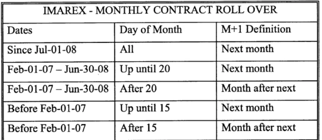
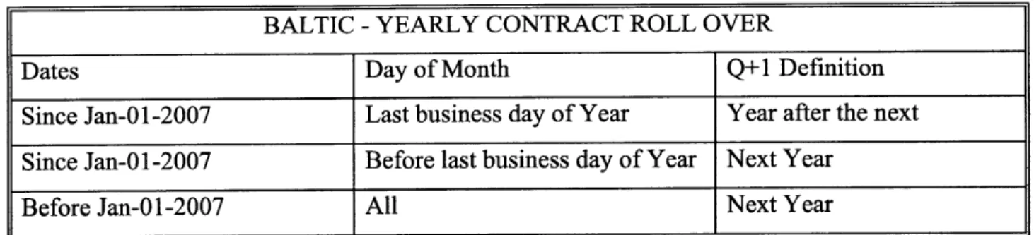
First we determine the precise maturity dates of the fixed contracts. The days on which the roll-over occurs (definition of M+1, Q+1, Y+1 etc. on any given date) differs between clearing houses and has also changed on several occasions in the past. The data on tanker futures is from IMAREX and the data on dry bulk futures is from the Baltic Exchange. Tables 4.1 to 4.5 summarize the roll over rules for both throughout the period over which the data was collected.

Note that fixed contracts always start on the 1st day of the month. M+2 is always

the whole month after M+1, Q+2 is the whole quarter after Q+1, Y+2 is the whole year after Y+1, M+3 is the whole month after M+2 etc. This means that the roll over rules for all the contracts can be defined by those for M+1, Q+1 and Y+1.

(19)

IMAREX -MONTHLY CONTRACT ROLL OVER

Dates Day of Month M+1 Definition

Since Jul-01-08 All Next month

Feb-01-07 - Jun-30-08 Up until 20 Next month Feb-01-07 - Jun-30-08 After 20 Month after next Before Feb-01-07 Up until 15 Next month Before Feb-01-07 After 15 Month after next

Table 4.1: Roll Over Rules for Monthly Contracts of IMAREX

IMAREX - QUARTERLY AND YEARLY CONTRACT ROLL OVER

Dates Month Q+1 Definition Y+1 Definition

All 1, 4, 7, 10 Next Quarter Next Year

All 2,3,5,6,8,9,11,12 Quarter after next Next Year

Table 4.2: Roll Over Rules for Quarterly and Yearly Contracts of IMAREX

BALTIC -MONTHLY CONTRACT ROLL OVER

Dates Day of Month M+1 Definition

Since Jan-01-2007 Last business day of month Month after the next Since Jan-01-2007 Before last business day of month Next month

Before Jan-01-2007 All Next Month

Table 4.3: Roll Over Rules for Monthly Contracts of the Baltic Exchange

BALTIC - QUARTERLY CONTRACT ROLL OVER

Dates Day of Month Q+1 Definition

Since Jan-01-2007 Last business day of Quarter Quarter after the next Since Jan-01-2007 Before last business day of Quarter Next Quarter

Before Jan-01-2007 All Next Quarter

(20)

BALTIC - YEARLY CONTRACT ROLL OVER

Dates Day of Month Q+1 Definition

Since Jan-01-2007 Last business day of Year Year after the next Since Jan-01-2007 Before last business day of Year Next Year

Before Jan-01-2007 All Next Year

Table 4.5: Roll Over Rules for Yearly Contracts of the Baltic Exchange

Step 2:

In Step 1 we defined the precise expiration period for each futures contract on every day of the time series. Next, we define the mid-point of expiration for each contract on each day of the time series. That is simply taking the date that lies in the middle between the starting and ending dates of the expiration period. We assign the prices of the futures contracts to their mid-point of expiration date. On each given day we will have values for various future dates. These points will be from monthly, quarterly and yearly contracts. Then we join these points to create a futures curve using linear interpolation. Other functions could be used here but linear interpolation is simple and robust.

Step 3:

The next step is to determine the mid-point of expiration date for the rolling contracts that we want to price. For example, the mid-point of expiration date for the first rolling quarter (R1) will be exactly half a quarter from today. Then the mid-point of expiration for R2 will be one quarter after that and so on. Having defined the mid-point of expiration dates for the rolling quarters in each day of the time series, we go back to

Step 2, and interpolate for the corresponding futures prices.

Note that it is important to only interpolate - not extrapolate, particularly when using linear interpolation, because the gradient of the forward curve can be quite steep at some points leading to extreme results by extrapolation. Following this procedure, we create time series for the rolling contract futures prices spanning over the same time frame as the initial data. That is from Feb-10-2005 to July 29 2010 for 10 rolling quarters in all datasets, and from March-10-2008 to July-29-2010 for 22 rolling quarters for the dry bulk futures.

(21)

4.3 From Worldscale to Time Charter Equivalent

As explained earlier, tanker futures are quoted in worldscale, which is a percentage of a flat rate. The flat rate is a nominal value of $/ton, updated every year to reflect changes in bunker costs and other expenses. The annual updating of the flat rate is not reflected in our time series of futures that are quoted in worldscale. Therefore, it would make no sense to carry out a CCA between tanker futures quoted in worldscale and dry bulk carrier futures which are quoted in $/day. We must first convert everything to time charter equivalent ($/day) for the comparison to make sense. To convert from worldscale (WS) to time charter equivalent (TCE) we use Equation 4.1.

TCE =- FWT (l-C)-Bb--P-0 4.1

d 100

TCE: Time Charter Equivalent ($/day) d: Total Return Voyage Days F: Flat Rate ($/ton)

W: World Scale

T: Cargo Transported (tons) C: Commissions (%)

B: Total Bunker Consumption (tons) b: Bunker Price ($/ton)

P: Port Costs in Load and Discharge Ports

($)

0: Other Costs ($)

All the parameters are defined for the return voyage. In other words, when calculating duration, consumption and other parameters for each route, we assume that the ship will load at the origin, sail to the destination, discharge, and then return in ballast to where it started.

(22)

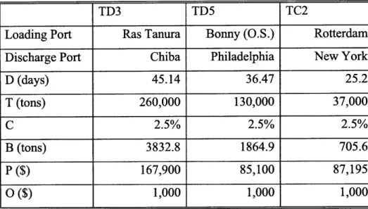
The parameters in Equation 4.1 are different for each route and also vary over time. For each route, the prevailing worldscale rate (W) changes daily, the bunker price (b) and the flat rate (F) change annually, and the remaining parameters remain constant. Table 4.6 provides a summary of the constant parameters for the selected tanker routes.

TD3 TD5 TC2

Loading Port Ras Tanura Bonny (O.S.) Rotterdam

Discharge Port Chiba Philadelphia New York

D (days) 45.14 36.47 25.2 T (tons) 260,000 130,000 37,000 C 2.5% 2.5% 2.5% B (tons) 3832.8 1864.9 705.6 P ($) 167,900 85,100 87,195 O

($)

1,000 1,000 1,000

Table 4.6 Constant Parameters for Worldscale to Time Charter Equivalent Conversions [Data from Clarksons 20101

Table 4.7 shows the bunker prices (b) at the assumed bunkering ports various routes every year. Note that bunker prices for future years are based on prices for bunkers at the relevant ports.

for the futures

Table 4.7 Bunker Costs for the Selected Tanker Routes Since 2005 [Data from Clarksons 20101

TD3 TD5 TC2

Bunker Port Fujairah Rotterdam Rotterdam

2005 256,590 233,979 233,979 2006 310,881 293,040 293,040 2007 373,746 345,065 345,065 2008 509,354 471,909 471,909 2009 372,777 353,810 353,810 2010 467,354 447,450 447,450 2011 452,340 432,310 432,310

(23)

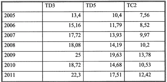
The flat rate of each year is based on the relevant costs for that route during the previous year until October. For example, the flat rate for the year 2011 will be based on bunker prices and other costs until October 2010. Therefore, as we approach October, our prediction of the next year's flat rate becomes more accurate. The flat rate is predominantly determined by bunker prices while other factors have a much smaller impact. Bunker futures are therefore also used to aid the predictions carried out before October. Table 4.8 shows the flat rates (F) each year for the selected trade routes.

TD3 TD5 TC2 2005 13,4 10,4 7,56 2006 15,16 11,79 8,52 2007 17,72 13,93 9,97 2008 18,08 14,19 10,2 2009 25 19,63 13,78 2010 18,72 14,68 10,53 2011 22,3 17,51 12,42

Table 4.8 Flat Rates for the Selected Tanker Routes Since 2005 [Data from Clarksons 20101

The major uncertainty in WS-TCE conversions of futures prices stems from the fact that the applied flat rate is the one prevalent upon expiration, which is often unknown at the time of contract. Therefore, an assumption is required to carry out the conversion. One could use the prevailing flat rate at the time of contract but that essentially assumes a constant flat rate until expiration. That is very crude since, as shown in Table 4.8, the flat rate has varied since 2005 by almost a factor of 2.

A more relevant assumption is that the actual flat rate was known in advance at the time of the contract. That means we convert futures contract prices to TCE in retrospect with the flat rates prevalent upon expiration. For contracts that are yet to expire, we can use current flat rate forecasts. This assumption is based on the fact that brokers provide a good estimate of the flat rate when closing a futures contract. These estimates are based on bunker prices and bunker futures prices, and have historically been very accurate.

(24)

4.4 The Covariance Matrix

Using the analysis described thus far, futures price series were created for 10 rolling quarters from Feb-10-2005 to July 29 2010 (1,383 trading days) in $/day for all 5 routes and in world scale for the 3 tanker routes. Futures price series were also created for 22 rolling quarters from March-10-2008 to July-29-2010 (605 trading days) for Capes and Panamaxes (distinguished by "22R") in $/day. That is a total of 10 datasets, 8 of which are (10x1383), and two of which are (22x605).

Next, we have to determine the covariance matrix for each individual dataset, and also between dataset pairs in order to create the block matrices required for the CCA. Note that each block matrix is composed of four covariance matrices. These are the two covariance matrices of the two individual datasets, a covariance matrix between the two datasets, and its transpose.

The analysis will be carried out using two different measures of volatility, so we will start by creating two sets of covariance matrices. The first set of covariance matrices derives from the de-trended daily log-differences of the futures price series. We call this the "de-trended volatility". The second set of covariance matrices is based on the measure of volatility by the standard deviation which, for lack of a better name, we call the "trended volatility".

One analogy that can be used to visualize the difference of the two volatility measures is that of short waves riding a long wave. The trended volatility is related to the departures of the free surface from the mean value of the long wave, whereas the de-trended volatility is related to the departures of the free surface of the short waves from their own mean which defines the long wave.

(25)

Covariance Matrices with "De-Trended Volatility"

To calculate the covariance matrix using the de-trended volatility, we have to first calculate the Gramian matrix. Denote the price for the rolling contract "r" on day "t" as "Prt ". For the 8 datasets with 10 rolling quarters, index "r" ranges from 1 to 10 (R= 10), and index "t" ranges from 1 to 1,383 (T=1,383). For the datasets with 22 rolling contracts, index "r" ranges from 1 to 22 (R=22) and index "t" ranges from 1 to 605

(T=605). Equation 4.2 shows the definition of the natural logarithm which allows us to

express deviations relative to the current price level, while Equations 4.3 and 4.4 are the relevant logarithm properties.

In(x) = d 4.2

x

lnP)lnp _{ln(P2 ~}₎ _~ (al P2- _P_)n(I 4.3

ln(P2)+ln(p1

)

ln(P2 x P1) 4.4

Using the logarithm properties expressed in Equations 4.3 and 4.4, the elements of the Gramian matrix [X]are simply defined as per Equation 4.5.

xJ = in ''' - In 4.5

p,,) T -1I pr

Note that as we go from the futures price data matrix to the Gramian matrix, the range of index "t" decreases by 1, so there are T- 1 elements in each column. There are a total of 10 Gramian matrices, 8 of which are (10x1382), and two of which are (22x604). In Equation 4.5, the second term which is being subtracted is simply the mean value of the first term across the whole time series "r" by virtue of the logarithmic properties expressed in Equations 4.3 and 4.4.

(26)

Once we have the Gramian matrices, the covariance matrix between two datasets is simply the Gramian matrix of the first, multiplied by the transpose of the Gramian matrix of the second. Thereby, the block matrix between datasets "1" and "2" is given by Equation 4.6

[x]=

rY

[I] [

12)=([XLX,]T

[X,][X2

4.6

IZ21 [221) [X2JX,]T [X2][X2 ]

Note that matrices

[1

] and

[Z

22] of Equation 4.6, are simply the covariance

matrices of datasets "1" and "2" which are used in the PCA while the whole block matrix of Equation 4.6 is used in the CCA between the two datasets.

Covariance Matrices with "Trended Volatility"

To get the covariance matrix using trended volatility, we use the standard definitions of variance and covariance between the datasets.

*

=

(p,,

-p

4 -iii

-

(

pi

1

,p

,, -Izpj

4.7

When calculating covariance matrix[Yn], both "i" and "j" are from dataset 1. When calculating covariance matrix 1 12]' the series "i" is from dataset "1" and the series

"j" is from dataset "2". The covariance matrices are then used in the PCA and are appropriately combined to form the block matrices used in the CCA.

(27)

4.5 PCA and CCA

We have a total of 10 datasets, 8 of which are (10x1383), and two of which are (22x605). CCA will be carried out between the three tanker routes in $/day (3 combinations), in worldscale (3 combinations), between the two dry bulk routes with 10 rolling quarters and the three tanker routes in $/day (6 combination), and between the two dry bulk routes with 10 and 22 rolling quarters (2 combinations). This gives a total of 10 single dataset covariance matrices for the PCA and 14 block matrices for CCA. The

analysis will be carried out using both "de-trended" and "trended" volatility, resulting in a total of 20 covariance matrices for PCA and 28 block matrices for CCA.

The final step is to apply the analysis described in Sections 2 and 3 using the 20 covariance matrices and the 28 block matrices developed thus far. I used and recommend MATLAB, which is reliable, because solutions in other programs such as MAPLE are unstable when solving the polynomials for sets of 22 variables. This is hard to notice until you get correlations exceeding 1. MATLAB yields high precision results which are identical using Method 1 and Method 2 (for both the maximum correlation A* and the corresponding portfolio weights v* ).

(28)

5. Results and Discussion

5.1 Principal Component Analysis Results

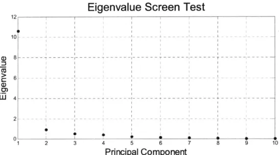
Principal Components Analysis, as described in Section 3 was carried out on the 10 individual datasets using both de-trended and trended volatility. The first result of PCA is the screen test. This is a visual display of the Eigenvalues which enables us to identify their relative importance and how many we should focus on. As an example, Figure 5.1 shows the screen test for the Panamax with 10 rolling quarters using the de-trended volatility.

Eigenvalue Screen Test

12

10 - --- - - -- - - -

--0 0

1 2 3 4 5 6 7 8 9 10

Principal Component

Fig 5.1: Eigenvalue Screen Test for Panamax with De-Trended Volatility

Here we see a sharp decline after the first eigenvalue which means that a single independent statistical factor is very dominant in explaining the variations of this forward curve. Based on this graph, we might decide to focus on the first two or three components since the eigenvalues quickly become insignificant beyond that. In fact, the first

(29)

component alone explains approximately 82% of the volatility while the first 3 explain over 93%.

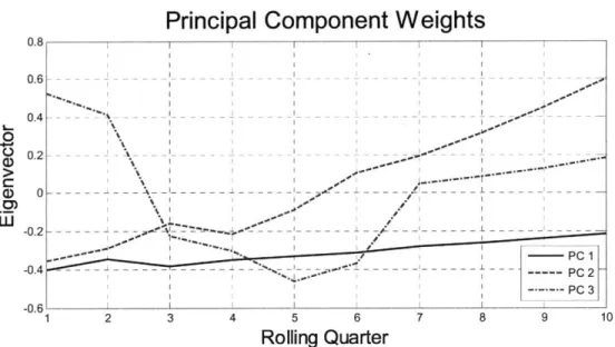
The second result is a plot of the eigenvectors which tells us the weights of the principal components across the various contracts. Figure 5.2 shows the principal component weights of the first three factors for the Panamax with 10 rolling quarters using the de-trended volatility.

Principal Component Weights

1 2 3 4 5 6 7 8 9 10

Rolling Quarter

Fig 5.2: Principal Component Weights for Panamax with De-Trended Volatility

The shapes of the Eigenvector curves indicate how changes or shocks from each factor affect the various contracts and consequently the shape of the forward curve. In this example, we see a different effect by each of the first three principal components:

PC 1: Curve Shift

The first principal component has negative weights for all tenors (the whole curve is negative). This corresponds to a shift of the whole forward curve since a positive shock of the first factor will induce a negative shift in all contracts. The shift is not parallel since the shorter maturity contracts are more volatile and will fluctuate more than the longer maturity contracts.

(30)

PC2: Curve Tilt

The second principal component has negative weights for the short tenors (rolling quarters 1 to 5) and positive weights for the long tenors (rolling quarters 6 to 10). This corresponds to a tilt of the forward curve since a positive shock of the second factor will shift the prompt contracts down and the distant contracts up.

PC3: Change in Curvature

The third principal component has negative weights for the intermediate contracts (rolling quarters 3 to 6) and positive weights for the prompt and distant contracts. This corresponds to a change in the curvature of the forward curve since a positive shock in the third factor will shift short and distant contracts up while shifting intermediate contracts down.

The PCA graphs for the Panamax using de-trended volatility were used here for illustrative purposes. The full set of graphs for all routes using both de-trended and trended volatility can be found in Appendices A and B respectively.

The independent statistical factors described by the eigenvalues and eigenvectors are individual or combinations of real world parameters such as macroeconomic factors that affect the forward curve. This analysis shows us how much volatility is explained by these independent factors. The next step would be to trace relevant macroeconomic factors that are likely to affect the forward curves, and relate them to the independent statistical factors. We can also compare the eigenvectors in highly correlated markets to identify common statistical factors which affect different sectors.

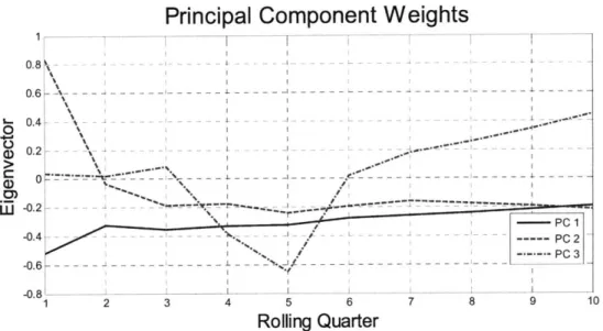
In Section 5.2 we will see that the Panamax and Cape have highly correlated forward curves. Fig 5.3 shows the principal component weights for the Cape with 10 rolling quarters using de-trended volatility. By comparing Fig 5.2 and 5.3, we see that the first and most important principal component has a very similar shape. It corresponds to a negative curve shift with a decreasing impact as contract tenor increases. Further analysis could identify the corresponding real world factor(s) and confirm if it is indeed the same

(31)

for Panamaxes and Capes. If that is the case, one could potentially explain approximately 72% and 82% of the Cape and Panamax forward curve variations just by tracing this factor.

Principal Component Weights

0 . - -- - -- -- - - .-4 % _% 0.6 -\--- - - - - --1 -0.1 2 4 5 6 8 1 0. 4 L - - - - . C P C: 0 --- -- -,\--- --- --- -4 -0.48 C 1 2 3 4 5 6 7 8 9 10 Rolling Quarter

Fig 5.3: Principal Component Weights for Cape with De-Trended Volatility

The cumulative percentage of total volatility explained by the first 5 components was calculated for all routes. The results using de-trended and trended volatility are presented in Tables 5.1 and 5.2 respectively.

PCA Results Using De-Trended Volatility

CAPE PMX CAPE PMX TC-2 TD3 TD5 TC2 TD3 TD5 (22R) (22R) (WS) (WS) (WS) PCI 77.06% 87.65% 71.98% 81.63% 37.39% 46.76% 30.00% 58.04% 67.87% 55.75% PC2 93.26% 93.29% 86.86% 88.76% 52.59% 60.36% 45.92% 78.17% 82.58% 74.42% PC3 96.22% 95.63% 92.42% 93.01% 64.68% 70.93% 58.82% 87.46% 90.08% 85.96% PC4 97.53% 97.19% 95.33% 96.14% 74.29% 79.49% 70.13% 92.31% 94.25% 91.94% PC5 98.48% 98.39% 97.77% 97.91% 83.45% 86.05% 80.61% 95.30% 96.55% 95.20%

Table 5 1 Cuimultive~ Percentage of De--Trended Volatility Explainied by the First 5 Principal Components .k:

(32)

PCA Results Using Trended Volatility CAPE PMX CAPE PMX TC-2 TD3 TD5 TC2 TD3 TD5 (22R) (22R) (WS) (WS) (WS) PC1 99.19% 99.39% 98.99% 99.14% 61.33% 62.25% 48.30% 86.19% 78.31% 75.36% PC2 99.62% 99.66% 99.46% 99.61% 78.39% 74.52% 68.56% 93.71% 88.09% 85.53% PC3 99.78% 99.81% 99.76% 99.84% 88.94% 84.13% 82.92% 97.35% 94.04% 93.45% PC4 99.90% 99.94% 99.88% 99.91% 92.25% 90.10% 88.47% 99.23% 98.24% 98.34% PC5 99.96% 99.96% 99.94% 99.95% 94.82% 94.22% 93.04% 99.70% 99.29% 99.28%

Table 5.2 Cumulative Percentage of Trended Volatility Explained by the First 5 Principal Components

Tables 5.1 and 5.2 tell us how much of the volatility in the forward curve is explained by the dominant independent statistical factors or alternatively, how many independent statistical factors are needed to adequately explain the variations in the forward curve. Unlike for other indices such as electricity prices, Tables 5.1 and 5.2 indicate that only a few principal components are required for the main shipping forward curves. This means that the task of explaining the variations and predicting the forward curves can potentially be simplified to a great extent.

By comparing Tables 5.1 and 5.2 we see that more volatility is explained by the first few factors when using trended volatility as opposed to de-trended volatility. That may be because trend variations may be captured better by a few components than variations about the trend, and these trend variations may account for a significant portion of the total variation.

We also see that more volatility is explained by the first few factors in dry bulk carriers relative to tankers, in datasets of 22 rolling contracts relative to those with 10 rolling contracts, and in those where the analysis has been carried out with prices in Worldscale (WS) as opposed to time charter equivalent (TCE).

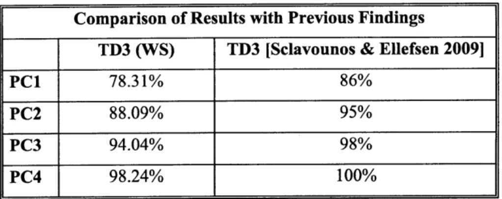
[Sclavounos & Ellefsen 2009] carried out PCA analysis on the TD3 over the period Apr-4-2005 to Feb-6-2009 using monthly rolling futures contracts with tenors ranging from 2 to 5 months. The analysis was carried out using the Worldscale prices and the de-trended measure of volatility. Table 5.3 shows a comparison of our relative results.

(33)

Table 5.3 Comparison of TD3 De-Trended Volatility by First 4 Factors with rSclavounos & Ellefsen 20091

The results of [Sclavounos & Ellefsen 2009] show a higher percentage of volatility explained by the first factor and consequently all the cumulative results are higher. The difference may be partly explained by the fact that in this route, contracts beyond the first few months are significantly less liquid. Our analysis consists of 10 rolling quarters as opposed to rolling months 2 to 5.

Comparison of Results with Previous Findings

TD3 (WS) TD3 [Sclavounos & Ellefsen 2009]

PC1 78.31% 86%

PC2 88.09% 95%

PC3 94.04% 98%

(34)

5.2 Canonical Correlation Results

CCA as described in Section 2 was carried out on the 14 dataset pairs using both de-trended and trended volatility (on a total of 28 block matrices). The main results of CCA are the maximum correlation between the dataset pairs and the corresponding portfolio which achieves the maximum correlation. The maximum correlation by each dataset pair using de-trended and trended volatility is shown in Tables 5.4 and 5.5 respectively.

ROUTES SHIPS UNITS RELATION MAXIMUM

CORRELATION

TD5-TC2 Suezmax - Product $/day Same 99.85%

TD5-TD3 Suezmax - VLCC $/day Same 99.46%

TD3-TC2 VLCC - Product $/day Same 99.17%

CAPE-PMX (22R) Cape - Panamax $/day Same 98.16%

CAPE-PMX Cape - Panamax $/day Same 96.02%

TD5-TD3(ws) Suezmax - VLCC WS Same 84.58%

TD3-TC2(ws) VLCC - Product WS Same 76.95%

TD5-TC2(ws) Suezmax - Product WS Same 75.35%

CAPE-TC2 Cape - Product $/day Cross 28.22%

CAPE-TD5 Cape - Suezmax $/day Cross 27.68%

TD5-PMX Suezmax - Panamax $/day Cross 25.79%

TC2-PMX Product - Panamax $/day Cross 24.91%

TD3-PMX VLCC - Panamax $/day Cross 24.62%

CAPE-TD3 Cape - VLCC $/day Cross 22.10%

Table 5.4: Maximum Correlation of Dataset Pairs Using De-Trended Volatility

The first column contains the names of the dataset pairs which are ranked in both tables by maximum correlation. The second column denotes the two ship types of the

(35)

dataset pair. The data for bulk carriers is always in $/day so the third column is only used to distinguish between the tanker datasets in which the data is in Worldscale and those where the TCE has first been calculated ($/day). Note that the units must always match between the two datasets of a given pair. In the fourth column, if the datasets of the pair are both from tankers or both from bulk carriers, that is indicated by "same". If one is from tankers and the other from bulk carriers, that is denoted as "cross".

For all dataset pairs except "CAPE-PMX (22R)", the data consists of 10 rolling quarters between Feb-10-2005 and Jul-29-2010. For "CAPE-PMX (22R)", the data consists of 22 Rolling quarters between March-10-2008 and July-29-2010.

ROUTES SHIPS UNITS SECTORS MAXIMUM

CORRELATION

TD5-TC2 Suezmax - Product $/day Same 99.96 %

CAPE-PMX (22R) Cape - Panamax $/day Same 99.93 %

TD5-TD3 Suezmax - VLCC $/day Same 99.89%

TD3-TC2 VLCC - Product $/day Same 99.87 %

CAPE-PMX Cape - Panamax $/day Same 99.68 %

TD5-TD3 (WS) Suezmax - VLCC WS Same 98.94 %

TD5-TC2 (WS) Suezmax - Product WS Same 97.52 %

TD3-TC2 (WS) VLCC - Product WS Same 96.83 %

CAPE-TD3 CAPE - VLCC $/day Cross 92.59 %

TD3-PMX Panamax - VLCC $/day Cross 90.90 %

TD5-PMX Panamax - Suezmax $/day Cross 86.42 %

CAPE-TD5 Cape - Suezmax $/day Cross 86.01 %

TC2-PMX Panamax - Product $/day Cross 81.97 %

CAPE-TC2 Cape - Product $/day Cross 81.88 %

Table 5.5: Maximum Correlation of Dataset Pairs Using Trended Volatility

Some general conclusions can be derived by examining and comparing Tables 5.4 and 5.5 as summarized in Table 5.6 and discussed below.

(36)

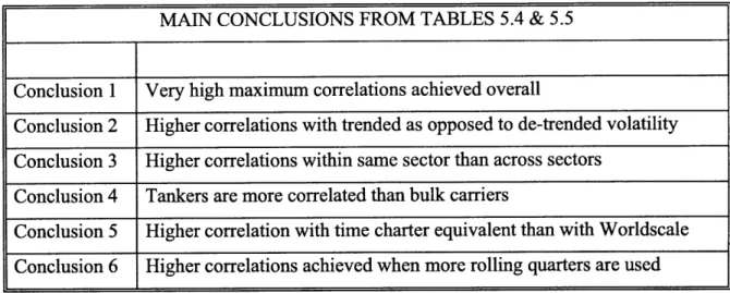
MAIN CONCLUSIONS FROM TABLES 5.4 & 5.5

Conclusion 1 Very high maximum correlations achieved overall

Conclusion 2 Higher correlations with trended as opposed to de-trended volatility Conclusion 3 Higher correlations within same sector than across sectors

Conclusion 4 Tankers are more correlated than bulk carriers

Conclusion 5 Higher correlation with time charter equivalent than with Worldscale Conclusion 6 Higher correlations achieved when more rolling quarters are used

Table 5.6: Summary of Main CCA Conclusions on Maximum Correlation of Dataset Pairs

Conclusion 1.

A surprisingly high maximum correlation can be achieved between most datasets, the highest being 99.96%. This is highlighted when considering the corresponding correlations of the physical (spot) markets. [Stopford 2009] calculates the correlation between average monthly earnings of various major shipping market segments over the period 1990 and 2002.

The comparison with our results may not be perfect because in some instances our chosen routes are not 100% representatives of average earnings, because our analysis uses daily as opposed to monthly time increments, and because we are focusing on different time periods. Nevertheless, the comparison provides a good idea of the relationship between the spot market correlations and maximum possible correlations of the forward curves achieved with CCA.

Note that the relevant results to compare to [Stopford 2009] are only those in $/day (not Worldscale), and those calculated using the trended definition of volatility. Table 5.7 provides a list of the ship type pairs for which we and [Stopford 2009] both have results. They have been ranked by "spot correlation" as calculated by [Stopford 2009]. The fourth column shows our corresponding results from Tables 5.5 for

(37)

comparison with the third column of spot market correlations. The far right column lists the corresponding results from Table 5.4 for illustrative purposes.

ROUTES SHIPS SPOT CANONICAL CANONICAL

CORREL. CORREL. CORREL.

(TRENDED) (DE-TRENDED)

CAPE-PMX (22R) Cape - Panamax 84% 99.93 % 98.16%

CAPE-PMX Cape - Panamax 84% 99.68 % 96.02%

TD3-TC2 VLCC - Product 59% 99.87 % 99.17%

CAPE-TD3 CAPE - VLCC 30% 92.59% 22.10%

CAPE-TC2 Cape - Product 27% 81.88 % 28.22%

TC2-PMX Panamax - Product 17% 81.97% 24.91%

TD3-PMX Panamax - VLCC 7% 90.90 % 24.62%

Table 5.7: CCA Maximum Forward Curve Correlations and Spot Market Correlations by rStopford 20091

Across the 6 ship type pairs, the maximum correlation by CCA using 10 rolling quarters, is on average higher than the correlation of the physical (spot) markets, by 54% when using trended volatility and by 12% when using de-trended volatility.

Conclusion 2.

A higher correlation is achieved between the same dataset pairs when using trended volatility than when using de-trended volatility. This is evident by comparing the results of Table 5.4 (de-trended) with the corresponding results of Table 5.5 (trended). The maximum correlation when using trended as opposed to de-trended volatility is higher in all 14 dataset pairs. The range of correlations jumps from 22.1% - 99.85% to

81.88% -99.96%.

Table 5.8 groups the various dataset pairs according to sector, data units and number of rolling quarters (all are 10 except when noted as "22R"). It then gives the

(38)

average maximum correlation within each group when calculated using de-trended and trended volatility.

Group of Database Pairs Average Max Correlation Average Max Correlation (De-Trended Volatility) (Trended Volatility)

Tanker-Tanker (TCE) 99.50% 99.91%

Bulk-Bulk (22 R) 98.16% 99.93%

Bulk-Bulk 96.02% 99.68%

Tanker-Tanker (WS) 78.96% 97.76%

Bulk-Tanker 25.56% 86.63%

Table 5.8: Maximum Correlation of Dataset Pairs Using Trended Volatility

Here we see the same result again. However, focusing on the bottom two rows, we also notice that the difference is significantly greater when doing the analysis in Worldscale and particularly when correlating across sectors (tankers with bulk carriers).

We can attempt to explain this by recalling the wave analogy of trended and de-trended volatility. The long wave is captured only by the de-trended volatility whereas the de-trended volatility only looks at the short waves riding the long wave. The fact that higher correlations are consistently achieved with trended volatility is a strong indication that the trends may be strongly correlated.

It seems that when comparing across sectors (tankers with bulk carriers), a significant part of the correlation is in the trends and is only captured when looking at the long wave. For example, CCA with trended volatility may better capture the effects of global economic factors such as the sub-prime crisis which sends the whole economy (both sectors) on a downward trend. CCA with de-trended volatility, on the other hand, may be impacted more by "daily" sector-specific factors such as an oil price spike or an iron ore port congestion which only impacts one of the two sectors and hence reduces the overall correlation.

(39)

Conclusion 3.

Higher maximum correlations are achieved when the ship types in the dataset pair are either both tankers or both bulk carriers, than if there is one from each. That is because intuitively, there is a higher earnings correlation between any two tanker or bulk carrier routes or sizes since they are serving similar markets. When comparing the Cape market (mainly 170,000t batches of iron ore and coal), with that of the TC2 (37,000t batches of clean products such as gasoline), there is relatively little in common and they respond to different shocks. In Table 5.7 we see that also spot market correlations by [Stopford 2009] are higher within the same sectors relative to correlations of tanker-bulk carrier pairs.

Conclusion 4.

Tankers are more correlated than bulk carriers. Note that we must only consider pairs with 10 rolling quarters for consistency in this comparison. The results may be explained by the fact that tankers carry more similar cargos. VLCCs and Suezmaxes for example both transport crude oil while the market for transportation of clean products may also be closely linked. Panamaxes on the other hand transport much more grain and also other cargos besides iron ore and coal which are the predominant Cape cargos.

Conclusion 5.

A higher correlation is achieved between the tanker routes when the analysis is performed using $/day as opposed to Worldscale, in other words after the TCE has been calculated. That is simply because by converting to TCE, the noise due to the annual flat-rate changes is eliminated. The futures prices in $/day are more reflective of reality because our assumption that the applicable flat rate was known in advance at the time of the contract is not a bad one to make.

(40)

Conclusion 6.

The last conclusion is that the maximum correlation increases when we add more contracts. Even though a shorter time period is considered, the maximum correlation between the Cape and Panamax is significantly higher with 22 rolling quarters than with 10 rolling quarters. This is true when using both trended and de-trended volatility. The reason is that a larger portfolio of assets (22 as opposed to 10 in each portfolio) provides much more flexibility. One should note that the range of solutions when using fewer rolling quarters is a subset of the range of solutions with more rolling quarters, so the maximum correlation can only increase by adding contracts.

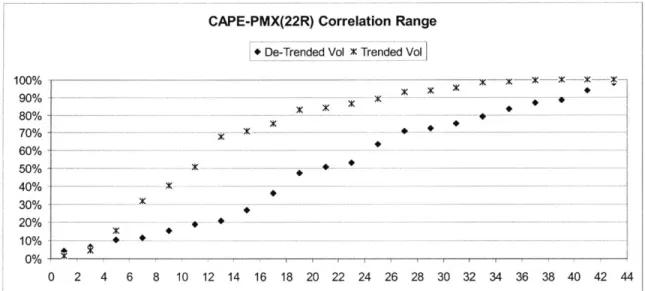
Another interesting result is the minimum correlation attainable within each dataset or the range of possible correlations. While one may want to maximize the correlation for hedging or trading purposes, one may also be interested in minimizing the correlation for diversification. The real positive eigenvalues of the covariance matrix indicate possible correlations that can be achieved between the two datasets. Fig 5.4

shows the possible correlations between the Cape and Panamax forward curves using 22 rolling quarters with de-trended and trended volatility.

CAPE-PMX(22R) Correlation Range + De-Trended Vol X Trended Vol

100% - A - --90% - - - -K--80% - -70% - -)K 60% 50% -40% -30% -20% 10% 0 2 4 6 8 10 12 14 16 18 20 22 24 26 28 30 32 34 36 38 40 42 44