HAL Id: hal-00936745
https://hal.inria.fr/hal-00936745
Submitted on 27 Jan 2014
HAL is a multi-disciplinary open access
archive for the deposit and dissemination of
sci-entific research documents, whether they are
pub-lished or not. The documents may come from
teaching and research institutions in France or
L’archive ouverte pluridisciplinaire HAL, est
destinée au dépôt et à la diffusion de documents
scientifiques de niveau recherche, publiés ou non,
émanant des établissements d’enseignement et de
recherche français ou étrangers, des laboratoires
Elimination
David Coudert, Alvinice Kodjo, Khoa Phan
To cite this version:
David Coudert, Alvinice Kodjo, Khoa Phan. Robust Energy-aware Routing with Redundancy
Elimi-nation. [Research Report] RR-8457, INRIA. 2014. �hal-00936745�
0249-6399 ISRN INRIA/RR--8457--FR+ENG
RESEARCH
REPORT
N° 8457
January 2014Robust Energy-aware
Routing with
Redundancy Elimination
RESEARCH CENTRE
SOPHIA ANTIPOLIS – MÉDITERRANÉE
Redundancy Elimination
David Coudert
∗ †, Alvinice Kodjo
† ∗, T. Khoa Phan
† ∗Project-Teams COATI
Research Report n° 8457 — January 2014 — 22 pages
Abstract: Many studies in literature have shown that energy-aware routing (EAR) can sig-nificantly reduce energy consumption for backbone networks. Also, as an arising concern in net-working research area, the protocol-independent traffic redundancy elimination (RE) technique helps to reduce (a.k.a compress) traffic load on backbone network. Motivation from a formulation perspective, we first present an extended model of the classical multi-commodity flow problem with compressible flows. Moreover, our model is robust with fluctuation of traffic demand and compression rate. In details, we allow any set of a predefined size of traffic flows to deviate simul-taneously from their nominal volumes or compression rates. As an applicable example, we use this model to combine redundancy elimination and energy-aware routing to increase energy efficiency for a backbone network. Using this extra knowledge on the dynamics of the traffic pattern, we are able to significantly increase energy efficiency for the network. We formally define the problem and model it as a Mixed Integer Linear Program (MILP). We then propose an efficient heuristic algorithm that is suitable for large networks. Simulation results with real traffic traces on Abilene, Geant and Germany50 networks show that our approach allows for 16 − 28% extra energy savings with respect to the classical EAR model.
Key-words: Robust Network Optimization, Green Networking, Energy-aware Routing, Redun-dancy Elimination
This work has been partially supported by Région PACA.
∗Inria, France
Elimination
Résumé : La gestion efficace de la consommation de l’énergie des réseaux de télécommuni-cations est de nos jours un sujet d’une très grande importance. Plusieurs études ont réussi à prouver que le routage basé sur la consommation d’énergie réduit considérablement la consom-mation totale d’énergie du réseau. Nous avons dans cet article, combiné cette technique à celle de l’élimination de redondance de trafic, pour diminuer davantage l’energie consommée par un réseau coeur. Nous avons considéré une formulation robuste de ce problème dans le cas où il existe une incertitude autant au niveau de la valeur du volume de trafic que de celui du traux de redondance. Nous proposons, pour résoudre ce problème, un modèle linéaire, un algorithme exacte et une heuristique qui nous permettent des économies d’énergie allant de 16% à 28% comparé à la méthode classique de routage baseé sur l’énergie.
Mots-clés : Robust Network Optimization, Green Networking, Energy-aware Routing, Re-dundancy Elimination
1
Introduction
Recent studies have shown that ICT is responsible for 2% to 10% of the worldwide power con-sumption [1, 2]. For example, the Global e-Sustainability Initiative estimated the overall network energy requirement for European telecommunication is around 35.8 TWh in 2020 [3]. To this extend, the backbone networks and more precisely IP routers, consume a majority of energy [4]. While the traffic load has only a marginal influence, the most contribution of energy consumption on router is the number of active elements such as ports, line cards, base chassis [5]. Traditionally, networks are always designed to meet the peak-hour traffic demand. Therefore during normal periods, the traffic load is typically well below the network capacity. Following this observation, people have proposed energy-aware routing (EAR) approach aiming at minimizing the number of used links while all the traffic demands are routed without any overloaded links [2, 6, 7].
Another research topic that has also been active recently is traffic redundancy elimination (RE) [8, 9, 10, 11, 12]. Observing that traffic on the Internet contains a large fraction of re-dundancy (e.g. popular contents such as new movies are often downloaded several times sub-sequently), a complementary approach uses redundancy elimination (RE) techniques to reduce link load in backbone networks. It consists in splitting packets into small chunks, each is indexed with a small key, that are cached along traffic flows as long as they are popular. Then, keys are substituted to chunks in traffic flows to avoid sending multiple times the same content, and the original data are recovered on downstream routers based on the cache synchronization be-tween the sending and the receiving routers. Therefore, traffic redundancy is removed and traffic volumes of flows between the two routers are reduced. For simplicity, a traffic flow from which redundancy has been removed is called a compressed flow. We use interchangeably the notation compression rate or RE rate to denote how much traffic redundancy can be eliminated.
From energy savings perspective, RE has a drawback since it increases energy consumption of routers [13]. To find a good trade-off, in our previous work, we proposed GreenRE - a model that combines EAR and RE to increase energy efficiency for backbone network [13]. In the GreenRE model, each of the demand has a static traffic volume and is associated with a constant factor of redundant traffic. To handle future changes and guarantee a certain level of quality of service (QoS) (avoiding overloaded links), the peak volumes of traffic demand and the lowest RE rates are used as the worst case realization. Such assumption clearly leads to inefficient usage of network resources and poor energy savings. To alleviate this limitation of the GreenRE model, the uncertainty on traffic volumes and RE rates has to be precisely modeled and taken into account in the optimization process. By using this extra information, we are able to obtain a design that is more closely related to the dynamics of the traffic pattern, hence significantly increase energy savings compared to previous proposals.
In mathematical literature, the technology-independent Γ-robustness has been introduced in [14, 15] and then successfully applied to various network design problems [16, 17, 18, 19]. This approach is based on an observation that in real traffic traces, only a few of the demands are simultaneously at their peaks. So, the authors considered a parameter Γ > 0 so that at most Γ demands deviate simultaneously from their nominal traffic volumes. Based on this assumption, the so-called robust solution is a solution that is feasible for any subset of Γ demands simulta-neously at their peaks, other demands are being at their nominal values. The originality of the method is the expression of the maximum sum of deviation over all possible subsets of Γ demands as a unique linear program (LP). However, this LP formulation may have an exponential number of constraints. To overcome this issue, the LP formulation is transformed into a compact one using the duality theorem.
In this work, we first present an extended version of the classical multi-commodity flow problem in which traffic flows can be compressed to smaller volumes (with some certain costs,
e.g. energy cost mentioned in this paper). In addition, we show that the robustness combining uncertainties in both traffic demand and compression rate is very challenging. In summary, we make the following contributions:
• From a theoretical point of view, we present an extended multi-commodity flow problem with compressible traffic flows. In addition, we provide a complete picture in which uncer-tainties in both traffic volumes and compression rates are taken into consideration. • This extended model can be applied to a vast range of applications in network flows and
traffic management. In this paper, as an applicable example, we use this model to increase energy efficiency for a backbone network. We apply this extended model into energy-aware routing and formally define the Robust-GreenRE problem using mixed integer linear program (MILP).
• Since robust network design is NP-hard problem [20], we propose a heuristic algorithm that is effective for large instances.
• By simulation, we show the energy savings offered by our methods on backbone networks with real-life data traffic traces and compression rate fluctuations.
2
Related Works
2.1
Energy-aware Routing (EAR)
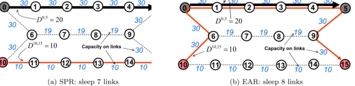
0 6 7 8 10 9 30 30 30 30 30 19 19 19 30 10 10 10 10 10 5 15 30 30 30 Capacity on links 1 2 3 4 11 12 13 14 0,5 20 D = 10,15 10 D =
(a) SPR: sleep 7 links
6 7 8 10 9 11 12 13 14 30 30 30 30 30 19 19 19 30 10 10 10 10 10 5 15 30 30 30 Capacity on links 0 1 2 3 4 0,5 20 D = 10,15 10 D =
(b) EAR: sleep 8 links
Figure 1: Example of Shortest path routing (SPR) vs. energy-aware routing (EAR) As an example of EAR, we refer to Fig. 1. There are two traffic demands 0 → 5 and 10 → 15 with volumes D0,5 = 20 Gbps and D10,15 = 10 Gbps. The shortest path routing, as shown in
Fig. 1a, uses 10 active links whereas the remaining 7 links can be put into sleep mode. However, taking energy consumption into account, in Fig. 1b, EAR solution allows to put 8 links into sleep mode, thus energy consumption is further decreased. The problem of minimizing the number of active links under QoS constraints can be precisely formulated using MILP. However, this problem is known to be NP-Hard [21], and currently exact solutions can only be found for small networks. Therefore, many heuristic algorithms have been proposed to find admissible solutions for large networks [21, 2].
2.2
Redundancy Elimination
Internet traffic exhibits a large amount of redundancy when different users access the same or similar contents. Therefore, several works [22, 8, 9, 23, 10, 11] have explored how to eliminate
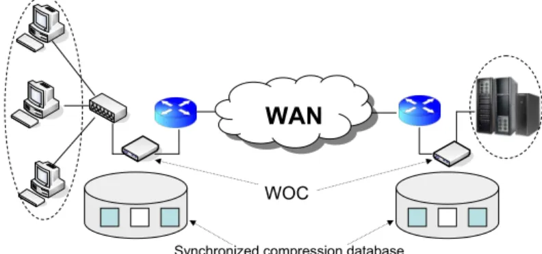
traffic redundancy on the network. Spring et al. [22] developed the first system to remove redundant bytes from any traffic flows. Following this approach, several commercial vendors have introduced Wide area network Optimization Controller (WOC) - a device that can remove duplicate content from network transfers [24, 25, 26]. WOCs are installed at individual sites of small Internet Service Providers (ISPs) or enterprises to offer end-to-end RE between pairs of sites. As shown in Fig. 2, the patterns of previously sent data are stored into the databases of
WAN
` WOC
Synchronized compression database
Figure 2: Reduction of end-to-end link load using WOC
the WOCs at both sending and receiving sides. The technique used to synchronize the databases at peering WOCs can be found in [25]. Whenever the WOC at the sending side notices the same data pattern coming from the sending hosts, it substitutes the original data with a small signature (encoding process). The receiving WOC then recovers the original data by looking up the signature in its database (decoding process). Because signatures are only a few bytes in size, sending signatures instead of actual data gives significant bandwidth savings.
Recently, the success of WOC deployment has motivated researchers to explore the benefits of deploying RE in routers across the entire Internet [8, 9, 23, 10]. The core techniques used here are similar to those used by the WOC: each router on the network has a local cache to store previously sent data used to encode and decode data packets later on. Obviously, this technique requires heavy computation and large memory for the local cache. However, Anand et al. [23] have shown that on a desktop equipped with a 2.4 GHz CPU and 1 GB RAM, the prototype can work at 2.2 Gbps for encoding and at 10 Gbps for decoding packets . Moreover, they believe that higher throughput can be obtained if the prototype is implemented in hardware. Several real traffic traces have been collected to show that up to 50% of the traffic load can be reduced with RE support [9, 23, 10].
In next sub-section, we recall the GreenRE model - the first model of energy-aware routing with RE support [13]. Although RE was initially designed for bandwidth savings, it is also interesting for reducing the network power consumption.
2.3
GreenRE - Energy Savings with Redundancy Elimination
In the GreenRE model, RE is used to virtually increase capacity of the network links. A drawback is that, as shown in [13], when a router performs RE, it consumes more energy than usual. This introduces a tradeoff between enabling RE on routers and putting links into sleep mode. We show that it is a non-trivial task to find which routers should perform RE and which links should sleep to minimize energy consumption for a backbone network.
2.3.1 Example of GreenRE model 0 1 2 3 4 10 11 12 13 14 30 30 30 30 30 19 19 19 30 10 10 10 10 10 5 15 30 30 30 Capacity on links RE-router 6 7 8 9 RE-router 0,5 20 D = 10,15 10 D = 10,15 10 D = 0,5 20 D = 0,5 10 comp D = +ε 10,15 5 ' comp D = +ε
(a) 10 links in sleep mode, 2 enabled RE-routers
0 1 2 3 4 10 11 12 13 14 30 30 30 30 30 19 19 19 30 10 10 10 10 10 5 15 30 30 30 Capacity on links RE-router 6 7 8 9 RE-router 0,5 20 D = 10,15 10 D = 10,15 10 D = 0,5 20 D = 0,1 20 D = 0,5 10 comp D = +ε 10,15 5 ' comp D = +ε
(b) 9 links in sleep mode, 2 enabled RE-routers Figure 3: GreenRE with 50% of traffic redundancy
The example presented in Fig. 3a has two traffic demands D0,5 = 20 Gbps and D10,15 = 10
Gbps. Let a RE-router consume 30 Watts [13] and a link consume 200 Watts [2]. Assume that 50% of the traffic is redundant and RE service is enabled at routers 6 and 9, thus the traffic flows 0 → 5 and 10 → 15 passing through links (6, 7, 8, 9) are reduced to 10 Gbps and 5 Gbps, respectively. Therefore the routing in Fig. 3a is feasible without any congestion. As a result, the GreenRE solution allows to put 10 links in sleep mode and to enable 2 RE-routers which saves (10 × 200 − 2 × 30) = 1940 Watts, compared to the saving of 8 × 200 = 1600 Watts of the EAR solution (Fig. 1b). It is noted that, in some extreme cases, GreenRE even helps to find feasible routing solution meanwhile it is impossible for the classical EAR. For example, if we add a third demand from router 0 to router 1 with volume 20 Gbps, then Fig. 3b is a feasible solution. However, without RE-routers, no feasible solution is found because there is not enough capacity to route all the three demands.
2.3.2 Problem Formulation
We consider a communication backbone network where nodes represent routers with multiple in-terfaces that are used to create physical links. The GreenRE problem is defined on an undirected graph G = (V, E) where V is a set of routers and E represents a set of links. In this network, any physical link between two routers is a bi-directional link, one direction is for the down-stream and the opposite direction is for the up-stream. We use the notation{uv} to denote a physical link (without direction) and uv as an arc with direction from u to v. A link {uv} is considered to be active if there is data going through at least one of its directions. Each active link{uv} and router u is respectively associated with a power consumption value P E{uv}= 200 Watts [2] and P Nu = 30 Watts [13]. We are given a set D = {(s, t) ∈ V × V : s ̸= t} representing the traffic
percent-age of traffic redundancy of the demand (s, t). Corresponding to λst, we define γst= (1 − λst)
which represents the percentage of unique (non redundant) traffic. For instance, for a 10 Gbps traffic demand with λst = 40% of redundancy, its volume can be reduced by RE technique to
10 × γst= 6 Gbps of non-redundant traffic. For simplicity, a traffic flow from which redundancy
has been removed is called a compressed flow.
We use binary variables x{uv}and wu to denote respectively activated links and RE-routers.
N (u) is the set of neighbors of u in the graph G. Variables fst
uv and guvst, ∀{uv} ∈ E, (s, t) ∈ D
denote the fraction of normal and compressed flows (s, t) on link (u, v). We reformulate the GreenRE model as follows:
min ∑ {uv}∈E P E{uv}x{uv}+∑ u∈V P Nuwu (1) s.t. ∑ v∈N(u) ( fst vu+ gvust − fuvst − guvst ) = −1 if u = s, 1 if u = t, 0 otherwise ∀u ∈ V, (s, t) ∈ D (2) ∑ (s,t)∈D Dst(fst uv+ γstguvst ) ≤ µCuvx{uv} ∀{uv} ∈ E (3) ∑ v∈N(u) ( gst uv− gvust ) ≤ wu ∀u ∈ V, (s, t) ∈ D (4) ∑ v∈N(u) ( gstvu− guvst ) ≤ wu ∀u ∈ V, (s, t) ∈ D (5) 0 ≤ fst uv, guvst ≤ 1 ∀(u, v) ∈ E, (s, t) ∈ D (6) x{uv}, wu∈ {0, 1} ∀{uv} ∈ E, u ∈ V (7)
The objective function (1) is to minimize the power consumption of the network represented by the number of active links and activated RE-routers. Constraints (2) establish flow conser-vation constraints when considering simultaneously the normal (fst
uv) and the compressed (guvst)
flows. Note that both the normal and compressed flows can be fractional. The constraints (2) indicate that the sum of flows entering in a router is equal to the sum of flows outgoing from it except if the router is either the source or the destination of the demand. For example, suppose that a normal flow fst
vu enters in a router u and leaves it with 50% of compressed flow, then we
have fst
vu = 1, gstvu = 0, fuvst = 0.5 and gstuv = 0.5 making thus the difference equal to 0. We
use constraints (3), where µ denotes the link utilization in percentage, to limit the available capacity of a link. Constraints (4) and (5) are used to determine whether RE service is enabled on router u or not. If it is not (wu= 0), the router u only forwards flows without compression
or de-compression, then the amount of compressed flows incoming and outgoing the router u is unchanged. It is noted that if a flow is compressed, it needs to be decompressed somewhere on the way to its destination. This requirement is implicitly embedded in the constraints (5). For instance, assume that a destination node t is not a RE-router (wt= 0). When a compressed flow
gst
vt reaches its destination, because t is the last node on its path, the flow can not be
decom-pressed. Consider the constraints (5), we have u = t, then∑v∈N(u)gst
vt> 0 (the compressed flow
enters node t) and∑v∈N(u)gst
tv = 0 (t is the destination node). Therefore, the constraint (5) is
violated and the flow should be decompressed before or at least at the destination node (wt= 1).
Although the GreenRE model is already a complex task, it does not take the fluctuation in real-life traffic into account. In practice, the actual traffic demand Dst and the redundant
proposed to address this issue by taking both traffic demand and redundancy rate uncertainty into account while satisfying the capacity constraints (3).
2.4
Robust Optimization
Over the past years, robust optimization has been established as a special branch of mathematical optimization allowing to handle uncertain data [27, 28]. A specialization of robust optimization, which is particularly attractive by its computational tractability, is the so-called Γ-robustness concept introduced by Bertsimas and Sim [14, 15]. Instead of deterministic coefficients, the coefficients aj of a constraint ∑jajxj ≤ b are assumed to be random variables. Bertsimas
and Sim have shown that in case all random variables are independent and have a symmetric distribution of the form aj ∈ [¯aj − ˆaj, ¯aj + ˆaj] (with ¯aj the average and ˆaj the maximum
deviation), it can be guaranteed that the constraint is satisfied with high probability by defining an appropriate integer Γ and replacing the constraint by
∑ j ¯ ajxj+ max J:|J|≤Γ ∑ j∈J ˆ ajxj ≤ b. (8)
This constraint models that, for each realization of the uncertainties, at most Γ many (but arbitrary) coefficients can deviate from their nominal value. Given an arbitrary realization, it is shown in [14, 15], that the probability that (8) is violated, is about 1 − Φ(Γ−1√
n), where Φ is the
cumulative distribution function of the standard normal distribution and n equals the number of uncertain coefficients. This result is independent of the actual distribution of aj.
Note that constraint (8) is deterministic and the complete problem can be reformulated as a standard mixed integer problem. So the model including uncertainty can be solved by the same means as the original problem. Again see [14, 15] for details. From a practical perspective, by varying the parameter Γ, different solutions can be obtained with different levels of robustness (the higher Γ the more robust, but also the more expensive the solution is). This concept has already been applied to several network optimization problems [29, 16, 30].
3
Robust-GreenRE Model
Fig. 4 shows real traffic traces of the three source-destination pairs: (a)Washington D.C. - Los Angeles, (b) Seattle - Indianapolis, and (c) Seattle - Chicago in the US Abilene Internet2 network in intervals of 5 mins during the first 10 days of July 2004 [17]. We observe that, at some points, each traffic demand can achieve a maximum (peak) value. However, the traffic peaks do not occur simultaneously for the three demands. This confirms an assumption that the number of simultaneous demand peaks is bounded [17]. Hence, we propose in this section a Robust-GreenRE model to deal with this kind of uncertainty.
In the Robust-GreenRE model, two values determining percentage of non-redundant traffic are given for each traffic demand: a nominal (default) value γst∈ (0, 1] and a deviation bγstsuch
that 0 ≤ bγst, γst+bγst≤ 1 and the actual non-redundant rate γst ∈ [γst, γst+bγst]. Similarly, each
traffic demand is given by a nominal value Dst≥ 0 and a deviation bDst≥ 0 so that the actual
demand volume Dst ∈ [Dst, Dst+ bDst]. Potentially, each demand is expressed with its default
value: Dst= Dstand Dst
comp= γst×D st
. In the worst case realization, the peak values should be used and each traffic pair is expressed by Dst= (Dst+ bDst) and Dst
comp= (γst+bγst)×(D st
+ bDst).
Given two integral parameters 0 ≤ Γd, Γγ ≤ |D| (|D| is the total number of demands), we denote
Peak traffic Peak traffic Peak traffic (a) (b) (c)
Figure 4: Traffic demands in Abilene network [17]
volumes. Similarly, Q′ ⊆ D, |Q′| ≤ Γ
γ, is a set of demands in which all RE rates can deviate
simultaneously. Observe that demands in Q ∩ Q′ are simultaneously at their peak traffic and
lowest RE rates. Given (Γd, Γγ) as the desired robustness of the network, the Robust-GreenRE
problem is to minimize the energy consumption of the network while satisfying the link capacity constraints whenever at most Γd demands and Γγ RE rates deviate simultaneously from their
nominal values.
Table 1: Demands and redundancy rates variation Demand (s, t) Dst Dbst γst
bγst
(0, 3) 3 1 0.5 0.3
(4, 7) 2 1 0.6 0.3
(8, 11) 1 2 0.7 0.3
Let us analyze the example of Fig. 5 to see that it is non-trivial to solve the Robust-GreenRE problem. We consider a (3 × 4) grid with a capacity of 4 Mbps per direction of each links. There are three traffic demands to be routed: (0, 3), (4, 7) and (8, 11), each with respective nominal traffic volumes Dst and deviation bDst (resp. nominal RE rates γst and deviation bγst) as shown
in Table 1. As shown in Fig. 5a, this is the optimal solution for the case in which no uncertainty is defined (Γd= Γγ = 0). In this solution, we activate two RE-routers at nodes 4 and 7 and the
total traffic passing through links (4−5−6−7) is equal to D0,3×γ0,3+D4,7×γ4,7+D8,11×γ8,11 =
3 × 0.5 + 2 × 0.6 + 1 × 0.7 = 3.4 < 4.
Consider now the robust case in which Γd = Γγ = 1. There are 9 possible cases for the
combinations of deviation in traffic volumes and RE rate as reported in Table 2. In Case 1, demand (0, 3) deviates both on its traffic volume and RE rate. Thus the solution of Fig. 5a is infeasible because the traffic volume passing through links (4 − 5 − 6 − 7) is (D0,3 + bD0,3) ×
(γ0,3+ bγ0,3) + D4,7× γ4,7+ D8,11× γ8,11 = (3 + 1) × (0.5 + 0.3) + 2 × 0.6 + 1 × 0.7 = 5.1 > 4.
The optimal solution in this case is presented in Fig. 5b in which 8 links are actived and no RE-router is used. The power consumption is 8 × 200 = 1600 Watts. In Case 9, both the traffic volume and the RE rate of demand (8, 11) deviate simultaneously. The solution in Fig. 5b is infeasible in this case even if we enable RE-routers at node 4 and 7 since the total traffic passing through links (4 − 5 − 6 − 7) will be D4,7 × γ4,7+ (D8,11+ bD8,11) × (γ8,11+ bγ8,11) =
2 × 0.6 + (1 + 2) × (0.7 + 0.3) = 4.2 > 4. In Case 9, the optimal solution is the one of Fig. 5c with 8 active links and 2 RE-routers. However, in the Robust-GreenRE model with Γd= Γγ = 1, any
a. 7 active links and 2 RE-routers 0 10 5 1 2 3 11 6 8 9 0 10 5 1 2 3 4 11 6 7 8 9 4 7 RE-router RE-router 10 5 1 2 4 11 6 7 8 9
b. 8 active links and 0 RE-router
c. 8 active links and 2 RE-router
0 10 5 1 2 3 4 11 6 7 8 9
d. 9 active links and 0 RE-router
0 3
RE-router RE-router
Figure 5: Example of robustness Table 2: 9 cases of the robustness
Case Q Q’ Best solution Link load luv(Mbps)
1 (0,3) (0,3) Fig. 1b l0,1,2,3= 4, l4,5,6,7= 3, (1600 Watts) l8,4= l7,11= 1 2 (0,3) (4,7) (1600 Watts)Fig. 1b l0,1,2,3l = 4, l4,5,6,7= 3, 8,4= l7,11= 1 3 (0,3) (8,11) Fig. 1b l0,1,2,3= 4, l4,5,6,7= 3, (1600 Watts) l8,4= l7,11= 1 4 (4,7) (0,3) Fig. 1b l0,1,2,3= 3, l4,5,6,7= 4, (1600 Watts) l8,4= l7,11= 1 5 (4,7) (4,7) Fig. 1b l0,1,2,3= 3, l4,5,6,7= 4, (1600 Watts) l8,4= l7,11= 1 6 (4,7) (8,11) Fig. 1b l0,1,2,3= 3, l4,5,6,7= 4, (1600 Watts) l8,4= l7,11= 1 7 (8,11) (0,3) Fig. 1c l0,1,2,3= 3.6, l4,0= 2, (1660 Watts) l8,9,10,11= 3, l3,7= 2 8 (8,11) (4,7) Fig. 1c l0,1,2,3= 3.3, l4,0= 2, (1660 Watts) l8,9,10,11= 3, l3,7= 2 9 (8,11) (8,11) Fig. 1c l0,1,2,3= 2.7, l4,0= 2, (1660 Watts) l8,9,10,11= 3, l3,7= 2
demand can deviate from its nominal volume or RE rate, as long as at most one demand and one RE rate deviate their volumes at the same time. Consequently, a solution is feasible if and only if it satisfies all of the 9 cases. Hence, Fig. 5d is the only feasible solution since Fig. 5c is infeasible for Case 1 of Table 2.
The idea of robustness is that we should reserve some space in the link capacity to accom-modate the fluctuation in the traffic volumes and RE rates. To do so, we define a function δ(f, g, Γd, Γγ) such that the capacity constraints satisfy:
∑
(s,t)∈D
Dst(fuvst + γstgstuv
)
+ δ(f, g, Γd, Γγ) ≤ µCuvxuv (3’)
The problem now is to find the value of the function δ(f, g, Γd, Γγ). To answer this question,
Qdγ contains demands in which both traffic volumes and RE rates can deviate, Qd (resp. Qγ)
contains demands in which only traffic volumes (resp. RE rates) can deviate from their nominal values. Actually, we can formulate the problem using the two sets Q (demands variation) and Q′ (RE rates variation). However, it will result in a non-linear formulation. For simplicity, we
use the notation e instead of uv, ∀ {uv} ∈ E. Then the worst case scenario when considering fluctuation on an arc e is given by:
∑ (s,t)∈D Dstfst e + max Q⊆D { ∑ (s,t)∈Q b Dstfst e } + ∑ (s,t)∈D Dstγstgst e + max Qγ=Q′\Q { ∑ (s,t)∈Qγ Dstbγstgst e } + max Qdγ=Q∩Q′ { ∑ (s,t)∈Qdγ ( bDstbγst+ bDstγst+Dstbγst)gst e } + max Qd=Q\Q′ { ∑ (s,t)∈Qd b Dstγstgst e } ≤ µCexe (3”) Obviously, Constraints (3’) and (3”) are equivalent if δ(f, g, Γd, Γγ) is the maximum part of
Constraint (3”). Constraint (3”) can be rewritten as a set of many constraints corresponding to all possible sets Qd, Qγ and Qdγ, but the resulting model has an exponential number of
constraints. We thus propose three methods to overcome this difficulty.
3.1
Compact formulation
Given fst
e , gest, Γd, and Γγ, the function δ(f, g, Γd, Γγ) can be computed by:
(primal) δ(f, g, Γd, Γγ) = max ∑ (s,t)∈D ( b Dstfest(ze,Qst d+z st e,Qdγ)+D st bγstgestze,Qst γ+( bD st bγst+ bDstγst+Dstbγst)gsteze,Qst dγ+ bD stγstgst eze,Qst d ) s.t. ∑ (s,t)∈D ( zst e,Qd+ z st e,Qdγ )
≤ Γd ∀e ∈ E [πe,d] (3a)
∑
(s,t)∈D
(zst e,Qγ+ z
st
e,Qdγ) ≤ Γγ ∀e ∈ E [πe,γ] (3b)
ze,Qst d+ z st e,Qdγ+ z st e,Qγ≤ 1 ∀e ∈ E, (s, t) ∈ D [σ st e] (3c) zst e,Qd∈ {0, 1} ∀e ∈ E [ρ st e,d] (3d) zst e,Qγ∈ {0, 1} ∀e ∈ E [ρ st e,γ] (3e) zst e,Qdγ ∈ {0, 1} ∀e ∈ E [ρ st e,dγ] (3f)
where binary variables zst e,Qd, z
st
e,Qγ and z
st
e,Qdγ denote whether a traffic pair (s, t) belongs respec-tively to the sets Qd, Qγ, Qdγ or not. Note that, a traffic demand (s, t) can belong exactly to
one and only one of the three sets Qd, Qγ and Qdγ. Constraints (3a) and (3b) are used to limit
size of the set|Q| = |Qd∪ Qdγ| ≤ Γd and|Q′| = |Qγ∪ Qdγ| ≤ Γγ. Constraint (3c) indicates that
no traffic pair (s, t) can belong to more than one of the three sets Qd, Qγ and Qdγ.
We now need to find LP duality of the above primal problem using dual variables πe,d, πe,γ,
σst
e, ρste,d, ρste,dγ and ρste,γ. To do so, we first relax the last three constraints (3d), (3e) and (3f) to
real variables: 0 ≤ zst e,Qd, z
st e,Qdγ, z
st
e,Qγ ≤ 1. By employing LP duality for the relaxation of the primal, we obtain:
(dual) δrelax(f, g, Γd, Γγ) = min Γdπe,d+ Γγπe,γ+
∑
(s,t)∈D
(σst
s.t. πe,d+ σste + ρste,d≥ bDst(fest+ γstgest) ∀(s, t) ∈ D (3a’)
πe,d+ πe,γ+ σste + ρste,dγ≥ bDstfest+
( b Dstbγst+ bDstγst+ Dstbγst)gst e ∀(s, t) ∈ D (3b’) πe,γ+ σste + ρste,γ ≥ D st bγstgst e ∀(s, t) ∈ D (3c’)
πe,d, πe,γ, σest, ρe,dst , ρste,γ, ρste,dγ≥ 0 ∀(s, t) ∈ D (3d’)
Since the primal problem is a max problem, the optimal value of the relaxation of the primal δrelax(f, g, Γd, Γγ) is greater or equal to the original one δ(f, g, Γd, Γγ). As a result, the objective
of the duality of the relaxation is also greater or equal to δ(f, g, Γd, Γγ) and it makes the capacity
constraint strongly robust. By embedding this duality of the relaxation into (1)–(7), the (strong) Robust-GreenRE problem can be compactly formulated by replacing Constraint (3) with:
∑
(s,t)∈D
(σst
e + ρste,d+ ρste,γ + ρste,dγ) +
∑
(s,t)∈D
Dst(fst
e + γstgste) + Γdπe,d+ Γγπe,γ ≤ µCexe ∀e ∈ E
and adding constraints (3a’), (3b’), (3c’) and (3d’) to the deterministic model (1)–(7).
3.2
Constraint generation (Exact Algorithm)
The compact formulation in some cases give a stronger robustness than what we need. Therefore, we pay more and the result obtained is a lower bound on energy savings. In this section, we present an algorithm that aims at finding the exact solution of the Robust-GreenRE model. We refer the reader to the explanation in [17] for a similar method applied for the case in which only demand variation is considered. The main idea is to generate iteratively subsets of traffic demands representing demands which traffic volumes and/or RE rates may deviate from their nominal values. Let us call:
• Master Problem (MP): deterministic ILP formulated with Constraints (1)–(7);
• Secondary Problem (SP): primal model of the compact formulation, so Constraints (3a)– (3f) with the primal objective function.
We define for each link e of the network a set Si
e= {Qid, Qidγ, Qiγ} of demands which does
not satisfy the constraints (3”) (or (3’)) where Se= {Sei}, for all e ∈ E at each iteration i of the
algorithm (Fig. 6).
Master problem (MP)
Routing solution
Add violation set to constraints (3’’)
Solve : e Initially S = ∅ ∀ ∈e E e E ∀ ∈ Secondary problem (SP) Solve Constraints (3’’) are satisfied , d, , , , d st st st e Q e Q e Q z z γ z γ Value of Optimal solution YES { , , } i i i i e d d i e e e S Q Q Q S S S γ γ = = ∪ Added constraints NO
Initially, we set Se = ∅ for all e ∈ E. We start the algorithm by solving the MP to find a
feasible routing. Then, we use the values of fst
e and gest given by the routing solution as inputs
for determining δ(f, g, Γd, Γγ) using the SP. Based on the objective value of the SP, we check
if constraints (3”) are satisfied or not for each link. As soon as we find a capacity violation on a link, we use the values of zst
e,Qd, z st e,Qdγ and z st e,Qγ to determine Q i d, Qidγ, Qiγ. We define Si
e and update Se = Se∪ Sei. Finally, we add a new constraint corresponding to the violated
contraint (3”) and Si
e to the Master Problem. This process is repeated until there is no more
violation. If at one step, the Master Problem is infeasible, we conclude that there is no solution satisfying the robustness. Otherwise, the final solution is optimal for Robust-GreenRE.
Algorithm 1:Inputs: A graph G = (V, E) modeling the network with link capacity Cuv;
the robust parameters (Γd, Γγ); a set of demandsD.
Step 1 - Minimize the number of active links by removing low loaded links: Find a feasible routing solution called P_current;
Let S be an ordered list initialized with the links of G sorted by increasing traffic load in P_current;
Let R := ∅ be the set of links that cannot be removed; repeat
e := S.lowest_loaded_link() such that e /∈ R; S := S\{e};
if a feasible robust routing P_new on E\{e} is found then
S_new := list of links sorted by increasing traffic load in P_new ; if P_new has less active links than P_current then
P_current := P_new ; S := S_new; E := E\{e}; end else R := R ∪ {e}; end until(S = ∅) or (R = S);
Return the final feasible routing solution (if any);
Step 2 - Find feasible solution minimizing the number of RE-routers on the set of active links E found in Step 1.
3.3
Heuristic Algorithm
Energy-aware routing problem is known to be NP-Hard [21]. Also we now present a heuristic algorithm based on the compact ILP formulation to quickly find efficient solutions for large networks. Since the power consumption of a link (200 Watts [2]) is much more than an enabled RE-router (30 Watts [13]), the heuristic gives priority to the minimization of the number of active links. In summary, the heuristic algorithm has two steps: the first step is to use as few active links as possible, and then we minimize the number of RE-routers in the second step.
Step 1 of Algorithm 1 is a constraints satisfaction problem returning a feasible routing. Hence, we use the MILP of the compact formulation without objective function. Our simulations show that it is quite fast to find such a feasible routing solution even for large networks (see Section 4). In each round of the algorithm, we try to remove a link with low load and then to find and evaluate a new feasible routing using less active links. The idea behind this algorithm is that we try to
turn off low loaded links and to accommodate their traffic on other links in order to reduce the total number of active links. Observe that unused links (i.e. links that are not carrying traffic) are not considered in the set S since the removal of such a link will result in a routing P_new equal to the routing P_current.
If a feasible routing is found in Step 1, and so a set of active links, we proceed in Step 2 to minimize the number of enabled RE-routers. More precisely, we use the compact ILP formulation in which the objective function is set to min∑u∈V wu. Furthermore, we set all binary variables
associated to active links to 1 and the others to 0 (this speed-up the resolution of the MILP). To further reduce the computation time of Algorithm 1, we can consider additional heuristic. For instance, in Step 1, while removing a low loaded link (and so setting a binary variable to 0) we can also set the variable x{uv}associated to a heavily loaded link to 1. Indeed, such link will certainly be part of the final solution. In addition, we can add some valid cut-inequalities to speed-up the resolution of the MILP [31].
4
Computational Evaluation
4.1
Test instances and Experimental settings
We solved the Robust-GreenRE model with IBM ILOG Cplex 12.4 solver [32]. All computations were carried out on a computer equipped with a 2.7 Ghz CPU and 8 GB RAM. We consider real-life traffic traces collected from the SNDlib [33]: the U.S. Internet2 Network (Abilene) (|V | = 12, |E| = 15, |D| = 130), the Geant network (|V | = 22, |E| = 36, |D| = 387) and the Germany50 (|V | = 50, |E| = 88, |D| = 1595). Note that, in section 4.2.1, we use a simplified Abilene network in which only a half of demands are used (65 demands, randomly chosen). It is because an exponential number of constraints can be added to the constraint generation model and so the overall computation time is more than 10 hours. Capacity is set to Cuv= 5/10/20 Gbps for
each arc of the Abilene/ Germany50/ Geant network, respectively.
In our test instances, two traffic matrices are used: one consists of the mean volume and the other is the peak volume for each traffic demand during one day period. These values can be collected using the dynamic traffic from the SNDlib. To achieve a network with high link utilization, all traffic was scaled with a factor of three. To avoid individual bottlenecks, we add parallel links to increase capacity on some specific links. To find parallel links, we first relax the variables x{uv} to integer variables in the Master Problem. Then, we find the routing solution for the worst case scenario (Γd = Γγ = 100%) using the relaxed Master Problem. The links
(u, v) in which x{uv}> 1 would be the congested links, so we add more capacity on these links and call them as parallel links. According to [8, 9], based on real traffic traces, an upper bound on traffic redundancy is assumed to 50%. In the simulations, we use γ = 0.5 and bγ = 0.3 and for each scenario, we vary the robust parameters (Γd, Γγ) in between 0 and the total demands
(|D|).
4.2
Results and Discussion
Before discussing particular trends or characteristics of solutions, we want to give a visualization of a typical solution of Robust-GreenRE. In Fig. 7, we present solutions for the Abilene network. The figure indicates by line thickness, that the edge is employed with parallel links. It is noted, that the Γγ= Γd= 0 case mirrors the GreenRE model with nominal demands and RE rates while
the Γγ = Γd = 130 case equals to the GreenRE model with all peak values of traffic demands
and RE rates. The subset of chosen edges is printed black and the activated RE-routers are displayed as circles. In a typical solution, between two and six RE-routers are activated. We
Гγ= Гd= 0 # RE-routers = 2; # links = 11 Гγ= Гd= 130 # RE-routers = 3; # links = 17 Гγ= Гd= 3 # RE-routers = 6; # links = 13 Гγ= Гd= 13 # RE-routers = 6; # links = 15
Figure 7: Routing and RE-router placement on Abilene network
observed that this number can change independently of the Γ value. For instance, 2 RE-routers are needed when Γγ = Γd = 0. This number increases to 6 when Γγ = Γd= 3 or 13. However,
the number of RE-routers reduces to 3 when Γγ = Γd = 130. A prognosis is difficult to give,
since the number of RE-routers is highly dependent on the traffic volumes, the capacity, and the network topology. Clearly, the same holds for the employed edges and depending on the demands and the employed RE-routers. However, in general, an increase in Γ leads to higher capacity requirement and more links and/or RE-routers need to be used.
4.2.1 Gap between different methods
Table 3: Constraint Generation (CG) vs. Compact Formulation (CF) vs. Heuristic
Γγ, Γd(%) CG method CF method Heuristic
# violations gap opt (%) time (s) gap opt (%) time (s) time (s)
1 4413 0 16000 0 1200 ≤ 50
3 12981 0 20000 0 660 ≤ 50
10 64841 18.9 36.103 2.5 36.103 ≤ 50
20 64433 20.6 36.103 0 22.103 ≤ 50
100 65576 1.7 36.103 0 1000 ≤ 50
In this section, we compare the energy savings offered by the three proposed methods: Con-straints Generation (CG), Compact Formulation (CF) and Heuristic. We present in detail the comparison between the three methods in Table 3 for the simplified Abilene network. For CG method, an increase in level of robustness (representing by Γγ, Γd) leads to higher number of
violations. CG can find optimal solution in less than 10 hours in case of small Γγ, Γd. However,
for large values of Γγ, Γd, the computation time is increasing and the solution is still far from
the optimality estimated by CPLEX. For instance, after 10 hours of computation, the optimality gap is 18.9% in case Γγ = Γd = 10% of total demands. The CF method is quite fast except in
case Γγ= Γd = 10% of total demands, the optimality gap is 2.5% after 10 hours of computation.
As expected, the heuristic algorithm is the fastest method. All feasible solutions can be found in less than 50 seconds.
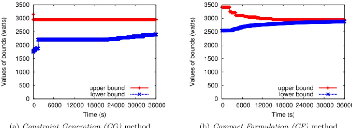
To better see the evolution of the Constraints Generation (CG) and Compact Formulation (CF) methods, we show in Fig. 8, Fig. 9 and Fig. 10, respectively the upper bound, the lower
0 500 1000 1500 2000 2500 3000 0 3000 6000 9000 12000 15000
Values of bounds (watts)
Time (s) upper bound
lower bound
(a) Constraint Generation (CG) method
0 500 1000 1500 2000 2500 3000 0 300 600 900 1200
Values of bounds (watts)
Time (s) upper bound
lower bound
(b) Compact Formulation (CF) method Figure 8: Abilene Γd= Γγ = 1%: upper bound and lower bound of CG vs. CF method
0 500 1000 1500 2000 2500 3000 3500 0 6000 12000 18000 24000 30000 36000
Values of bounds (watts)
Time (s) upper bound
lower bound
(a) Constraint Generation (CG) method
0 500 1000 1500 2000 2500 3000 3500 0 6000 12000 18000 24000 30000 36000
Values of bounds (watts)
Time (s) upper bound
lower bound
(b) Compact Formulation (CF) method Figure 9: Abilene Γd= Γγ = 10%: upper bound and lower bound of CG vs. CF method
0 10 20 30 40 50 0 3000 6000 9000 12000 15000 Optimality gap (%) Time (s) gap-CG gap-CF (a) Abilene Γd= Γγ= 1% 0 10 20 30 40 50 0 6000 12000 18000 24000 30000 36000 Optimality gap (%) Time (s) gap-CG gap-CF (b) Abilene Γd= Γγ= 10%
bound and the optimality gap obtained by CPLEX. We consider two representative cases Γγ =
Γd = 1% and Γγ = Γd = 10%. The evolution of the CF method is much better than the CG
method. As shown in Fig. 8 and Fig. 9, in CF method, both the upper and lower bounds are improving meanwhile it seems only the lower bound in CG method is improving. As shown in Fig. 9, both methods do not reach the optimality after 10 hours of computation, however, the gap of CF method is quite small (2.5%) with respect to the CG method (18.9%). However, as shown in Fig. 9a, the CG method is quite fast to obtain a good upper bound meanwhile in Fig. 9b, the CF improves the lower bound quickly. Thus, a possible idea is to get an upper bound from the CG method and a lower bound from the CF method. Then, we can use these bounds to validate the current feasible solution. Fig. 10 shows another view of the evolution: the gap between current feasible solution and optimal solution. This gap equals to zero mean the solution is the optimal one. Again, the CF method outperforms the CG method in term of improving optimality gap. Therefore, the CF method reaches the optimal point much faster than the CG method.
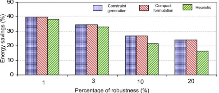
0 10 20 30 40 50 1 2 3 4 E n e rg y s a v in g s ( % ) 1 3 10 20 Constraint generation Heuristic Compact formulation Percentage of robustness (%)
Figure 11: Comparison of proposed methods on Abilene.
We show in Fig. 11 a comparison of performance between the three methods. The y-axis is the percentage of energy savings and the x-axis is the percentage of robustness over the total demand (Γ/|D|). The x-axis is cut at 20% of robustness because computed values are similar after this value. Both Γd and Γγ vary with the same value, e.g. robustness = 10% means
Γd = Γγ = 0.1×|D|. We observe that the maximum gap reported in Fig. 11 between the heuristic
and the CG (and CF) method is 7.63%, and this gap decreases for small values of Γd and Γγ.
Recall that measurements performed on real networks have shown that only a small fraction of the traffic demands deviate simultaneously from their nominal values [17]. Furthermore, the aim of robust optimization is precisely to take benefit of that fact in order to improve the design of the network, and in our case to save more energy. We have seen that our heuristic algorithm offers good performances both in terms of running time and quality of the solution in this setting. Thus in the sequel, we will use our heuristic to evaluate the Robust-GreenRE model on larger instances.
4.2.2 Energy savings vs. robustness
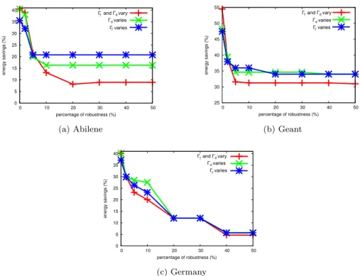
Fig. 12 shows the trade-off between energy savings and the level of robustness regarding the parameters (Γd, Γγ). We consider three test cases (1) both Γd and Γγ, (2) only Γγ and (3) only
Γd vary their values. In the Case 1, both Γd and Γγ vary with the same value of robustness.
Note that, when Γγ = Γd = 100%, all demands and compression rates are at the worst case,
therefore the Robust-GreenRE is equivalent to the deterministic GreenRE. In Case 2 (resp. Case 3), while Γγ (resp. Γd) varies, Γd (resp. Γγ) is set to 2% of the total demands. In all
0 5 10 15 20 25 30 35 40 0 10 20 30 40 50 energy savings (%) percentage of robustness (%) 1 2 3 Гd varies Г varies Г and Гd vary (a) Abilene 25 30 35 40 45 50 55 0 10 20 30 40 50 energy savings (%) percentage of robustness (%) 1 2 3 Г and Гd vary Гd varies Г varies (b) Geant 0 5 10 15 20 25 30 35 40 0 10 20 30 40 50 energy savings (%) percentage of robustness (%) 1 2 3 Г and Гd vary Гd varies Г varies (c) Germany
Figure 12: Energy savings vs. robustness for Abilene, Geant and Germany network
the three networks, the solutions do not change when Γd, Γγ ≥ |D|2 , thus the x- axis is cut
at 50%. We observe that energy savings are proportional to 1/Γ. Indeed, large values of Γ reduces the interest for robust optimization. More precisely, when Γd, Γγ ≥ 30%, energy savings
offered by the Robust-GreenRE model are almost the same as the GreenRE model, while when Γd, Γγ ≤ 20% the Robust-GreenRE model allows for significant energy savings. An explanation
of this phenomenon can be found in the distribution of the demand volumes. A small fraction of the demands dominates the others in volume. Hence, when the values of Γd, Γγcovers all of these
dominating demands, increasing Γd, Γγ does not affect the routing solution and the percentage
of energy savings remains stable. In Case 2 and Case 3, when only Γdor Γγ varies its value, the
same phenomenon is observed. It means Γdand Γγ have almost the same role in contributing to
the robustness of the network. 4.2.3 Link load
Intuitively, Robust-GreenRE would affect the utilization of links as fewer links are used to carry traffic. In this subsection, we evaluate the impact of Robust-GreenRE on link utilization. Specif-ically, we vary the level of robustness and see how the link utilization of the network is affected. We draw cumulative distribution function (CDF) of link load of Abilene, Geant and Germany networks in Fig. 13. The level of robustness is represented by percentage of traffic demands that can fluctuate in both traffic volumes and RE rates. As shown in Fig. 13, Geant and Germany networks have light traffic load. For instance, 80% of links of Geant and Germany networks are under 40% and 20% of link utilization, respectively. Traffic on Abilene network is heavier, however there is no overloaded link and 80% of links are less than 70% of utilization. In general,
0 20 40 60 80 100 0 20 40 60 80 100 Fraction of links (%) Link load (%) 5% robustness 20% robustness 100% robustness (a) Abilene 0 20 40 60 80 100 0 20 40 60 80 100 Fraction of links (%) Link load (%) 5% robustness 20% robustness 100% robustness (b) Geant 0 20 40 60 80 100 0 20 40 60 80 100 Fraction of links (%) Link load (%) 5% robustness 20% robustness 100% robustness (c) Germany
Figure 13: CDF load on Abilene, Geant and Germany networks.
traffic load is low when the level of robustness is low. For example, in Abilene network, for the case of 5% robustness, 85% of links are under 40% utilization meanwhile for the case 20% (resp. 100%) robustness, it is only 60% (resp. 40%) of links are under 40% utilization.
4.2.4 Robust-GreenRE vs. GreenRE vs. Classical EAR
0 10 20 30 40 50 1 2 3 E n e rg y sa vi n g s (% )
Abilene Geant Germany50
Network topology Г = Гd= 2% EAR Г = 5% Гd= 2% Г = 2% Гd= 5% GreenRE
Figure 14: Robust-GreenRE vs. GreenRE vs. EAR.
In Fig. 14, we compare the Robust-GreenRE model with the GreenRE and the classical EAR (no compression) models for small values of Γd and Γγ. Since the GreenRE model does not take
, γst is set to 1.0 (no compression). Furthermore, since traffic volume variations are not handle
by GreenRE and EAR models, all demands are at peak. We observe that the lowest energy savings are achieved by EAR and GreenRE models. As expected, the Robust-GreenRE model outperforms the other models and allows for 16 − 28% additional energy savings in all cases.
5
Conclusion
In this paper, we formally define and model the Robust-GreenRE problem. Taking into account the uncertainties of traffic volumes and redundancy elimination rates, the Robust-GreenRE model provides a more accurate evaluation of energy savings for backbone networks. Based on real-life traffic traces, we have shown a significant improvement of energy savings compared with other models. As future work, we shall investigate implementation issues and impacts of Robust-GreenRE model on QoS and fault tolerance.
Acknowledgment
The authors would like to thank Christelle Caillouet, Frédéric Giroire, Arie M.C.A. Koster, Joanna Moulierac and Martin Tieves for their support. This work has been partially supported by Région PACA.
References
[1] “An inefficient Truth”, http://globalactionplan.org.uk (2007).
[2] L. Chiaraviglio, M. Mellia, F. Neri, “Minimizing ISP Network Energy Cost: Formulation and Solutions”, in: IEEE/ACM Transaction on Networking, Vol. 20, 2011, pp. 463 – 476. [3] R. Bolla, F. Davoli, R. Bruschi, K. Christensen, F. Cucchietti, S. Singh, “The Potential
Impact of Green Technologies in Next-generation Wireline Networks: Is There Room for Energy Saving Optimization?”, in: IEEE Communications Magazine, Vol. 49, 2011, pp. 80 – 86.
[4] R. Tucker, J. Baliga, R. Ayre, K. Hinton, W. Sorin, “Energy consumption in IP networks”, in: Proc. ECOC Symp. Green ICT, 2008.
[5] P. Mahadevan, P. Sharma, S. Banerjee, “A Power Benchmarking Framework for Network Devices”, in: Proc. of IFIP NETWORKING, 2009.
[6] M. Gupta, S. Singh, “Greening of The Internet”, in: Proc. of ACM SIGCOMM, 2003. [7] M. Zhang, C. Yi, B. Liu, B. Zhang, “GreenTE: Power-aware Traffic Engineering”, in: Proc.
of IEEE ICNP, 2010.
[8] A. Anand, A. Gupta, A. Akella, S. Seshan, S. Shenker, “Packet Caches on Routers: the Implications of Universal Redundant Traffic Elimination”, in: Proc. of ACM SIGCOMM, 2008.
[9] A. Anand, C. Muthukrishnan, A. Akella, R. Ramjee, “Redundancy in Network Traffic: Findings and Implications”, in: Proc. of ACM SIGMETRICS, 2009.
[10] Y. Song, K. Guo, L. Gao, “Redundancy-aware Routing with Limited Resources”, in: Proc. of IEEE ICCCN, 2010.
[11] E. Zohar, I. Cidon, “The Power of Prediction: Cloud Bandwidth and Cost Reduction”, in: Proc. of ACM SIGCOMM, 2011.
[12] P. H. Srebrny, T. Plagemann, V. Goebel, A. Mauthe, “No More Deja Vu - Eliminating Redundancy With CacheCast: Feasibility and Performance Gains”, in: IEEE/ACM Trans-action on Networking, Vol. PP, 2013.
[13] F. Giroire, J. Moulierac, T. K. Phan, F. Roudaut, “Minimization of Network Power Con-sumption with Redundancy Elimination”, in: Proc. of IFIP NETWORKING, LNCS 7289, 2012, pp. 247 – 258.
[14] D. Bertsimas, M. Sim, “Robust Discrete Optimization and Network Flows”, in: Math. Prog., Vol. 98, 2003, pp. 49 – 71.
[15] D. Bertsimas, M. Sim, “The Price of Robustness”, in: Operations Research, Vol. 52, 2004, pp. 35 – 53.
[16] A. M. C. A. Koster, M. Kutschka, C. Raack, “On the Robustness of Optimal Network Designs”, in: Proc. of IEEE ICC, 2011.
[17] A. M. C. A. Koster, M. Kutschka, C. Raack, “Robust Network Design: Formulation, Valid Inequalities, and Computations”, in: Networks, Vol. 61, 2013, pp. 128 – 149.
[18] D. Coudert, A. Koster, T. K. Phan, M. Tieves, “Robust Redundancy Elimination for Energy-aware Routing”, in: Proc. of IEEE GreenCom, 2013.
[19] G. Classen, A. Koster, A. Schmeink, “A Robust Optimisation Model and Cutting Planes for The Planning of Energy-efficient Wireless Networks”, in: Journal of Computers and Operations Research, Vol. 40, 2013, pp. 80 – 90.
[20] D. Bertsimas, D. B. Brown, C. Caramanis, “Theory and Applications of Robust Optimiza-tion”, in: Journal SIAM Review, Vol. 53, 2011, pp. 464–501.
[21] F. Giroire, D. Mazauric, J. Moulierac, B. Onfroy, “Minimizing Routing Energy Consump-tion: from Theoretical to Practical Results”, in: Proc. of IEEE/ACM GreenCom, 2010. [22] N. T. Spring, D. Wetherall, “A Protocol-Independent Technique for Eliminating Redundant
Network Traffic”, in: Proc. of ACM SIGCOMM, 2000, pp. 87 – 95.
[23] A. Anand, V. Sekar, A. Akella, “SmartRE: an Architecture for Coordinated Network-wide Redundancy Elimination”, in: Proc. of ACM SIGCOMM, 2009.
[24] “BlueCoat: WAN Optimization”, http://www.bluecoat.com/.
[25] T. J. Grevers, J. Christner, “Application Acceleration and WAN Optimization Fundamen-tals”, in: Cisco Press, 2007.
[26] Http://www.riverbed.com/us/solutions/wan_optimization/.
[27] A. Ben-Tal, L. El Ghaoui, A. Nemirovski, “Robust Optimization”, Princeton Series in Ap-plied Mathematics, 2009.
[28] A. Ben-Tal, A. Nemirovski, “Robust Optimization - Methodology and Application”, in: Math. Prog., Vol. 92, 2002, pp. 453 – 480.
[29] A. Altin, E. Amaldi, P. Belotti, M. C. Pinar, “Provisioning Virtual Private Networks under Traffic Uncertainty”, in: Networks, Vol. 49, 2007, pp. 100 – 115.
[30] S. Duhovniko, A. M. C. A. Koster, M. Kutschka, F. Rambach, D. Schupke, “Γ-Robust Network Design for Mixed-Line-Rate-Planning of Optical Networks”, in: Proc. Optical Fiber Communication - National Fiber Optic Engineers Conference (OFC/NFOEC), 2013. [31] A. Koster, T. K. Phan, M. Tieves, “Extended Cutset Inequalities for the Network Power
Consumption Problem”, in: Electronic Notes in Discrete Mathematics, Vol. 41, 2013, pp. 69 – 76.
[32] IBM ILOG, CPLEX Optimization Studio 12.4 (2012).
[33] S. Orlowski, R. Wessäly, M. Pióro, A. Tomaszewski,
SNDlib 1.0 - survivable network design library, Networks 55 (3) (2010) 276–286. URL http://sndlib.zib.de

![Figure 4: Traffic demands in Abilene network [17]](https://thumb-eu.123doks.com/thumbv2/123doknet/13108557.386552/12.892.241.599.184.364/figure-traffic-demands-in-abilene-network.webp)