HAL Id: hal-02114528
https://hal-normandie-univ.archives-ouvertes.fr/hal-02114528
Submitted on 29 Apr 2019
HAL is a multi-disciplinary open access
archive for the deposit and dissemination of
sci-entific research documents, whether they are
pub-lished or not. The documents may come from
teaching and research institutions in France or
L’archive ouverte pluridisciplinaire HAL, est
destinée au dépôt et à la diffusion de documents
scientifiques de niveau recherche, publiés ou non,
émanant des établissements d’enseignement et de
recherche français ou étrangers, des laboratoires
Specularity removal: a global energy minimization
approach based on polarization imaging
Fan Wang, Samia Ainouz, Caroline Petitjean, Abdelaziz Bensrhair
To cite this version:
Fan Wang, Samia Ainouz, Caroline Petitjean, Abdelaziz Bensrhair. Specularity removal: a global
energy minimization approach based on polarization imaging. Computer Vision and Image
Under-standing, Elsevier, 2017. �hal-02114528�
Specularity removal: a global energy minimization
approach based on polarization imaging
Fan Wanga,b,⇤, Samia Ainouzb, Caroline Petitjeanb, Abdelaziz Bensrhairb aResearch Institute of Intelligent Control & Image Engineering, Xidian University, 710071,
Xi’an, China
bLITIS laboratory, INSA de Rouen, 76801, Saint-Etienne du Rouvray, France
Abstract
Concentration of light energy in images causes strong highlights (specular re-flection), and challenges the robustness of a large variety of vision algorithms, such as feature extraction and object detection. Many algorithms indeed assume perfect di↵use surfaces and ignore the specular reflections; specularity removal may thus be a preprocessing step to improve the accuracy of such algorithms. Regarding specularity removal, traditional color-based methods generate severe color distortions and local patch-based algorithms do not integrate long range information, which may result in artifacts. In this paper, we present a new im-age specularity removal method which is based on polarization imaging through global energy minimization. Polarization images provide complementary infor-mation and reduce color distortions. By minimizing a global energy function, our algorithm properly takes into account the long range cue and produces ac-curate and stable results. Compared to other polarization-based methods of the literature, our method obtains encouraging results, both in terms of accuracy and robustness.
Keywords: specularity removal, polarization, di↵use, separation, energy minimization
⇤corresponding author
1. Introduction
Based on the dichromatic reflection model [1], each brightness value in an image is viewed as the sum of two components, the di↵use and the specular parts. Most opaque surfaces have a combination of specular and di↵use elements due to surface structure. The di↵use element is viewable from all directions
5
while the specular part behaves based on Snells law [2], so is only visible when viewed from the correct orientation. The specular reflection appears to be a compact lobe on the object surface around the specular direction, even for rough surfaces [3]. Whereas the di↵use component represents the actual appearance of an object surface, specularity reflection is an unwanted artifact that can
10
hamper high-level processing tasks such as visual recognition, tracking, stereo reconstruction, objects re-illumination [4, 5]. Specularity removal, a challenging topic in computer vision, is thus a decisive preprocessing for many applications [6].
1.1. Related works
15
The light reflection always carries important information of a scene, so that the separation of the reflection gives a way to better analyze the scene. Nayar et al. [7] separates the reflection using structured light, which conveys useful properties of the object material as well as the media of the scene. O’Toole et al. [8] also use structured light in reflection separation to recover the 3D
20
shape of the object. While the above methods have shown good performance in their applications, they analyze the scene through the direct and global re-flection components, whereas we analyze it through the specular and di↵use reflections. Direct components contain both specular and di↵use reflections, while global components arise from interreflections as well as from volumetric
25
and subsurface scattering. The direct/global separation handles complex re-flections, which may result in useful material related information ; however it requires strict controllable light source, which limits this usability of this sepa-ration. On the other hand the specular/di↵use component analysis deals with
natural light source, which makes it more valuable. The separation of
specu-30
lar/di↵use components is thus regarded as pre-processing step, since specular reflection might be problematic in several computer vision tasks, such as stereo matching, image segmentation or object detection.
There are also works that aim at separating the di↵use and specular compo-nents under polarized light source. For instance, in [9] a robust di↵use/specular
35
reflection separation method is proposed, but is designed to only work for scene under controllable light source. In this work, we take a di↵erent approach leading to a generalization of the applicability: we deal with scenes under un-controllable light source, in order to imitate outdoor illumination conditions.
Traditional methods separate the di↵use and specular components using
40
color-only images, based on the idea to find a variable which is independent from the specular component. By estimating this variable for each given pixel, the di↵use component may be computed. As a seminal work in color-based methods, Tan et al. [10] inspects the specular component via chromaticity, which is proved to be independent from the specular component. An additional
45
hue-based segmentation method is required for the multi-colored surfaces. Yang et al. [11] extend this work by detecting di↵use pixels in the HSI space, which also requires hue-based segmentation. The color covariance is defined as a con-stant variable to recover the di↵use component. Kim et al. [12] use the dark channel prior as a pseudo-solution and refine the result through the Maximum
50
A Posteriori (MAP) estimation of the di↵use component. The dark channel prior, however, only works for highly colored surfaces. To avoid extra segmen-tation, Tan and Ikeuchi [13] propose another di↵use pixel pick-up method via computing the logarithmic di↵erential between up to four neighboring pixels. The common limitation of the above presented color-based methods is their high
55
color distortion on the recovered di↵use component [13, 3, 11]. The main reason is that these methods assume that the specular color is constant throughout the image.
To better recover the di↵use component, other methods proposed to accom-plish the separation using polarization images [14], since specular and di↵use
components hold di↵erent degrees of polarization (DOP). The DOP represents the ratio of the light being polarized. When a beam of unpolarized light is re-flected, the DOP of specular reflection is larger than that of the di↵use reflection for most angles of incidence, meaning that the specular reflection is generally much more polarized than the di↵use reflection [15]. When rotating the
polar-65
izer, the change of the intensity is only related to the specular part, so that the intensity change refers directly to the specular color.
With these constraints, polarization based methods produce more accurate results with less color distortions. The pioneering work of Nayar et al. [3] constrains the di↵use color on a line in RGB space. The neighboring
di↵use-70
only pixels are used to estimate the di↵use component, providing state-of-the-art polarization-based specularity removal results. However, specular pixels are detected by simple tresholding of the DOP. The DOP changes not only with di↵erent specular portions, but also with di↵erent incident angles and di↵erent indices of refraction. The computation of the DOP involves more than three
75
images, making it largely contaminated by camera noise. This makes Nayar’s method prone to error since its computation highly relies on the DOP.
The methods presented above are local and based on the dichromatic re-flection model [1]. These methods assume that the intensity of a pixel is a linear combination of its di↵use and specular components. On the other hand,
80
a global-based method presented in [16] simplifies this model into the image level, under the conditions that the light source is far away from the object and that the incident angle does not change. In other words, the acquired image is linearly combined by a specular image and a di↵use image with respect to a constant parameter. This parameter is reversed using the Independent
Com-85
ponent Analysis (ICA) [17]. However, these ideal conditions discussed in [16] rarely conform to reality, thus only a part of the specular reflection component is removed.
With respect to the literature, we make the following observations: (i) color-based methods produce heavy color distortions; (ii) local patch-color-based methods
90
consid-eration of long range cues. Based on these observations, we proposed in this article a global method using the polarization setup and a local approximate solution as detailed in the next subsection.
1.2. Contribution
95
Our approach builds upon Umeyama’s method [16] and share conceptual similarities. However, we propose a threefold contribution : (i) As in [16] we as-sume that the acquired image is the linear combination of a di↵use and specular reflection images. However, we depart from the use of a fixed weighting coeffi-cient and instead investigate the benefit of using a spatially varying coefficoeffi-cient,
100
which generalizes the model proposed in [16] to better conform to the reality. The use of the spatially varying parameter additionally enables the algorithm to work with scenes under (non-overlapping) multi-sources of illumination. (ii) Based on these assumptions, a global energy function is constructed to leverage long range information, that patch based method cannot handle, by
construc-105
tion. In patch based methods, the solution for one pixel is influenced only by the local neighborhood. In a graph based approach, pixels are connected through the graph construction, and their interdependency is accounted thanks to the smoothness term; additionally, the graph energy is minimized globally. The expectation is that by optimizing the problem globally, results will be more
110
accurate and robust than with local patch-based methods. The optimum solu-tion is found by applying the graph cuts algorithm [18]. (iii) Apart from the independence assumption, a first approximate solution is computed as a sup-plementary constraint. We propose to compute a more reliable approximate solution by combining the specular detection method in [13] and the specularity
115
reduction in [3]. Lastly, in the experimental part, a histogram-based criterion is proposed to quantitatively evaluate the results. The proposed method is compared with two well-known separation algorithms : Nayar’s polarization setup [3] and Umeyama’s method [16]. This paper extends upon our previous preliminary work [19] in the following aspects. In the current paper, we fully
120
solution. The computation of the data term is accurately described, as well as the smoothness term, and the justification as to why the solution is ensured to be stable. This paper contains some additional illustration to demonstrate more clearly the improvement of the proposed global method. Supplementary
125
experiments are also reported, including the study of the algorithm robustness in the presence of noise.
1.3. Overview
In the remainder of the paper, we first present our polarization system in Section 2. The problem formulation is defined in Section 3. In section 4, we
130
describe the proposed global energy function, and explain each term in detail. In Section 5, we describe the implementation of the method with a discussion about the results. Finally, we o↵er some perspectives to this work in Section 6.
2. Polarization system
The light reflection from an object is a combination of di↵use and specular
135
components, in which the specular component is generally partially linearly po-larized. It is fully described by three parameters [20]: light magnitude I, degree of polarization ⇢, angle of polarization '. In order to measure the polarization parameters, a polarizer rotated by an angle ↵ is installed in front of the camera as shown in Fig. 1 (a). Several images Ip(↵i) are acquired by rotating the
polar-140
izer to di↵erent positions ↵i. The intensity Ip(↵i) of each pixel is linked to the
polarizer angle ↵i and the polarization parameters by the following equation:
Ip(↵i) =
I
2[⇢cos(2↵i 2') + 1] (1)
Since there are three unknown parameters (I, ⇢ and ') to be determined in Equation (1), at least three images need to be acquired with di↵erent ↵i. Fig.
1 (b) shows the variation curve of I(↵i), where for each pixel, Imax and Imin
145
refer to the maximum and minimum intensity, respectively.
Regarding the number of images to be acquired, di↵erent configurations are possible, such as 36 images in [21]. The more images are acquired, the
Intensity Imax Imin Polarizer CCD Camera Light (a) (b)
Figure 1: (a) Polarization imaging system; (b) Variation of intensity by rotating the polarizer angle ↵.
more stable the results will be. However, in this paper, we chose to use three images since current hardware capture no more than three polarization images
150
simultaneously [22], and since we aim at solving this problem for potentially real-time applications.
Once all three parameters have been estimated, Imaxand Imincan be
com-puted thanks to:
I = Imax+ Imin, ⇢ = Imax Imin Imax+ Imin (2) 3. Problem formulation 155
From the dichromatic reflectance model [23], a beam of light is a linear combination of the di↵use and specular components. Umeyama et al. [16] have simplified this model to the image level by assuming that the acquired image I is the sum of a di↵use image Id and a specular image Is, where the Is is a raw
specular image ˚Iscombined with a fixed weighting coefficient p as shown in Fig.
160
2 (a). The image I is thus related to its components according to: 8 > < > : I(x) = Id(x) + Is(x) Is(x) = p˚Is(x) (3)
= × +
fix coefficient spatially varying mixing coefficient(a)
(b)
p(x)
= p × +
I
I
s
I
d
raw specular componentI
os
Figure 2: Modeling an image I as a linear combination of a di↵use component Idand a raw
specular component Is, with (a) a fixed coefficient as in Umeyama et al. [16], it can be seen
that the specular component is not fully removed from Id; (b) a spatially varying coefficient
as assumed in our approach, which more e↵ectively removes the specular reflection.
The raw specular image ˚Is is defined as:
˚Is= Imax Imin (4)
where Imax and Imin are the maximum and minimum intensity described in
Equation (2). The goal is to estimate p, as then the corresponding di↵use Id(x)
and specular components Is(x) can be computed using Equation (5). The di↵use
165
and specular reflection images being assumed probabilistically independent, the optimum p can be found by minimizing the Mutual Information (MI) [24, 16] between Id and Is to ensure their maximum independence.
This method globally models the di↵use and specular separation problem, however it su↵ers from some limitations. First, in real applications, the
assump-170
tion that the incident angle on each pixel remains constant is not always valid. Hence, setting a single value for the weighting coefficient over the whole image is inconsistent. As a consequence, the computation of MI, which is
computa-tionally costly, becomes unfeasible or at least unrealistic1, since the sum of MI
needs to be minimized at each local patch.
175
We propose to tackle these limitations through the following improvements: (i) The mixing coefficient is assumed to be spatially varying as shown in Fig. 2(b). As one can see, the specular reflection is more e↵ectively removed from the computed di↵use component in Fig. 2(b) than in Fig. 2(a); (ii) As in [16] We assume that Id and Is are probabilistically independent. The goal is
180
to minimize their similarity. Since only maximizing the independence is not enough to produce the best solution, we introduce a first approximate solution as a constraint to ensure the reliability of the final solution; (iii) Instead of MI, we propose to compute another more efficient similarity measurement which produces competitive results.
185
4. Global energy function
As global methods can better integrate the long range cue via the global smoothness assumption, they can produce more accurate and robust result than local patch-based methods. For this purpose, we propose a global energy func-tion, which is composed of a data term and a smoothness term.
190
As mentioned above, in this paper we assume that the mixing coefficient is spatially varying. Equation (3) is transformed into:
8 > < > : I(x) = Id(x) + Is(x) Is(x) = p(x)˚Is(x) (5)
where the p(x) is the local weighting coefficient.
From Umeyama et al. [16], the specular component p(x)˚Is(x) is decided by
the surface geometry and the angle of incidence of the light which is generally
195
locally smooth. As ˚Is(x) represents the unit color vector of pixel x, we make
a smooth assumption on the term p(x), which enforces the continuity of the
1on a laptop running with a 2.6 GHz processor and 8GB RAM.for about 25 minutes for a
specular component. To consider the sharp change that might originate from the di↵erent structures of the scene, we have included a color discontinuity detection method in Section 4.2. Our objective is to find an optimum p(x) for
200
each pixel x.
Let (p(x)) denote the data term and (p(x), p(y)) the smoothness term of the global energy function. The optimum p(x) can be found by solving the following constraint optimization problem:
argmin p(x) X x (p(x)) + 1 X x X y2N (x) (p(x), p(y))] s.t. 0 p ˜p (6)
where y 2 N (x), N (x) refers to the 4-connected neighborhood of x, 1 is a
205
hyper-parameter which balances the data and the smoothness terms. While solving the minimization problem, a large p value may result in a negative intensity of Id(from Equation (5)). For this reason, pixel-wise dependent scalar
˜
p is applied on p as an upper bound, so that Id is always kept positive.
4.1. Minimization algorithm: graph cuts
210
This energy function in Equation (6) is solved by using the graph-cut algo-rithm. The image is considered as a graph: each pixel is represented by a node, and the edge weights between nodes are related to the similarity between the nodes (smoothness term in Eq (6)). Each node is also linked so special nodes which express the constraint given by the problem knowledge, i.e. the data term
215
in Eq (6). A graph cut is a partition of the graph (i.e. the image). Each pos-sible partition has a cost, which can be expressed as the sum of the weights of the edges cut when partitioning. The optimum segmentation is the lowest-cost cut in the graph, and it can be efficiently solved using the ↵-expansion [18], an algorithm well-known for its e↵ectiveness in solving large global optimization
220
4.2. Data term
The data term (p(x)) contains two parts: a patch-based dissimilarity (in-dependence) measurement CDC(p(x)), and a pixel-wise constraint D(p(x)):
(p(x)) = 2CDC(p(x)) + D(p(x)) (7)
where 2 is a weighting hyper-parameter. The term CDC(p(x)) is used to
max-225
imize the independence between the di↵use and the specular images. However, using this term only tends to over-smooth the solution, leading us to introduce an additional constraint in this data term, denoted D(p(x)). This constraint is based on an initial approximate solution and enforces the similarity between the final solution and this initial result. Using an initial solution has several
230
advantages: first, it ensures the reliability of the result. In addition, the first solution used as the initialization to the optimization process also improves the time efficiency. By minimizing (p(x)), the optimum p(x) is found through the trade-o↵ between maximizing CDC(p(x)) and minimizing D(p(x)).
4.2.1. Dissimilarity measurement
235
Dissimilarity between di↵use and specular images is usually measured through mutual information [16]. Since using mutual information for a patch centered at each pixel is highly time consuming, we take advantage of another criterion, which from our experiments, yields similar results as compared to mutual in-formation and is less time consuming. This criterion, called DIF F census [26]
240
has been shown to be an efficient criterion to optimize the disparity map. It is known to be resistant to noises and color distortions.
Let us now define the DIF F census cost function. Given a pixel location x and an arbitrary p(x) (0 p(x) ˜p(x)), the independence between the di↵use component Id(x) and its corresponding specular component Is(x) is measured
245 with: CDC(p(x)) = DIF F census(Id(x), Is(x)) = g(Ccensus( ¯Id(x), ¯Is(x)), census) + g(CDIF F( ¯Id(x), ¯Is(x)), DIF F) (8)
where g(C, ) = 1 exp( C), and ¯Id(x) and ¯Is(x) are n⇥ m patches centered
at x with arbitrary size (n = m = 5 in our experiments). DIF F and census
are hyperparameters balancing the two parts, set to default values DIF F = 55
and census = 95 as suggested in [26]. More specifically, in Equation (8), we
250 have: 8 > < > : Ccensus( ¯Id(x), ¯Is(x)) = H(CT ( ¯Id(x)), CT ( ¯Is(x))) CDIF F( ¯Id(x), ¯Is(x)) = |DIF F ( ¯ Id(x)) DIF F ( ¯Is(x))| n⇥ m (9)
where CT (·) refers to the Census Transform, and H(·) is the Hamming distance. For more information about CT and Hamming distance, please refer to [27]. DIF F (·) is computed as:
8 > < > : DIF F ( ¯Id(x)) =Py2 ¯Id(x)|Id(x) Id(y)| DIF F ( ¯Is(x)) =Py2 ¯Is(x)|Is(x) Is(y)| (10)
The DIF F census function represents a trade-o↵ between the classical CT and
255
the Sum of Absolute Di↵erence which are balanced via hyperparameters DIF F
and census. Results are improved compared to using these criteria alone [26].
4.2.2. Constraint term
The independence assumption alone does not provide a good separation result. In order to guide the separation process, we introduce a constraint on
260
the final solution p(x) to enforce its similarity to a first approximate solution pinit(x). The constraint term is given by measuring:
D(p(x)) =|p(x) pinit(x)| (11)
The first approximate solution pinit(x) is found by combining the logarithm
di↵erential specular detection method proposed by [13] and the specular-to-di↵use mechanism in [3]. The computation of pinit(x) is detailed in Section
265
4.2.3. Stability of the solution
The aim of the data term is to find p(x) that numerically minimizes (p(x)). The problem is to find a trade-o↵ between maximizing CDC and minimizing
D(p(x)) so that the final solution does not go randomly far from an approximate
270
solution pinit. The minimum of this functional cannot degenerate to infinity
because our space is of finite dimension (pixels) and the functional (p(x)) is continuous and bounded from below. Let us demonstrate these points. By construction, the research space of the solution p(x) is in the domain [0, ˜p(x)] (0 p(x) ˜p(x)) where ˜p(x) 2 [0, 255] is an upper bound so that the di↵use
275
image Idis always positive. The minimum of the functional (p(x)) is searched
within this domain.
Regarding the CDC term, from the Equation (8), it is a combination of two
functions g, where g(x) = 1 exp( x) and is bounded by 1. Thus
CDC(p(x)) = g(Ccensus, census) + g(CDif f, Dif f) < 2 (12)
Regarding the D(p(x)) term, it is the absolute value of the di↵erence between
280
p(x) and the first approximate solution pinit. D(p(x)) is thus positive and finite
also because 0 p(x) ˜p(x).
Consequently, (p(x)) has a lower bound, ensuring the stability of the solu-tion:
(p(x)) = 2CDC(p(x)) + D(p(x)) > 2 2 (13)
4.3. Smoothness term
285
The smoothness term is classically computed among the 4-connected neigh-borhoodN (x) of the pixel x. To better take into account the original texture of the image, we implement a color discontinuity detection based on thresholding RGB values, as suggested in [13]. Let T hR and T hG be small threshold values (one should adjust this value according to the input images, here default values
290
T hR = T hG = 0.005 as in [13] are used in this paper), and indices r and g be the red and green channels in the RGB space. A color discontinuity on the pixel
x is defined as follows: ( r(x) > T hR and g(x) > T hG) 8 > < > :
true: color discontinuity false: no color discontinuity
(14) where 8 > < > : r(x) = r(x) r(x 1) g(x) = g(x) g(x 1) (15) and 295 8 > > < > > : r= Ir Ir+ Ig+ Ib g= Ig Ir+ Ig+ Ib (16)
Chromaticity changes are computed between neighboring pixels on both red and green channels (the blue channel is not included since r+ g+ b= 1). This
method detects the color discontinuity, which helps to maintain the original texture of the object, as well as to prevent the smoothness term from running over the object boundary (where the sharp change of the object shape appears).
300
The smoothness term is defined as: (p(x), p(y)) =
8 < :
0, if x is located on a color discontinuity p
p(x)2 p(y)2 otherwise (17)
4.4. First approximate solution
The first approximate solution pinit(x) provides an additional constraint to
the data term to improve the accuracy of the model, as well as a sub-optimal initial solution to improve the efficiency of the subsequent optimal process.
305
To locally obtain an approximate solution, we propose two steps: spec-ular region detection and specspec-ularity reduction. For specularity detection, polarization-based methods usually apply a simple thresholding on the DOP as in [3], which is unreliable because of noise. Also the threshold largely varies from scene to scene. Thus we will rely upon Tan’s approach [13]. For
specu-310
RGB, there is no color constraint whereas there is one for polarization images. Tan’s method does not fully make use of the richness of polarization images. For this reason, we propose Nayar’s approach [3]. In the following, we describe each step of specularity detection and reduction and how we propose to combine
315
them sequentially.
4.4.1. Specularity detection
For RGB images, Tan notices in [13] that making the pixel saturation con-stant with regard to the maximum chromaticity while retaining their hue, allows to successfully remove highlights. The chromaticity is defined as the normalized
320
RGB:
⇤(x) = I(x)
Ir(x) + Ig(x) + Ib(x)
(18) where ⇤ ={⇤r, ⇤g, ⇤b}. The maximum chromaticity is defined as :
˜
⇤(x) = max(Ir(x), Ig(x), Ib(x)) Ir(x) + Ig(x) + Ib(x)
(19) For the whole image, the I(x) is shifted so that the maximum chromaticity ˜
⇤(x) is turned to an arbitrary constant value (we set ˜⇤(x) = 0.5 as suggested by [13]), yielding a new image I0, where highlights are removed. However this
325
method yields color distortions in I0 and is limited to weak specular highlights. Thus, a logarithm di↵erential step is added. Let y be a neighboring pixel of x, the logarithm di↵erential (x, y) is computed as:
(x, y) = logI(x) I(y) log
I0(x)
I0(y) (20)
Tan shows indeed that if two neighboring pixels are both di↵use pixels, their intensity logarithm di↵erential is zero, meaning that their log ratio still keeps
330
the same between I and I0. Otherwise, if they are not on the color discontinuity, they should be both specular pixels. The ambiguity between specular and color discontinuity is suppressed via the color discontinuity detection described in Equation (14).
I
dI
sB
R
G
LI
maxI
minD
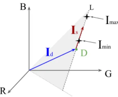
Figure 3: Di↵use Idand specular Iscomponents in RGB space
4.4.2. Specularity reduction
335
The aim of this step is to find the specular part and the di↵use part of the so-called specular pixels, obtained from the preceding step. The main idea, based on Nayar et al. [3], is to assume that neighboring pixels have the same di↵use part. Thus the (known) di↵use part of the di↵use-only pixels (computed in Section 4.3.1) will be used to assess the di↵usion part of the specular pixels.
340
Let us recall that a specular pixel intensity is the sum of a di↵use component (Id) and a specular component (Is), and that it lies on a line defined by Imin
and Imax. This line is the color constrain that can be obtained only through
polarization. The line L is determined using the Imax and Imin found through
Equation (1). Since only the specular component Isis polarized [14], by rotating
345
the polarizer, I(x) varies along the line L.
The process starts with specular pixels which are located at the edges of the specular region; for all of these pixels xi belonging to the borders, its di↵use
parts is computed as the mean of the di↵use part of their di↵use-only neighbors yj.
350
Note that not all neighboring pixels are used, only those which are close enough to the plane defined by the origin of the RGB space and L in Fig. 3, by checking if the angle between I(yj) and this gray plane is inferior to a threshold.
The process is repeated iteratively. During the process, the components of di↵use only pixels are used, or the di↵use component of pixels for which has
355
(a)
(b)
(c)
Figure 4: (a) Original image; (b) First approximate solution Pinit; (c) Final solution P by
the proposed method
the process yields the pinit(x) map, the first approximate solution, equal to 0
for di↵use-only pixels and to a non zero value for specular pixels.
5. Experimentation 5.1. Implementation and data
360
In the experiments, we compare the proposed approach to two well-known methods in the literature: Nayar’s method [3] which provides the state-of-the-art local specular and di↵use separation using polarization; Umeyama’s method which is a global polarization-based algorithm. The algorithm is implemented on Matlab 2012a and a C++ platform, and the energy function is solved through
365
graph cuts with 4-connected neighbors using the gco v3.0 library [18, 28, 29]. The problem of optimizing p(x) is formulated as a global labeling problem, with labels ranging from 0 to 255. Regarding hyperparameters, it is worth to note that the specularity removal results are stable for 1 in the range [3.5, 7] and
for 2in the range [1.3, 1.7], regardless of the processed image. In the following
370
experiments, hyperparameters are 1 = 5 (in Equation (6)) and 2 = 1.5 (in
Equation (7)).
As far as we know, there is no public polarization-based benchmark. The proposed approach is evaluated on six images acquired with a polarization
de-vice composed by a polarizer2 and a CCD camera3. In order to foster fair
375
bench-marking of specular removal methods on common data, we have made our images available4.
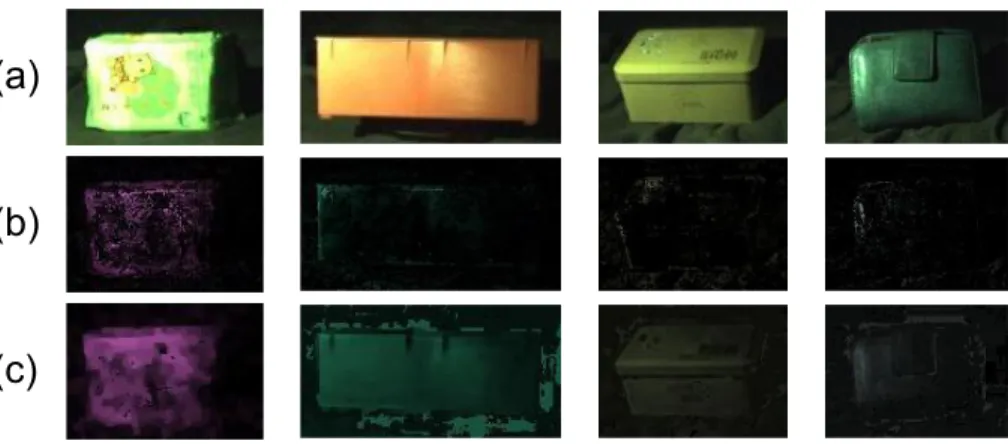
5.2. Visual evaluation
In order to visually assess the specular part, we show four groups of images (Fig. 4 (a)) with their first approximate solution Pinit (Fig. 4 (b)) and their
380
final solution P (Fig. 4 (c)) given by our global method.
Let us now visually assess the specularity removal on the di↵use component. We show the results of six groups of images (Fig. 5 (a)) with four methods, Umeyama’s method [16] (Fig. 5 (b)), Nayar’s method [3] (Fig. 5 (c)), our first approximate solution (Fig. 5 (d)) and the proposed final solution (Fig. 5 (e)).
385
Umeyama’s method removes only a small part of the specular component, with a reduction on the contrast. The reason is that the assumption of uniform incident angle made by Umeyama does not hold on real images. It also proves that the independency assumption alone is not able to yield a good result. The first ap-proximate solution that we computed shows obvious improvement. Results are
390
similar but slightly better than Nayar’s, where we can see that the specularity is only partially removed. Interesting to note is that the significant gain originates from the first approximation. Since it is easy to compute, this approximation may show promise for real-time operation. In order to further increase accuracy, the global method leverages the independency assumption and the constraint
395
given by the first approximate solution, so as to handle the remaining noise, and detect and remove more completely the specular component.
(b) (c) (d) (e) (a) Group 1 Group 2 Group 3 Group 4 Group 5 Group 6 0.0397 0.0370 0.0339 0.0330 0.0184 0.0261 0.0251 0.018 0.0114 0.0122 0.0113 0.0078 0.0274 0.0193 0.0189 0.0173 0.0100 0.0065 0.0053 0.0049 0.0419 0.0322 0.0268 0.0281
Figure 5: (a) Original image; (b) Results of Umeyama’s method; (c) Results of Nayar’s method; (d) First approximate solutions; (e) Results of the proposed method. The SD is given for each result image. Figure best viewed in color.
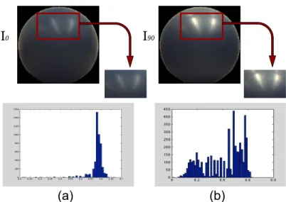
I
0I
90(a)
(b)
Figure 6: Histogram of hue values with (a) I0, weak specular reflection; (b) I90, strong specular
reflection
5.3. Quantitative evaluation
In the literature, only visual comparison of results from di↵erent methods is usually given, without any quantitative evaluation [13, 3, 30]. The reason is
400
that, first, a ground truth is not always accessible; Second, the ground truth is usually acquired under an extreme dark illumination and thus not usable for error computation.
However we propose to evaluate the specularity removal results using the Standard Deviation (SD) of the histogram distribution. Let us illustrate this
405
criterion on an object with uniform color (hue) in Fig. 6. I0is acquired with a
polarizer positioned at 0oand I
90at 90o. These images are analyzed in the HSV
space, since the chromaticity is straightforwardly presented as hue in this color space. The histogram of hue values with weak specular reflections (Fig. 6 (a))
2http://www.edmundoptics.fr/optomechanics/optical-mounts/
polarizer-prism-mounts/rotary-optic-mount/1978/
3http://www.theimagingsource.com/en_US/products/cameras/gige-cmos-ccd-color/
dfk33gv024/
is more concentrated than the one with strong specular reflections (Fig. 6 (b)).
410
Standard deviation of hue values can thus be used to quantize the quality of specularity removal: the smaller the SD is, the better the specular component is removed. Note that this criterion is applicable only for images where the specular reflection does not cover the majority of the image, and where the texture of the original image is relatively simple.
415
The SD is computed for each resulting image in Fig. 5. It can be noted that our proposed method also produce the best results as already observed qualitatively, followed by the first approximate solution and Nayar’s method [3]. Umeyama’s method [16] always produces the largest SD, except on group 5, which is hampered by a large whitening e↵ect leading to a relatively small
420
SD value. However, when taking into account both the visual and quantitative evaluations, we can conclude that our method still produces the best specularity removal results on this set of images.
However room for improvement is left regarding the computation time. In-deed, for a 240⇥ 320 pixel image, the execution time of the specularity removal
425
takes approximately 1.5 second for Umeyama’s method, 7 seconds for Nayar’s method, and 10 seconds for the proposed method, including computing the first approximate solution, data term and the optimization process, all measured on a laptop running with a 2.6 GHz processor and 8GB RAM.
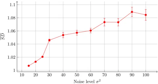
5.4. Robustness analysis
430
Local-based methods are usually based on the DOP. Since the DOP is com-puted from at least three images, it is largely contaminated by noise. Local-based methods are hence prone to su↵er from noise. This motivates us to analyze the performance of our method with respect to di↵erent noise levels.
White Gaussian noise with zero mean and varying values of is added to I0,
435
I45and I90. The SD of each group of images are computed correspondingly. Let
SD0be the SD of the result without noise, SD is normalized as SD = SD/SD0.
It is straightforward that when SD is near to 1, it means that SD is nearly equal to SD0, and the result is not largely influenced by noise. The mean (red point)
10 20 30 40 50 60 70 80 90 100 1 1.02 1.04 1.06 1.08 1.1 Noise level 2 SD
Figure 7: Quality of image with removed specularity w.r.t. added Gaussian noise: Mean SD over the 6 images vs noise level 2. The error bar refers to the variance of SD over the 6
images.
and the variance (error bar) of SD over the groups of Fig. 5 are computed and
440
shown in Fig. 7.
For 2< 20, little variation on SD can be noticed. It can be seen that even
by adding noise with 2 = 25, which is considerable, SD still remains close to
1, and the change of SD is small, inferior to 5%. That is to say, our method remains stable against noise with 2 25. Note that noise with 2> 25 rarely
445
appears in real application thanks to improved camera quality. This experiment gives us some insight about the encouraging behavior of our method regarding robustness.
6. Discussion and future work
In this paper, we proposed a polarization-based global energy minimization
450
approach to remove the specular component from images. This method is based on an independence assumption, with constraints given by a first approximate solution. Polarization information is used as a color constraint which largely reduces the color distortion produced by traditional color-based methods. The
robustness analysis also shows that the proposed method is stable for camera
455
noise, which is quite problematic for classical local methods.
Regarding the data term of the global energy function, as a tradeo↵ between maximizing (p(x)) while minimizing D(p(s)) is to be found, it has been simply and intuitively defined as the sum of a positive term and a negative term. Alternatives include maximizing (p(x))/D(p(s)) or the log di↵erence. Future
460
study may focus on a way to improve the design of the data term. To further improve the e↵ectiveness of the smoothness term, we may want to consider to combine the (·) (Equation (6)) with the local intensity or the gradient of the intensity, as future work. In this way, the object boundary may be better preserved.
465
The chromaticity information is essential in finding the first approximate solution, since the latter one is largely dependent on the variation of the chro-maticity in terms of the specular component. If the specular component and the object shares the same chromaticity, we face the so-called blank wall problem, as in stereo imaging, and the first approximate solution may be imprecise, since
470
no optimum D can be found (as in Figure (3)).
As all specularity removal methods, this method is designed to handle spec-ular component which varies inside the camera sensor range [0 – 255]. If one of the color channels falls outside this range, the chromaticity information is per-manently lost. In this case, the di↵use component of pixels which have lost their
475
chromaticity information is hardly recovered by specularity removal method. In this case, inpainting methods, which are based on the smoothness assumption of texture, color, or other features [31], could for example be used.
The proposed method also extends the condition of single light source from Umeyama et al. [16] to non-overlapping multi-sources. However, once the
dif-480
ferent light sources produce overlapping specular regions, the specular reflection on these pixels will be the mixed polarization pattern of two di↵erent sources, which can not be described using three parameters anymore. Possible solu-tion for this problem might be to increase the numbers of captured polarizasolu-tion images to infer the mixed polarization pattern. Regarding the handling of
lapping sources, one could be investigate the related field of time of flight cam-eras, where solutions for removing multipath interferences have been proposed [32, 33, 34].
Simulation of polarization images holds a lot of potential, especially regard-ing the reflection with di↵erent material and complex surface structure, in order
490
to give a better way to evaluate the specularity removal results or even more polarization-related algorithms. At last, we are currently engaged in adapt-ing the separation scheme for outdoor images, especially road scene where the specular highlight can be problematic. In this regard, we aim at improving the execution time of our method, in order to reach real-time computation, an
495
important issue in road scene image processing.
Acknowledgements
The authors would like to thank Carole Le Guyader for fruitful discussions and suggestions. The anonymous reviewers are also acknowledged for their detailed, qualified, and constructive reviews.
500
References
[1] S. A. Shafer, Using color to separate reflection components, Color Research & Application 10 (4) (1985) 210–218.
[2] O. Morel, F. Meriaudeau, C. Stolz, P. Gorria, Polarization imaging applied to 3d reconstruction of specular metallic surfaces, in: Electronic Imaging
505
2005, International Society for Optics and Photonics, 2005, pp. 178–186. [3] S. K. Nayar, X.-S. Fang, T. Boult, Separation of reflection components
using color and polarization, International Journal of Computer Vision 21 (3) (1997) 163–186.
[4] A. Hosni, M. Bleyer, M. Gelautz, Secrets of adaptive support weight
tech-510
niques for local stereo matching, Computer Vision and Image Understand-ing 117 (6) (2013) 620–632.
[5] M. Godec, P. M. Roth, H. Bischof, Hough-based tracking of non-rigid ob-jects, Computer Vision and Image Understanding 117 (10) (2013) 1245– 1256.
515
[6] A. Artusi, F. Banterle, D. Chetverikov, A survey of specularity removal methods, Computer Graphics Forum 30 (8) (2011) 2208–2230.
[7] S. K. Nayar, G. Krishnan, M. D. Grossberg, R. Raskar, Fast separation of direct and global components of a scene using high frequency illumination, Acm Transactions on Graphics 25 (25) (2006) 935–944.
520
[8] M. O’Toole, J. Mather, K. N. Kutulakos, 3d shape and indirect appearance by structured light transport, IEEE Transactions on Pattern Analysis and Machine Intelligence (2016) 1298–1312.
[9] J. Kim, S. Izadi, A. Ghosh, Single-shot Layered Reflectance Separation Using a Polarized Light Field Camera, in: E. Eisemann, E. Fiume (Eds.),
525
Eurographics Symposium on Rendering - Experimental Ideas and Imple-mentations, 2016.
[10] R. Tan, K. Nishino, K. Ikeuchi, Separating reflection components based on chromaticity and noise analysis, Pattern Analysis and Machine Intelligence, IEEE Transactions on 26 (10) (2004) 1373–1379. doi:10.1109/TPAMI.
530
2004.90.
[11] J. Yang, L. Liu, S. Li, Separating specular and di↵use reflection components in the hsi color space, in: Computer Vision Workshops (ICCVW), 2013 IEEE International Conference on, 2013, pp. 891–898.
[12] H. Kim, H. Jin, S. Hadap, I. Kweon, Specular reflection separation using
535
dark channel prior, in: Proceedings of the IEEE Conference on Computer Vision and Pattern Recognition, 2013, pp. 1460–1467.
[13] R. T. Tan, K. Ikeuchi, Separating reflection components of textured sur-faces using a single image, Pattern Analysis and Machine Intelligence, IEEE Transactions on 27 (2) (2005) 178–193.
[14] L. B. Wol↵, T. E. Boult, Constraining object features using a polariza-tion reflectance model, IEEE Transacpolariza-tions on Pattern Analysis & Machine Intelligence (7) (1991) 635–657.
[15] M. Born, E. Wolf, Principles of optics: electromagnetic theory of prop-agation, interference and di↵raction of light, Cambridge university press,
545
1999.
[16] S. Umeyama, G. Godin, Separation of di↵use and specular components of surface reflection by use of polarization and statistical analysis of images, Pattern Analysis and Machine Intelligence, IEEE Transactions on 26 (5) (2004) 639–647.
550
[17] A. Hyv¨arinen, J. Karhunen, E. Oja, Independent component analysis, Vol. 46, John Wiley & Sons, 2004.
[18] Y. Boykov, O. Veksler, R. Zabih, Fast approximate energy minimization via graph cuts, Pattern Analysis and Machine Intelligence, IEEE Transactions on 23 (11) (2001) 1222–1239.
555
[19] F. Wang, S. Ainouz, C. Petitjean, A. Bensrhair, Polarization-based specu-larity removal method with global energy mnimization, in: Proceedings of the IEEE International conference on image processing, 2016.
[20] S. Ainouz, O. Morel, D. Fofi, S. Mosaddegh, A. Bensrhair, Adaptive pro-cessing of catadioptric images using polarization imaging: towards a
pola-560
catadioptric model, Optical Engineering 52 (3) (2013) 037001–037001. [21] M. Saito, Y. Sato, K. Ikeuchi, H. Kashiwagi, Measurement of surface
orien-tations of transparent objects using polarization in highlight, Systems and Computers in Japan 32 (5) (2001) 64–71.
[22] Fluxdata, Imaging polarimeters fd-1655-p, http://www.fluxdata.com/
565
[23] G. J. Klinker, S. A. Shafer, T. Kanade, The measurement of highlights in color images, International Journal of Computer Vision 2 (1) (1988) 7–32. [24] P. Z. Peebles, J. Read, P. Read, Probability, random variables, and random
signal principles, Vol. 3, McGraw-Hill New York, 2001.
570
[25] V. Kolmogorov, R. Zabih, Computing Visual Correspondence with Occlu-sions using Graph Cuts, IEEE, 2001.
[26] A. Miron, S. Ainouz, A. Rogozan, A. Bensrhair, A robust cost function for stereo matching of road scenes, Pattern Recognition Letters 38 (2014) 70–77.
575
[27] R. Zabih, J. Woodfill, Non-parametric local transforms for computing vi-sual correspondence, in: Computer VisionECCV’94, Springer, 1994, pp. 151–158.
[28] V. Kolmogorov, R. Zabin, What energy functions can be minimized via graph cuts?, Pattern Analysis and Machine Intelligence, IEEE Transactions
580
on 26 (2) (2004) 147–159.
[29] Y. Boykov, V. Kolmogorov, An experimental comparison of min-cut/max-flow algorithms for energy minimization in vision, Pattern Analysis and Machine Intelligence, IEEE Transactions on 26 (9) (2004) 1124–1137. [30] J. Yang, Z. Cai, L. Wen, Z. Lei, G. Guo, S. Z. Li, A new projection space
585
for separation of specular-di↵use reflection components in color images, in: Proceedings of the 11th Asian Conference on Computer Vision - Volume Part IV, ACCV’12, Springer-Verlag, Berlin, Heidelberg, 2012, pp. 418–429. [31] M. Daisy, D. Tschumperl´e, O. L´ezoray, A fast spatial patch blending al-gorithm for artefact reduction in pattern-based image inpainting, in:
SIG-590
GRAPH Asia 2013 Technical Briefs, ACM, 2013, p. 8.
[32] J. P. Godbaz, M. J. Cree, A. A. Dorrington, Understanding and amelio-rating non-linear phase and amplitude responses in amcw lidar, Remote Sensing 4 (1) (2011) 21–42.
[33] A. Bhandari, M. Feigin, S. Izadi, C. Rhemann, Resolving multipath
in-595
terference in kinect: An inverse problem approach, in: Sensors, 2014, pp. 614–617.
[34] D. Freedman, Y. Smolin, E. Krupka, I. Leichter, M. Schmidt, SRA: Fast Removal of General Multipath for ToF Sensors, Springer International Pub-lishing, 2014.