HAL Id: hal-00272423
https://hal.archives-ouvertes.fr/hal-00272423
Preprint submitted on 11 Apr 2008
HAL is a multi-disciplinary open access
archive for the deposit and dissemination of sci-entific research documents, whether they are pub-lished or not. The documents may come from
L’archive ouverte pluridisciplinaire HAL, est destinée au dépôt et à la diffusion de documents scientifiques de niveau recherche, publiés ou non, émanant des établissements d’enseignement et de
Central Limit Theorem for a conditionally centred
functional of a Markov random field
Carlo Gaetan, Xavier Guyon
To cite this version:
Carlo Gaetan, Xavier Guyon. Central Limit Theorem for a conditionally centred functional of a Markov random field. 2004. �hal-00272423�
A central limit theorem for conditionally
centred functional of a Markov random field
Carlo Gaetan
Dipartimento di Statistica, Universit`a Ca’ Foscari - Venezia, Italy
and
Xavier Guyon
SAMOS, Universit´e Paris 1, France
May 5, 2004
Abstract
We prove a central limit theorem for empirical sums of a condition-ally centred functional of a Markov random field on a non necessarily regular set of sites S. A studentized version of this theorem is also given with a random normalisation. Since positive definiteness of the variance of the sums is crucial for these results, we introduce the notion of conditionally separating partition and we give tools to verify such a positive definiteness. Examples of Ising an Gaussian Markov random field are studied and central limit theorems are shown regardless of phase transition.
Keyword: Central limit theorem, Markov random fields, Ising model, Ran-dom environment, Gaussian model, Conditionally centred functional, Condi-tionally separating partition, Irregular set.
1
Introduction
In recent years there has been interest in establishing central limit theorems (CLTs) for random fields. Bolthausen [2] obtained a CLT for a stationary field on the regular lattice S = Zd under weak dependency mixing
condi-tions (see also Dedecker, [8]); a non stationary version of this result is given in Guyon [11]. Guyon and K¨unsch [13] have shown that a CLT for a sta-tionary and ergodic field on Zd can be obtained without mixing conditions
exploiting a conditional centring property that reminds one of martingale difference sequences on Z1. This idea has been applied to stationary and
ergodic point random fields onRd by Jensen and K¨unsch [15]. More recently
Comets and Janzura [6] have proved a CLT for a sum of conditionally cen-tred random fields under a moment condition and the assumption that the empirical variance does not vanish in the order of the volume. The authors applied the result to Markov random fields (MRF) onZdwith shift invariant
potentials. A nice consequence is the asymptotic normality of the maximum pseudo-likelihood estimator (MPLE, Besag, [1]) for MRF on Zd, whether
phase transition occurs or not.
In this work, we establish a CLT for sums of a conditionally centred func-tional of a MRF defined on S, despite the regularity of S. This is motivated by many applications where S is not a regular lattice (see for example Cliff and Ord [4], Cressie [7], Haining [14] and Tiefelsdorf [17]) and shift invari-ance for the potentials is no longer valid. Moreover we obtain a studentized form of CLT as in Comets and Janzura [6]. A basic ingredient is the positive definiteness of the variance of the empirical means. We give tools that allows us to verify such property. These tools, based on the notion of conditionally separating partition of S, are free of regularity assumption for the lattice S, and/or shift invariance for the potentials of the MRF.
The paper is organised as follows. Section 2 gives some definitions and background materials. Section 3 contains our main results and Section 4 presents the tools to verify positive definiteness of the variance of the sum. Finally, in Section 5, we give some examples of applications.
2
Preliminaries
Let X = (Xi, i ∈ S) be a random field on an infinite countable set S, with
and XΛ = (X
i, i ∈ S \ Λ). By F, FΛ and Fi we also denote the σ-field
generated by X, XΛ and X{i}, respectively. A configuration of X
Λ is noted
by xΛ. Let G be a symmetric graph on S without loops: i and j are said
neighbours if {i, j} ∈ G. The boundary (respectively the neighbourhood) of Λ is
∂Λ = {i ∈ S \ Λ : ∃j ∈ S with {i, j} ∈ G} (respectively Λ∗ = Λ ∪ ∂Λ). For simplicity, we write ∂i = ∂{i}. The first and the second order neigh-bourhoods of i are Vi = {i} ∪ ∂Vi and (Vi)∗ =
S
k∈ViVk = {j ∈ S : ∃k ∈
S such that i and j ∈ Vk}.
We suppose that X is a G-MRF, i.e. the law of XΛ given xΛ depends
only on x∂Λ, and we focus our attention on a derived field Y = (Yi), which
is a local and multidimensional functional of X defined by
Yi = fi(XVi), for all i ∈ S (1)
where fi : EVi −→ Rd is a family of measurable and integrable functions.
The Yi are also assumed conditionally centred, namely
E(Yi/Fi) = 0. (2)
The Markov property of X entails that if i 6= j are not neighbourhoods, then Yi and Yj are conditionally independent with respect to F{i,j}.
Let (Λn) be an increasing sequence of finite subset of S such that card(Λn)=
|Λn| −→ ∞ if n → ∞. In the next section we prove a CLT for the sums
Sn =Pi∈ΛnYi.
3
Main results
We consider first the univariate case Yi ∈R. We denote
An= X i∈Λn X j∈Λn∩Vi YiYj = X i∈Λn YiSi,n
where Si,n=Pj∈Λn∩ViYj, and µq(Y ) = supi∈SE(|Yi|q). Anis integrable
pro-vided µ2(Y ) < ∞. In this case, due to (2) and the conditional independence,
we have
E(An) =
X
i,j∈Λn
Proposition 1 Let X be a Markov random field on S, Y the local functional of X defined by (1). Assume that Y is conditionally centred (2) and
(N1) : µ4(Y ) < ∞;
(N2) : M = sup{|Vi| , i ∈ S} < ∞;
(N3) : lim infn|Λn|−1σn2 > 0 where σn2 = Var(Sn).
Then
σn−1Sn D
−→ N (0, 1).
Proof. We adapt the proof of Theorem 3.3.1 in Guyon [11] (see also Guyon and K¨unsch [13]). According to Stein [16], we prove that for every λ ∈R
lim
n→∞E((iλ − Sn)e
iλSn) = 0. (4)
where Sn= σn−1Sn. Following Bolthausen [2] we have
(iλ − λSn)eiλSn = An,1− An,2− An,3 where An,1 = iλeiλSn à 1 − σn−2 X j∈Λn YjSj,n ! , An,2 = σ−1n eiλSn X j∈Λn Yj ³ 1 − iλSj,n− e−iλSj,n ´ , An,3 = σ−1n X j∈Λn Yjeiλ(Sn−Sj,n) and Sj,n = σn−1Sj,n.
From (N1) we get that E|An,1|2 < ∞ and
E |An,1|2 = λ2E Ã 1 − σn−2 X i∈Λn YiSi,n !2 = λ2σn−2Var( X i∈Λn Ri,n) (5) = λ2σn−4X i∈Λn Var(Ri,n) + X i∈Λn X j∈Λn:Vi∗∩Vj∗6=∅ cov(Ri,n, Rj,n) ≤ λ2σn−4|Λn| × (1 + M4) × µ4,
with Rj,n = YjSj,n. The inequality follows since if Vi∗ ∩ Vj∗ = ∅, then Ri,n
and Rj,n are conditionally uncorrelated with respect to to FV
∗
other hand we have ((Vi)∗)∗ = {j ∈ |Λn| : Vi∗ ∩ Vj∗ 6= ∅}. His cardinality is
bounded by |Vi|4 and consequently by M4 according to (N2).
Since |eiy− iy − 1| ≤ y2/2 for every y ∈R, we have
E|An,2| ≤ λ2 2 σ −3 n X j∈Λn E©|Yj|Sj,n2 ª ≤ λ 2 2 σ −3 n µ3 X j∈Λn |Vj|2 ≤ λ 2 2 × σ −3 n × µ3× M2× |Λn| . Denote Sj,n∗ = Sn− Sj,n = σn−1 P i∈(Λn∩Vjc)Yi. Since S ∗ j,n ∈ FVj and Y is
conditionally centred, we have E(An,3) = σn−1 X j∈Λn E[YjeiλS ∗ j,n] = 0.
The result follows since the expectation of each An,k, k = 1, 2, 3 goes to
zero by (N3). Since σ2
n = Var(Sn) is usually unknown, a studentized version of
Propo-sition 1 can be useful (Comets and Janzura, [6]). According to (3) a natural estimator for σ2
n is An.
The next result requires the following definition: C ⊂ S is a strong coding subset of S if for any i, j ∈ C, i 6= j, i and j are not second order neighbour sites, namely Vi∗ ∩ V∗
j = ∅. Now we set two additional assumptions for G :
(M1) S is the union of K disjoint strong coding subsets Ck, k = 1, . . . , K.
(M2) for every k = 1, . . . , K, limn|Ck∩ Λn| = +∞.
Proposition 2 Let ξn= A−1/2n Sn if An > 0, ξn = 0 otherwise. Then, under
conditions (N1-N2-N3) and (M1-M2):
ξn D
−→ N (0, 1).
Proof. Denote Ri,n= YiSi,n, ˜Ri,n= Ri,n−E(Ri,n) and Dk,n =Pi∈Λn∩Ck
˜ Ri,n.
For large n we have
An σ2 n − 1 = P i∈ΛnR˜i,n σ2 n = PK k=1 Dk,n |Ck∩Λn| |Ck∩Λn| |Λn| σ2 n |Λn| . ˜
Ri,n, i ∈ Ck, have zero means and variances bounded by µ4(Y )(1 + M2).
the strong law of large numbers for L2 centred and independent variables
(Breiman, [3, Theorem 3.27]), we have for any configuration xS\Ck
lim
n
Dk,n
|Ck∩ Λn|
= 0, PxS\Ck − a.s. .
Since this limit does not depend on xS\Ck, the limit still holds almost surely
for every x and we have
lim n An σ2 n = 1, a.s. .
On the other hand, (N3) entails that limnP (An ≤ 0) = 0 and we obtain the
required result.
Now we consider briefly the the multivariate case, i.e. Yi ∈ Rd. Let
k · k be the euclidean norm of Rd and, for a symmetric definite positive
matrix A, denote Ar/s = ΓΛr/sΓT, for r and s > 0 integer numbers. Here
Λr/s = diag(λr/s
i ), where (λi) are the eigenvalues of A and Γ is the matrix of
columns eigenvectors with unit norm. We have An=Pi∈ΛnPj∈Λn∩ViYiY
T j ,
Σn= Var(Sn) = E(An), and we replace conditions (N1-N3) by :
(N1’) : µ4(Y ) = supj∈SE(kYjk4) < ∞;
(N3’) : lim infn|Λn|−1Σn≥ ∆, where ∆ is a positive definite matrix.
Proposition 3 Under the conditions (N1’-N2-N3’) we have
Σ−1/2n Sn D
−→ N (0, I).
Moreover, let ξn = A−1/2n Sn if An is a positive definite matrix, ξn = 0
other-wise. Under the additional conditions (M1-M2),
ξn D
−→ N (0, I).
Proof. The proof follows easily if we consider two linear combination aTΣ−1/2S
n and aTA−1/2n Sn for a 6= 0 and we apply Propositions 1 and 2,
4
Minorization of the variance of the
empir-ical mean
We provide some tools to verify that Var(Sn) is positive definite. We use the
following conditional independence minorization as suggested by J.L. Jensen (see Guyon and K¨unsch [13] and Jensen and K¨unsch [15])
Var(T ) = EH(Var(T /H)) + V arH(E(T /H)) ≥ EH(Var(T /H)). (6)
Here, H is a sub σ-field of F, and T is a F-measurable variable with finite variance. Such as argument has been applied to ergodic Ising model on Zd
(Guyon and K¨unsch, [13]), pairwise interaction point processes (Jensen and K¨unsch, [15]) and Markov field dynamics (Guyon and Hardouin, [12]). Here we take T = Sn and H will be specify below.
4.1
Conditionally separating partition
We define a specific partition of S, called conditionally separating partition (CSP), in the following way: we plunge S into S+, a over-set of S; then we
consider a subset C ⊂ S+, and for each i ∈ C, we set W
i ⊂ S such that
P = {Wi, i ∈ C} is a partition of S. Note that P is indexed by C.
Definition 1 A partition P = {Wi, i ∈ C} of S is a CSP if for every i ∈ C
we have W∗
i \{i} ⊂ S\C
To clarify this definition, we give three examples.
S =
Z
2and
4-nearest neighbours graph
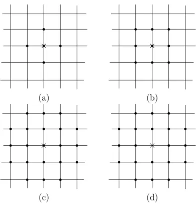
Take S+≡ S = Z2, G the 4-nearest neighbours graph, C = {3i, i ∈Z2}, V i =
{j ∈ Z2 : ki − jk
1 ≤ 1}. In this case P = {Wi, i ∈ C} where Wi = {j ∈Z2 :
ki − jk∞ ≤ 1} is a CSP and W∗
i = {j ∈Z2 : ki − jk1 ≤ 3 and ki − jk∞≤ 2}
(see Figure 1). For Λn = [−n, +n]2 and Cn = C ∩ Λn, the asymptotic rate,
lim infn→∞ |C|Λnn||, is positive and equal to 19.
Regular lattice
Z
2with holes and nearest neighbours
graph
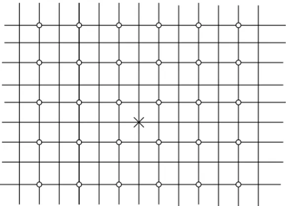
Let T = (1, 1) + 2 × Z2 the holes set, S =Z2\T, S+ = Z2, C = 6 ×Z2 (see
(a) (b)
(c) (d)
Figure 1: (a) Neighbourhood Vi of site i (×) for the 4-nearest neighbours, (b)
second order neighbourhood (Moore neighbourhood) Wi, (c) neighbourhood
W∗
i and (d) neighbourhood Ui.
nearest neighbours graph: two thirds of the sites have 2-nearest neighbours whereas one third have 4-nearest neighbours. P = {Wi, i ∈ C} is a CSP if
we take Wi = {j ∈ S : ki − jk∞ ≤ 1}. For Ui = Wi∗\{i}, there are three
types of (Wi, Wi∗, Ui), namely
1. If i ∈ (0, 0)+6×Z2, W
i, Wi∗and Ui contain 5, 9 and 8 sites respectively
(see Figure 3);
2. for i ∈ (3, 0) + 6 ×Z2, or i ∈ (0, 3) + 6 ×Z2, W
i, Wi∗ and Ui contain 7,
13 and 12 sites (see Figure 4); 3. for i ∈ (3, 3) + 6 ×Z2, W
i, Wi∗ ≡ Ui contain 8 and 16 sites (see Figure
5).
Figure 2: Regular lattice with holes (◦).
(a) (b) (c)
Figure 3: (a) Neighbourhood Wi, (b) neighbourhood Wi∗, (c) neighbourhood
Ui for i ∈ (0, 0) + 6 ×Z2.
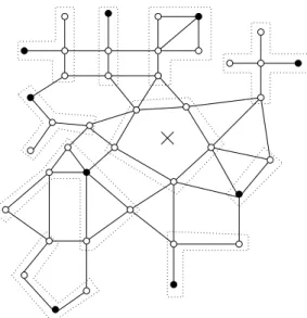
A finite and irregular lattice
S
This example deals with a finite and irregular lattice S with 41 sites (◦ and •) and a graph defined as in Figure 6. We take S+ = S ∪{×} and we consider
C with 10 points (•) and the point ×. Note that C * S. Then the partition P = {Wi, i ∈ C}, where Wi is delimited by the dotted lines, is a CSP. The
partition rate is equal to 9 42.
Given a CSP P we can rearrange the terms of Sn as
Sn= X i∈Λn Yi = X i∈Cn X j∈Wi,n Yj = X i∈Cn Gi,n
where Cn = {i ∈ C : Wi,n 6= ∅}, Wi,n = Wi ∩ Λn and Gi,n =
P
j∈Wi,nYj.
(a) (b) (c)
Figure 4: (a) Neighbourhood Wi, (b) neighbourhood Wi∗, (c) neighbourhood
Ui for i ∈ (3, 0) + 6 ×Z2.
(a) (b)
Figure 5: (a) Neighbourhood Wi, (b) neighbourhood Wi∗ ≡ Ui for i ∈ (3, 3)+
6 ×Z2.
the partial sums Gi,n.
Lemma 1 For two different sites of C , l and k, Gl,n and Gk,n are
condi-tionally independent with respect to FC.
Thus we have
Var(Sn/FC) =
X
i∈Cn
Var(Gi,n/FC). (7)
According to (6), a strategy for verifying (N 3) consists in three steps :
1. bounding from below Var(Gi,n/FC), i ∈ C;
2. bounding from below EFC(Var(Gi,n/FC));
Figure 6: An example of irregular finite lattice.
Step 3 is purely combinatorial and requires a direct examination of G and S+. For the other steps, it is sufficient to look at points i ∈ C provided that
|∂Λn|/|Λn| −→ 0. We can also restrict our investigation to points i ∈ C ∩ S
since, if i /∈ S, then Gi,n is FC-constant.
Thus we focus on i ∈ C ∩ S such that i /∈ ∂Λn. In this case, we have
(Gi,n/FC) = gi(Xi, xUi). No universal tools are available for bounding
gen-eral expressions of Var(Gi,n/FC) from below. This variance is positive
pro-vided that (Gi,n/FC) is not constant; therefore we have to find xUi such
that (Gi,n/FC) is not constant. We need only study minorizations for sites
i ∈ C1 ⊂ C∩S provided lim infn→∞|C1,n| / |Cn| = κ > 0, with C1,n= C1∩Λn.
In some cases, we can choose C1 such that the geometry of Ui does not
de-pend on i ∈ C1 and πUi(·/xUi) is bounded from below by c× π(·/xUi), where
c is a strictly positive constant and π(·/xUi) only depends on xUi.
For the second step, note that
EFC(Var(Gi,n/FC)) =
Z
Var(Gi,n/xU)πU(xU)λ(dxU).
A bound for this expression is obtained when πU is bounded from zero and
Var(Gi,n/xU) is positive over a set of xU with positive measure. If the
(xU, x∂U), we have
πU(xU) =
Z
πU(xU/x∂U)π∂U(x∂U)λ(x∂U) ≥ ρ
Z
π∂U(x∂U)λ(x∂U) = ρ
with ρ = infxU,x∂U πU(xU/x∂U) > 0.
5
Examples
5.1
Isotropic Ising model in a random environment on
Z
2Let S =Z2, p > 0 a positive probability and G(p) the percolation graph on S
defined as follow : let L = {Li,j, i, j ∈ S, ki − jk1 = 1} be a collection of
in-dependent identically distributed Bernoulli random variables with parameter p; then, for each i ∈ S, the neighbourhood of i is
∂i = {j ∈ S s.t. ki − jk1 = 1 and Li,j = 1}
An nearest neighbourhood Ising model for this graph is a probability π on {−1, +1}Z2 such that πi(xi | xi) = πi(xi | x∂i) = exp{xi(α + βvi)} 2 cosh(α + βvi) (8) where vi =Pj∈∂ixj.
For p = 1, this is the 4-nearest neighbour Ising model and for some val-ues of θ = (α, β), there are more than one probability satisfying (8) (Georgii, [10]). This causes difficulties in studying asymptotic properties of local esti-mators like maximum pseudo-likelihood estimator (MPLE), coding estimator (see Comets [5] and Guyon [11]). For 0 < p < 1, the graph is not regular and potentials are not shift invariant.
Assume that X is observed on the neighbourhood Λ∗n of Λn = [−n, +n]2
and we concentrate on MPLE ˆθ, a maximiser of the logarithm of the pseudo-likelihood
Un(θ) =
X
i∈Λn
Derivation of asymptotic normality for ˆθ involves examination of asymptotic properties of the derivative of Un
Un(1)(θ) = X i∈Λn (log πi)(1)(xi | xi; θ) = X i∈Λn ¡1 vi ¢ (Xi− tanh(α + βvi)).
If we consider Yi = (a + bvi)(Xi− tanh(α + βvi)), (a, b) 6= 0, then Yi satisfies
(2). More generally, for some non zero function b, we prove the CLT for the sum of conditionally centred functional
Yi = b(vi)(Xi− tanh(α + βvi))
To verify (N 3), choose C = 3 ×Z2, W
i = {j : kj − ik∞ ≤ 1} : P =
{Wi, i ∈ C} is a CSP of S. Define, for (Vi)∗ the second order neighbour of i,
C1 = {i ∈ C s.t. Lk,l = 1 if k, l ∈ (Vi)∗ and kk − lk1 = 1}
C1 is the subset of C of site i such the 16 pairs of nearest neighbour sites of
(Vi)∗ are all connected. It is easy to see that
lim n |C1,n| |Λn| = p 16 9 > 0 We have Var(X i∈Λn Yi) ≥ X i∈Cn E{Var(Yi+ X j∈Wi,n\{i} Yj | FC)}.
Look at sites i ∈ C1∩ [−(n − 2), (n − 2)]2. As (Vi)∗ ⊆ Λn, we have
Yi+
X
j∈Wi\{i}
Yj = Gi(Xi, xAi) + gi,
where gi is FC-constant and Ai = i + A0 where A0 = {j ∈ S : kjk1 = 1 or
2}.
For i ∈ C1, b : V → R with V = {−4, −2, 0, 2, 4}. Suppose that b is
not zero. The crucial functional step in Guyon and K¨unsch [13] (see Proof of Theorem 3, page 190-193) is still valid here, without any hypothesis of shift invariance, stationarity or ergodicity for the Ising model. This result is the following there exists a configuration x0A0 on A0 such that, uniformly in
i ∈ C1,n, Xi 7→ Gi(Xi, x0Ai) is not constant, x
0
Ai being the configuration x
0 A0
shifted from i. Then, according to (8), (Xi | x0Ai) is not constant and there
exists δ > 0 such that, for every i ∈ C1,n, Var(Yi+PWi\{i}Yj | FC) ≥ δ > 0.
Therefore, E(Var(Yi+
P
Wi\{i}Yj | F
C)) ≥ δ × π(x0
Ai). On the other hand, a
bound from below for π(x0
Ai) is a consequence of Bayes formula:
π(xAi) =
X
x∂Ai
π(xAi | x∂Ai)π(x∂Ai) ≥ ε
where ε = infyAi,y∂Aiπ(yAi | y∂Ai) > 0. Thus we have, for large n,
Var(Sn) ≥ p16×
δ × ε
10 × |Λn| .
For p = 0, CLT is trivial because the random variables Yiare independent
and identically distributed. For p = 1, we are in presence of the 4-nearest neighbour. Ising model (Guyon and K¨unsch, [13]): CLT for Y is valid re-gardless of phase transition, or non stationarity, or non ergodicity of the model.
The result obtain here for the percolation graph can be generalized to more general random environment : the main property of the random graph that is need is the sub-ergodicity of the subset C1 : lim infn|C|C1nn|| > 0.
5.2
Isotropic Ising model on
S =
Z
2\
T
Consider the non-stationary nearest neighbours isotropic Ising model on S = Z2\T, T = (1, 1) + 2 × Z2, Λ
n= [−n, +n]2∩ S, and the centred functional
Yi = b(vi)(Xi− tanh(α + βvi))
with vi = Pj∈∂ixj. Take the CPS as defined in example 2. If we focus on
C1 = (3, 0) + 6 ×Z2, (N3) is fulfilled and limn→∞ |C|Λ1,nn|| = 271. For i = (3, 0),
Yi +
P
Wi\{i}Yj = Gi(Xi, xAi) + gi, where gi is F
C-constant, and A
i = {j ∈
S : kj − ik1 = 1 or 2, j 6= (3, ±1) and j 6= (3, ±2)}. We can show that there exists xAi such that x 7→ Gi(x, xAi) is not constant and we can apply same
argument as before to prove CLT for Y .
5.3
Ising model on an irregular lattice
Consider S is an infinite countable set equipped with a graph G satisfying (N 2). Suppose also that there exists a CPS, P = {Wi, i ∈ C}, with basis
(S, C) such that for every i, Vi = {i} ∪ ∂i ⊂ Wi. Suppose that (Λn) is a
strictly increasing sequence such that lim infn |C|Λnn|| > 0.
Let X be an Ising model on (S, G) with conditional laws
for i ∈ S : πi(xi | x∂i) =
exp{xi(αai+ βvi)}
2 cosh(αai+ βvi)
, (9)
where vi = Pj∈∂ibijxj, θ = (α, β) is a parameter and (ai), (bij = bji) are
known weights. The conditionally centred functional Y is Yi = bi(x∂i)(Xi− tanh(αai+ βvi)
and Sn =Pi∈ΛnYi =Pi∈CnGi,n.
If i ∈ C and (Vi)∗ ⊂ Λn, Gi,n = Gi = Gi(Xi, x∂i∪∂2i) + gi where gi is
FC-constant, ∂2i = {k, k 6= i : ∃j ∈ ∂i s.t. k ∈ ∂j}, and
Gi(Xi, xAi) = bi(x∂i)Xi+
X
j∈∂i
bj(Xi, wj,i){xj − mj(Xi, wj,i)}
where, for j ∈ ∂i, wj,i = (xk, k ∈ ∂j\{i}). We can verify (N3) by the
following steps:
1. find C1 ⊂ C such that:
(a) lim infn |C|C1,nn|| > 0;
(b) for each i ∈ C1, ∃x∂i∪∂2is.t. ∆i = Gi(+1, x∂i∪∂2i)−Gi(−1, x∂i∪∂2i) 6=
0;
(c) get a uniform lower bound for |∆i| over C1;
2. get a uniform lower bound for πi(xi | x∂i) and π∂i∪∂2i(x∂i∪∂2i) in i ∈ C1,
xi, x∂i, x∂i∪∂2i.
Step 1 requires ad hoc strategies. Step 2 follows easily provided (ai) and
(bij) are bounded since conditional probabilities are positive and continuous
in (ai, bij), xi, x∂i and x∂i∪∂2i.
Now we consider Yi = (avii)(Xi− tanh(αai+ βvi)). To prove CLT for (Yi),
we need only to consider linear real functions bi(vi) = aai+ bvi, (a, b) 6= 0.
Setting, for j ∈ ∂i, vj,i = vj− bi,jxi = Pk∈∂j\{i}bk,jxk, we can write
∆i = gi(x∂i; a, b) + hi(x∂2i, a, b; θ), with gi(x∂i) = 2bi(vi) and
hi(x∂2i) = −
X
ξ∈{−1,+1}
X
j∈∂i
To simplify, look at the particular case where ∂i ∩ ∂2i = ∅ for any i ∈ C 1.
1. If b 6= 0, for any x∂2i , ∆itakes two values ∆′
i 6= ∆′′i provided there exists
two configurations x′∂iand x′′∂isuch that vi′ 6= v′′i. As max{|∆′i| , |∆′′i|} ≥ 1
2|b| |v ′
i− vi′′|, we have a lower bound for |∆i| if we can obtain a lower
bound for |v′ i− vi′′|.
2. If b = 0, then ∆i = aaiDi(x∂2i) where Di(x∂2i) = (2−P
j∈∂itanh(αaj−
βbi,j + βvj,i) − tanh(αaj + βbi,j + βvj,i). Then (N3) holds under the
conditions : inf i∈C∗ 1 |ai| > 0 and inf i∈C∗ 1 sup x∂2i |Di(x∂2i)| > 0.
An irregular lattice which comes from a Poisson process on R
Now we shall consider a particular example of irregular lattice. Suppose that S is a realisation of an homogeneous Poisson process on R, and write S = {ik, k ∈Z} with ik< il if k < l. Consider the 2-nearest neighbour Ising
model on S, with weight ai ≡ 0 and bi,j = f (|i − j|) for f : (R+)∗ −→ (R+)∗
decreasing.
For C = {i3k, k ∈ Z} and Wik = {ik−1, ik, ik+1}, the partition P =
{Wi, i ∈ C} is a CSP. Define
C1 = {il ∈ C : inf{|il− il−1| , |il− il+1|} ≤ 1}
and Λn= [−n, +n] ∩ S. It is easy to verify that limn |C|Λ1,nn|| > 0.
On the other hand, because vil = bil,il−1xil−1 + bil,il+1xil+1, the range of
variation of vil is eil = 2(bil,il−1 + bil,il+1) and infi∈C1ei > 0. Thus (N3) is
satisfied.
Note that we can weaken the hypothesis about the Poisson process, in-cluding dependence and/or inhomogeneity for other point processes.
5.4
Gaussian MRF on a irregular lattice
Let X be a Gaussian MRF on (S, G). The conditional law in each site is Xi|x∂i ∼ N (αvi, wi) (10)
where wi > 0, vi =
P
j∈∂ibijxj (ai, bij) are known weights, α is an unknown
We set ai = w−1i . The conditional specification (10) is coherent if for any
i, j ∈ S, i 6= j, aibij = ajbji and for any finite subset Λ ⊂ S, the symmetric
matrix JΛ = (JΛ(i, j))i,j∈Λ, where JΛ(i, i) = ai, JΛ(i, j) = −αaibij, i, j ∈ Λ,
i 6= j, is positive definite.
If X is observed on a increasing sequence (Λn) of S, asymptotic normality
of MPLE bαn can be proved under the contraction condition (Guyon, [11,
Section 4.3]) : |α| {sup i X j∈∂i |bij|} < 1 (11)
This condition entails that there is not phase transition and X is α-mixing (Doukhan, [9]). The last property allow us to establish the asymptotic nor-mality.
We prove asymptotic normality of MPLE bαn by means of proposition
1 without condition (11). The verification of condition (N3) still requires careful examination. The conditionally centred functional Y is
Yi = (log π(xi | x∂i)(1)α = aivi(Xi− αvi).
Let P = {Wi, i ∈ C} be a PCS with C ⊆ S such that for any i, Vi =
{i} ∪ ∂i ⊆ Wi. For all (Vi)∗ ⊆ Λn we have
Gi,n= Gi = aivi(Xi− αvi) +
X
j∈∂i
ajvj(xj− αvj) + gi
where gi is FC(X)-constant. For j ∈ ∂i, we denote vj = bjiXi + vji with
vji =
P
k∈∂j,k6=ibjkxk. We can also write Gi as:
Gi = ciXi+ dijXi2+ eij
where ci =Pj∈∂iajbij(xj − 2αvji) and dij = −α{Pj∈∂iajb2ij}. Note that ci,
dij and eij are FC(X)-constant.
A lower bound for V ar(Gi | FC(X)) is determined by noting that if
Z ∼ N (µ, σ2), and G = cZ + dZ2 then V ar(G) = (c + 2dµ)2σ2+ 2d2σ4 ≥ 2d2σ4. We obtain V ar(Gi | FC(X)) ≥ 2α2{ X j∈∂i ajb2ij}2× a−2i = 2α2{ X j∈∂i bij× bji}2.
The lower bound does not depend on x∂i, thus a sufficient condition for (N3)
is
α 6= 0 and lim inf
n P i∈Cn{ P j∈∂ibij × bji}2 |Λn| > 0.
References
[1] Besag, J., 1974. Spatial interaction and the statistical analysis of lattice systems. Journal of the Royal Statistical Society, series B 36, 192–236. [2] Bolthausen, E., 1982. On the central limit theorem for stationary mixing
random fields. Annals of Probability 10, 1047–1050. [3] Breiman, L., 1992. Probability. SIAM.
[4] Cliff, A. D., Ord, J. K., 1981. Spatial Processes: Models and Applica-tions. Pion Ltd.
[5] Comets, F., 1992. On consistency of a class of estimators for exponential families of Markov random fields on the lattice. The Annals of Statistics 20, 455–468.
[6] Comets, F., Janzura, M., 1998. A central limit theorem for conditionally centered random fields with an application to markov fields. Journal of Applied Probability 35, 608–621.
[7] Cressie, N., 1991. Statistics for Spatial Data. Wiley, New York.
[8] Dedecker, J., 1998. A central limit theorem for stationary random fields. Proba. Theory Relat. Fields 110, 397–437.
[9] Doukhan, P., 1994. Mixing: Properties and Examples. Lecture Notes in Statistics 85, Springer, New York.
[10] Georgii, H.-O., 1988. Gibbs Measures and Phase Transitions. Walter de Gruyter and Company.
[11] Guyon, X., 1995. Random Fields on a Network. Springer, New York. [12] Guyon, X., Hardouin, C., 2001. Markov field dynamics : models and
[13] Guyon, X., K¨unsch, H. R., 1992. Asymptotic comparison of estimators in the Ising model. In: Lecture Notes in Statistics. Vol. 74. Springer, Berlin, pp. 177–198.
[14] Haining, R., 1990. Spatial Data Analysis in the Social and Environmen-tal Sciences. Cambridge University Press, Cambridge.
[15] Jensen, J., K¨unsch, H. R, 1994. On asymptotic normality of pseudo-likelihood estimation for pairwise interaction processes. Annals of the Institute of Mathematical Statistics 46, 475–486.
[16] Stein, C., 1973. A bound for the error of normal approximation of a sum of dependent random variables. In: Proc. Sixth Berkeley Symp. Math. Statist. Prob. Vol. 2. pp. 583–602.
[17] Tiefelsdorf, M., 2000. Modelling Spatial Processes. Lecture Notes in Earth Sciences Vol. 87. Springer, Berlin.