Energy Accounting and Control with SLURM Resource and Job Management System

(1)

HAL Id: hal-01237596

https://hal.inria.fr/hal-01237596

Submitted on 3 Dec 2015

HAL is a multi-disciplinary open access

archive for the deposit and dissemination of

sci-entific research documents, whether they are

pub-lished or not. The documents may come from

teaching and research institutions in France or

abroad, or from public or private research centers.

L’archive ouverte pluridisciplinaire HAL, est

destinée au dépôt et à la diffusion de documents

scientifiques de niveau recherche, publiés ou non,

émanant des établissements d’enseignement et de

recherche français ou étrangers, des laboratoires

publics ou privés.

Energy Accounting and Control with SLURM Resource

and Job Management System

Yiannis Georgiou, Thomas Cadeau, David Glesser, Danny Auble, Morris

Jette, Matthieu Hautreux

To cite this version:

Yiannis Georgiou, Thomas Cadeau, David Glesser, Danny Auble, Morris Jette, et al.. Energy

Ac-counting and Control with SLURM Resource and Job Management System. ICDCN 2014, Jan 2014,

Coimbatore, India. �10.1007/978-3-642-45249-9_7�. �hal-01237596�

(2)

Energy Accounting and Control with

SLURM Resource and Job Management System

Yiannis Georgiou1, Thomas Cadeau1, David Glesser1,

Danny Auble2, Morris Jette2, Matthieu Hautreux3

1 BULL S.A.S Yiannis.Georgiou|Thomas.Cadeau|David.Glesser@bull.net 2 SchedMD {da}|{jette}@schedmd.com 3 CEA DAM Matthieu.Hautreux@cea.fr

Abstract. Energy consumption has gradually become a very important parameter in High Performance Computing

platforms. The Resource and Job Management System (RJMS) is the HPC middleware that is responsible for distribut-ing computdistribut-ing power to applications and has knowledge of both the underlydistribut-ing resources and jobs needs. Therefore it is the best candidate for monitoring and controlling the energy consumption of the computations according to the job specifications. The integration of energy measurment mechanisms on RJMS and the consideration of energy con-sumption as a new characteristic in accounting seemed primordial at this time when energy has become a bottleneck to scalability. Since Power-Meters would be too expensive, other existing measurement models such as IPMI and RAPL can be exploited by the RJMS in order to track energy consumption and enhance the monitoring of the executions with energy considerations.

In this paper we present the design and implementation of a new framework, developed upon SLURM Resource and Job Management System, which allows energy accounting per job with power profiling capabilities along with parameters for energy control features based on static frequency scaling of the CPUs. Since the goal of this work is the deployment of the framework on large petaflopic clusters such as CURIE, its cost and reliability are important issues. We evaluate the overhead of the design choices and the precision of the monitoring modes using different HPC benchmarks (Linpack, IMB, Stream) on a real-scale platform with integrated Power-meters. Our experiments show that the overhead is less than 0.6% in energy consumption and less than 0.2% in execution time while the error deviation compared to Power-meters less than 2% in most cases.

1 Introduction

Energy Consumption is playing a very significant role in the evolution of High Performance Computing Platforms. The increase in computation performance of Supercomputers has come with an even greater increase in energy consumption, turning energy an undisputted barrier towards the exascale. Research efforts upon all different abstraction layers of com-puter science, from hardware, to middleware upto applications, strive to improve energy conservations. The advances on hardware layer need to be followed by evolutions on systems software and middleware in order to achieve important results.

As far as the systems middleware concerns, the Resource and Job Management System (RJMS) can play an important role since it has both knowledge of the hardware components along with information upon the users workloads and the executed applications. Energy consumption is the result of application computation hence it should be treated as a job characteristic. This would enable administrators to profile workloads and users to be more energy aware. Furthermore power consumption analysis with timestamps would enable users to profile their applications and perform optimizations in their code. Hence the first step that needs to be made is to measure power and energy through the RJMS and map them to jobs. Introducing Power-Meters on Supercomputers would be too expensive in terms of money and additional energy hence using the already available interfaces seemed the most viable approach.

This paper presents the design and evaluation of energy accounting and control mechanisms implemented upon the SLURM Resource and Job Management System. SLURM [1] is an open-source RJMS specifically designed for the scal-ability requirements of state-of-the-art supercomputers. In Junes’ 2013 Top 500 list [2] SLURM was the default RJMS of 5 supercomputers in the top 10. The new framework allows power and energy consumption monitoring per node and accounting per job based on IPMI and RAPL measuring interfaces. The new monitoring modes are enhanced with mech-anisms to control energy consumption based on static frequency scaling of the CPUs, allowing users to experiment on the

(3)

trade-offs between energy consumption and performance. The new features presented in this paper are currently in the latest 2.6 version of SLURM released on July 2013.

Having as goal the deployment of the framework on large petaflopic clusters such as the French PRACE Tier0 system

CURIE1_{, its cost and reliability are important issues. We perform experimentations of the new framework upon a}

real-scale platform with integrated Power-Meters and we evaluate the overhead of the monitoring modes and the precision of the power and energy data during the executions of different HPC applications (Linpack, IMB, Stream).

The remainder of this article is presented as follows: The next section provides the Background and Related Work upon power and energy monitoring and power management for RJMS. Section 3 describes the new framework. In Section 4 we present and discuss our evaluation results upon the overhead and precision of the new energy monitoring framework. Finally, the last section presents the conclusions along with current future directions.

2 Background and Related Work

The best approach to accurately track power and energy consumption data in HPC platforms would be to use dedicated devices such as power-meters [3] for the collection of the power of the whole node or devices like PowerInsight [4] and PowerPack [5] for power consumption of node’s individual components. In more detail the PowerPack framework [5] consists of hardware sensors for power data collection and software components to use those data for controlling power profiling and code synchronization. Nevertheless, the usage of additional hardware on large HPC clusters would be too expensive therefore the alternative to exploit built-in interfaces seemed more viable for now.

The Intelligent Platform Management Interface [6] is a message-based, hardware-level interface specification concieved to operate even independently of the operating system in an out-of-band function. It is used by system administrators mainly to perform recovery procedures or monitor platform status (such as temperatures, voltages, fans, power consumption,etc) The main intelligence of IPMI is hidden on the baseboard management controller (BMC) which is a specialized micro-controller embedded on the motherboard of a computer which collects the data from various sensors such as the power sensors. The advantage of IPMI is that it can be found in nearly all current Intel architectures and if power senosrs are

supported it can provide a very cheap built-in way for power collection. Various opensource software23exist for in-band

and out-of-band collection of IPMI sensors data. Hackenberg et al. in [7] show that the power data collected from IPMI are sufficiently accurate but the calculation of energy consumption might not be precise for jobs with small duration. In

the evaluation section we argue that this might not be the case with newer architectures and BMC. Collectl4_{is a system}

monitoring tool that tracks various sensors, amongst which the power, through in-band IPMI using ipmitool1_{. The data}

are stored in a compressed format per node basis.

The Running Average Power Limit (RAPL) interface has been introduced with the Intel Sandy Bridge processors [8] and exists on all later Intel models. It provides an operating system access to energy consumption information based on a software model driven by hardware counters. One of the specificities of the model is that it tracks the energy consumption of sockets and DRAM but not that of the actually memory of the machine. Various articles have been published that use RAPL to measure energy consumption within systems [9],[10] and they have all reported reliable results. PAPI [11] performance profiling tool provides the support of monitoring energy consumption through RAPL interfaces.

Unfortunately RAPL model reports energy on the level of socket and not on the level of core. However, model-based power estimates [12] have shown to be fairly precise, opening the way for near future support of core based power consumption on hardware and software.

High resolution power profiling would allow application performance tools to correlate them with MPI traces, hardware performance counters and other performance metrics. Hence having this data in OTF2 format [13] would allow a scenario like this. Nevertheless in the context of real-time power profiling through a Resource and Job Management system high resolution might increase the overhead which will have a direct interference to the application execution. In this context usage of binary files such as the Hierarchical Data Format v5 (HDF5) [14],[15] would provide a more viable approach. Various Resource and Job Management Systems such as MOAB, PBSPro and Condor advertise Power Management techniques especially based on exploitation of idle resources. LoadLeveler which is a proprietary software seems to be

one of the first to provide power and energy monitoring5_{along with energy aware scheduling based on automatic CPU}

Frequency setting by the system according to a prediction model. LoadLeveler with those energy aware features is used

1 http://www.prace-ri.eu/CURIE-Grand-Opening-on-March-1st-2012?lang=en 2_{http://ipmitool.sourceforge.net/} 3 http://www.gnu.org/software/freeipmi/ 4 http://collectl.sourceforge.net/ 5 http://spscicomp.org/wordpress/pages/energy-aware-scheduling-for-large-clusters/

(4)

on SuperMUC supercomputer in LRZ. Hennecke et al. present the retrieval of power consumption data from IBM Blue Gene/P supercomputer [16] through a particular LoadLeveler tool called LLview. In addition, LLview has the capability to provide power consumption data per job basis in high precision with about 4 samples per second. Nevertheless, this tool is closed source and specifically developed for BlueGene/P platforms.

One common mechanism on newer microprocessors is the mechanism of on the fly frequency and voltage selection, often called DVFS. Reducing CPU frequency may lead in energy reductions. Various strategies, using DVFS technique, have been widely studied to improve the energy consumptions of MPI applications [17],[18]. Other studies have shown that adaptive usage of frequency scaling may result in important energy benefits for small performance losses [19]. The control of energy consumption through CPU Frequency scaling as a user feature was initially studied and implemented on OAR [20] which is another flexible RJMS for HPC clusters.

3 Integrating power/energy consumption retreival and control on SLURM

SLURM has a particular plugin dedicated on gathering information about the usage of various resources per node during job executions. This plugin, which is called jobacct gather, collects information such as CPU and Memory utilization of all tasks on each node and then aggregates them internally across all nodes and returns single maximum and average values per job basis.

Controller Computing Nodes

slurmctld slurmd slurmd _... slurmd

Database slurmdbd Client Cluster Hardware SLURM Permanent SLURM Job Related

slurmstepd slurmstepd slurmstepd srun salloc sbatch SLURM Jobacct_gather Acct_gather_Energy IPMI Acct_gather_Energy RAPL Acct_gather_Profile HDF5 ... ... ... No Threads jobacct ipmi profile Basic Monitoring Extended Monitoring Power/Energy Data Movement Internal RPC Power/Energy Data Collection jobacct jobacct ipmi ipmi profile profile sstat scontrol sacct Threads Threads Threads Processes Deamons Commands and

hdf5 file hdf5 file hdf5 file

i) ii) iii) iv) v) vi)

Fig. 1.SLURM Monitoring Framework Architecture with the different monitoring modes

Resource utilization collection was already supported in SLURM. The goal of our new developments was to extend this mechanism to gather power and energy consumption as new characteristics per job. Of course, as we will see in this section, only per job energy consumption is stored in the SLURM database. Instant power consumption needs to be stored in relation with timestamps and thus a different model is used. This section is composed by 5 parts. Initially we describe the whole framework design of the new monitoring modes, then RAPL dedicated mode is presented, followed by the subsection for IPMI mode. Subsection 3.4 describes how power profiling with HDF5 is implemented and finally the last part describes the function of setting the CPU Frequency for controlling the energy consumption.

3.1 SLURM Monitoring Framework Architecture

We will begin by delving a bit more into the details of SLURM’s architecture of the monitoring mechanisms. Figure 1 shows an overview of SLURM’s deamons, processes and child threads as they are deployed upon the different components of the cluster. In the figure the real names of deamons, processes and plugins have been used (as named in the code) in order to make the direct mapping with the code. In SLURM architecture, a job may be composed by multiple parallel sub-jobs which are called steps. A job is typically submitted through the sbatch command with the form of a bash script. This script may contain multiple invocations of SLURM’s srun command to launch applications (sub-jobs) in parts or the entire job allocation as specified by sbatch. To simplify the explanation let us consider the simpler case of job with one step. When this job is launched, the srun command will be invoked on the first node of job allocation and the slurmd deamons will launch a slurmstepd process on each node which will be following the execution of the whole step (shown by latin number ii) in figure 1).

If the basic monitoring mode is activated the jobacct gather plugin is invoked and the slurmstepd process will launch a thread upon each node that will monitor various resources (CPU, Memory, etc) during the execution (as shown by iii)

(5)

in Figure 1). The polling of resources utilization is done through Linux pseudo-file system /proc/ which is a kernel data structure interface providing statistics upon various resources in the node. The sampling frequency is user specified on job submission. The various statistics are kept in data structures during the execution and aggregated values upon all nodes (Average,Max, etc) are stored in the database when the job is finished. The data are moved between threads and processes with internal RPC keeping the mechanism reliable and efficient. These information can be retrieved by the user during the execution of the job through the SLURM command sstat and after its termination through sacct.

The new monitoring modes will follow the same design architecture with seperate plugins for each monitoring mode and launching of new threads to keep their polling asynchronous with the basic monitoring mode.

3.2 Power data collection through IPMI interface

There are various opensource software to support the IPMI protocol and enable the retrieval of power data from the BMC:

Ipmitool6, OpenIPMI,etc. Our choice was to select freeipmi7for various reasons, it is dedicated to HPC, it does not need

kernel modules and it provides an easily integrated API. One important difference between IPMI and RAPL retrieval is the duration of the call. The call would usually take from 4ms up to 80ms but sometimes the call could take more than 2 or 3 sec. Hence we needed to turn the collection asynchronous to the tracking of the rest of the resources and the job control of execution. So a seperate thread was required to deal with the IPMI call. Furthermore we wanted to communicate to this thread not only from the jobacct thread during the execution of the job but also from the slurmd in order to get information about the power consumption of the node for system information.

Hence the choice was to launch the IPMI polling thread from slurmd as we can see on figure 1 with the latin number iii) the IPMI threads have the same color as the slurmd processes. An important issue here is that IPMI collects power in watts and we are interested to calculate the energy consumption of the job. Hence a particular algorithm needs to be used initially to calculate energy consumption per node and then aggregate that for all the allocated nodes to obtain the energy consumption per job. The sampling frequency is fixed with a particular option defined by the administrator for

each node. A sleep function inside the thread allows to add energy depending on this frequency dt. Let’s consider tn a

polling time, then the next polling time would be tn+1= tn+ dt. We need to note that times are computed using the C

function ”time(NULL)”, which is in seconds. thus the difference tn+1− tn which will take values in dt− 1, dt, dt + 1

would always be in seconds. Considering that the corresponding power values for the above times would be wnand wn+1,

the energy consumption dEnbetween tnand tn+1is computed from the following equation upon each node:

dEn= (tn+1− tn)×

wn+ wn+1

2 (1)

This formula is used to add the energy consumption dEnto the total energy EN used since the node has started.

To deduce the energy consumption for the job per node we take the difference between the consumed energy of the node

on the start of the job and the respective energy at the time the job has terminated ENjob = EN (start)− EN(stop)

Finally the sum of the energies on each node as calculated from the above equation would give us the energy consumption of the job. Ejob= K X k=0 ENjob(k) (2)

The energy data are communicated between the IPMI thread towards jobacct thread and slurmd using internal Remote Procedure Calls. The instant power data are communicated with another RPC towards the profile thread if profiling is activated, as show us the red arrows in Fig.1.

3.3 Energy data collection from RAPL model

As we show in section 2 RAPL model returns energy consumption value representing the energy consumed since the boot of the machine. Having energy data directly simplifies the procedure for the calculation of the energy consumption of the whole job but complexifies the power consumption profiling. The collection of energy data is made through the particular Linux MSR driver following the technique described here. The actual call for data retrieval is really fast about 17µs. In addition, the collection of only 2 energy data per node are sufficient for the calculation of the energy consumption of the entire job (one in the beginning and on in the end of the job). The final energy consumption of the job on one node will be

6

http://ipmitool.sourceforge.net/

7

(6)

the difference of the energy in the end and that in the start. Finally, adding the energies calculated on each node will give us the energy consumption of the entire job.

Based on the fact that the actual call to RAPL is fast and the fact that we do not need seperate sampling there is no need to have a particular thread responsible for collecting the energy data on each node (as shown on Fig.1 with latin number v) ). Hence the dedicated functions of the acct gather energy RAPL plugin collect data from the RAPL model whenever they are asked and transfer those data through internal RPC (red arrows in Fig.1) towards the demanding threads or processes. The calculation of instant power consumption per node can be calculated by collecting 2 samples of energy and dividing their difference by the frequency of the sampling. Hence a parameter has been defined to allow the adiministrator to provide this frequency in order to be able to extract power consumption through the RAPL energy data. Currently the choice has been to set this frequency no less than 1sec. However, as explained by Hackenberg et al. in [7], the precision of the power data is directly dependent on the actual sampling of RAPL internally which is about 10ms. We believe that allowing lower sampling might increase the overhead and we wanted to make evaluations before allowing something like that. Hence, initially our choice was to loose a little bit in precision but gain in terms of overhead.

3.4 Power data Profiling with hdf5 file format

Energy consumption is a global value for a job so it is obvious that it can be stored in the database as a new job characteris-tic. However, power consumption is instantaneous and since we are interested to store power consumption for application profiling purposes; a highly scalable model should be used. Furthermore since the application profiling will also contain profiling statistics collected from various resources (like network, filesystem, etc), a mechanism with extensible format would be ideal to cover our needs.

Hence a new plugin has been created called acct gather profile, presented by latin number vi) in Fig.1. This plugin is responsible for the profiling of various resources. Apart energy profiling, network, filesystem and tasks profiling is sup-ported but the analysis of these types goes beyond the purposes of this paper. As we can see in the graphic representation of Fig.1 the profile thread is launched from slurmstepd (same color) and it collects the power and energy consumption data from IPMI thread or RAPL functions through internal RPC. The collected data are logged on hdf5 files per node. Ideally the storage of these files should be made upon a shared filesystem in order to facilitate the merging of files after the end of the job. The profiling information cannot be retrieved by the user during the execution of the job and this is because the hdf5 files are binaries which are readable only after the job termination.

The sampling frequency is an important parameter of profiling and the choice of implementation was to allow users to provide the particular frequency they need for each different type of profiling. Currently the lowest possible sampling frequency is 1 second, which according to other studies is long for the RAPL case, where the sampling frequency should be around 1ms in order to obtain the highest precision possible. Nevertheless we argue that having a thread polling 1000 samples per second would probably introduce a large overhead and we wanted to be sure about the overall overhead and precision with 1 sample per second before we try to optimize the measurements.

So during the execution of the job, each profile thread creates one hdf5 file per node and at the end of the job a merging phase takes place where all hdf5 files are merged into one binary file, decreasing the actual profile size per job. The profiling takes place only while the job is running, which is a big advantage opposed to other profiling techniques such as collectl where the profiling is continuous resulting in enormous volume of data that is not even correlated to jobs.

3.5 Control Static CPU Frequency Scaling

Giving the possibility to users to account power and energy consumption per job is an interesting feature but it would be limited if they don’t have a way to control it. One method that is used a lot to control energy consumption, both in modeled and practical studies, is the CPU Frequency Scaling. Based on particular Linux kernels features we have provided the support of static CPU Frequency Scaling through a newly introduced parameter in srun command. The implementation passes from cgroups or cpusets in order to track the exact cores that the application is being executed and the actual setting of CPU Frequency is made with manipulation of cpufreq/scaling cur freq under /sys/ along with particuler governor drivers. The mechanism sets the demanded frequency on the allocated CPUs when the job is started and set them back to their initial value after the job is finished. Dynamic Frequency Scaling would be equally interesting to implement because of the needs of particular applications for finer grained energy profiling. The problem is that we are still limited of the latency for the frequency change. Newer architectures seem to have lower latencies so perhaps this would be an interesting feature to implement when the technology would allow it.

(7)

4 Evaluations and Comparisons

In this section we present and discuss real scale performance evaluations of the new SLURM power management imple-mentations. The section is composed of four different parts. The first part presents the experimental platform along with various configuration details. The second part studies the overhead of the new monitoring features measured upon a clus-ter during MPI executions and provides a comparison between the different monitoring modes in clus-terms of overhead. The third part analyzes the precision of the energy measurements in comparison with real wattmeters. Finally in the last part we provide a study of the fluctuations in energy consumption and execution times of three different benchmarks through static CPU frequency scaling.

4.1 Experimental Testbed

The experiments have been performed upon resources of Grid5000 platform [21] which is collection of a number of clusters with various hardware characteristics, geographically distributed across different sites in France, Luxembourg and Brazil. The purpose of Grid’5000 is to serve as an experimental testbed for research in High Performance Computing, Grid and Cloud Computing. It’s advantage is that it provides a deep reconfiguration mechanism allowing researchers to deploy, install, boot and run their specific software environments, possibly including all the layers of the software stack. Furthermore we have particularly chosen the resources of Lyon, France, clusters which provide integrated power-meters for each node. This enables the comparison of the precision of the internal monitoring mechanisms with external power meters which have been proven to be reliable and have been used in various other studies.

Our experimental platform consisted of 17 nodes Dell PowerEdge R720 with Intel Xeon E5-2630 2.3GHz (6x256 KB (L2) + 15 MB (L3) / 7.2 GT/s QPI ) processors with 2 CPUs per node and 6 cores per CPU, 32 GB of Memory and 10 Gigabit Ethernet Network. 3 of the above 17 nodes have also Nvidia Tesla M2075 GPU. In our software stack, we deployed the latest SLURM version as released on July 2013 (v2.6.0) which includes the new energy consumption monitoring and control features. From those 17 nodes, 1 was used only as the SLURM controller (slurmctld) and 16 were the computing nodes (slurmd) of our experimental cluster.

As far as the power-meters concern, they are customized hardware: Omegawatt box8_{produced by Omegawatt to measure}

the consumption of several nodes at the same time. These systems are able to take a precise measurement per computing node every second. The power measurements are logged on RRD databases through a dedicated library that captures and handles the data with sampling period of 1 second. A particular web interface is used for retrieval of the power and energy data by setting the list of nodes with start and end time.

In the experiments that follow the internal sampling periods of IPMI and RAPL monitoring modes were set to 1 second, which is the minimum value that can be currently configured by SLURM and represents the worst case scenario in terms of overhead. We argue that this might not be the best in terms of precision especially since both IPMI and RAPL have internal sampling frequencies lower than 1 second, but since in resource management the important is to allow applications to use efficiently the resources we wanted to be certain that the overhead of the framework will be as low as possible.

4.2 Overhead Evaluation

In this section we evaluate the overhead of the monitoring modes described in section 3. The Resource and Job Man-agement is mainly responsible for providing the means for efficient execution of jobs upon the resources. Hence it needs to make sure that all internal functions are as lightweight as possible. Our goal is to compare the different depths of en-ergy monitoring in SLURM and see if and how they influence the actual execution of jobs. We consider the following monitoring modes which can be configured through manipulation of particular parameters in the slurm configuration files:

1. NO JOBACCT : No resources monitoring whatsoever on computing nodes

2. JOBACCT 0 RAPL : Monitoring with Jobacct plugin for tasks and RAPL plugin for energy but only at the beginning and at the end of the job. No way to track the usage of resources during the execution of the job

3. JOBACCT RAPL : Monitoring with Jobacct plugin for tasks with 10s sampling and RAPL plugin for energy during the execution of the job.

4. JOBACCT RAPL PROFILE : Monitoring with Jobacct plugin for tasks with 10s sampling, RAPL plugin for energy and profiling energy activated with 1s sampling during the execution of the job.

5. JOBACCT 0 IPMI : Monitoring with Jobacct plugin for tasks and IPMI plugin for energy but only at the beginning and at the end of the job. No way to track the usage of resources during the execution of the job

8

(8)

6. JOBACCT IPMI : Monitoring with Jobacct plugin for tasks with 10s sampling and IPMI plugin for energy with 1s sampling during the execution of the job.

7. JOBACCT IPMI PROFILE : Monitoring with Jobacct plugin for tasks with 10s sampling, IPMI plugin for energy with 1s sampling and profiling energy activated with 1s sampling during the execution of the job.

We organize our experiments considering the following details:

– We execute the same job with each different monitoring mode for energy consumption and compare the different

scenario

– The deployed jobs execute HPL Linpack benchmark that makes a quite high utilization of hardware resources (CPU

and Memory)

– We profile the usage of CPU by enabling the cgroups kernel mechanism and in particular the cpuacct subsystem to

track the CPU usage per process

– We profile the usage of memory by following the per process usage of RSS through the Linux ps command

0 500 1000 1500 2000 2500 3000 3500 4000

NO-JOBACCTJOBACCT-0-RAPLJOBACCT-RAPLJOBACCT-RAPL-PROFILEJOBACCT-0-IPMIJOBACCT-IPMIJOBACCT-IPMI-PROFILE

CPU-Time [msec]

SLURM Monitoring Modes

Real CPU-Time of all SLURM processes on first computing node during Linpack executions on 16 nodes with different SLURM monitoring modes

All-SLURM-processes 0 500 1000 1500 2000

CPU-Time [msec]

Real CPU-Time distribution between different SLURM processes

on first computing node during Linpack executions on 16 nodes with different SLURM monitoring modes

Slurmd Slurmstepd Srun 0 5 10 15 20 25 30 35

Memory RSS Usage [MBytes]

Instant RSS Memory of SLURM processes on first computing node during Linpack executions on 16 nodes with different SLURM monitoring modes

All-SLURM-processes 0 5000 10000 15000 20000

Memory RSS Usage [MBytes]

Instant RSS Memory distribution between different SLURM processes on first computing node during Linpack executions on 16 nodes with different SLURM monitoring modes

slurmd slurmstepd srun

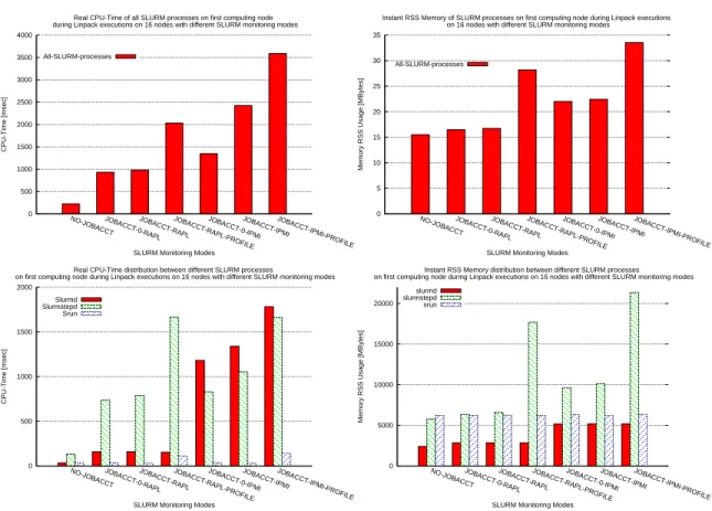
Fig. 2.CPU and Memory usage, tracked on first computing node, for all SLURM processes (top) and per different SLURM process

(bottom) for Linpack executions upon 16 computing nodes with different SLURM Montitoring Modes

Monitoring Modes Execution Time (s) Energy Consumption (J) Time Overhead Percentage Energy Overhead Percentage

NO JOBACCT 2657 12623276.73 -

-JOBACCT 0 RAPL 2658 12634455.87 0.04% 0.09%

JOBACCT RAPL 2658 12645455.87 0.04% 0.18%

JOBACCT RAPL PROFILE 2658 12656320.47 0.04% 0.26%

JOBACCT 0 IPMI 2658 12649197.41 0.04% 0.2%

JOBACCT IPMI 2659 12674820.52 0.07% 0.41%

JOBACCT IPMI PROFILE 2661 12692382.01 0.15 % 0.54%

Table 1.Monitoring Modes Comparisons in terms of Execution Times and Energy Consumption for Linpack deployment upon 16

nodes

The configuration of the Linpack executions was made in order to take about 80% of the memory per node and it take about 44 minutes to execute upon this platform which is a sufficient time to see how the different SLURM processes

(9)

may influence its execution. We have launched different executions for each monitoring mode and figure 2 presents our observations concerning CPU and Memory usage on the first computing node of the computation. We have performed 5 repetitions for each monitoring mode and the results presented on figure 2 had less than 1% differences.

At first sight we see that each monitoring mode involves different overheads. As expected the IPMI modes have bigger overheads than the RAPL ones. The worst case overhead is 3.5 sec for CPU-Time and 34MB for RSS in the case of IPMI plugin with profiling. We have tracked the CPU and Memory usage of the MPI processes as well but due to the big difference with SLURM processes in the order of magnitudes (around 30K sec for CPU time and 27GB for RSS) we do not display them on the same graphics. There is indeed an important difference in overhead with monitoring disabled and the various monitoring modes but if we compare it with the actual MPI CPU-Time even the worst case of 3.5 sec and 34MB of RSS seems benign.

It is interesting to see how the CPU-Time and Memory usage is distributed between the different SLURM processes. The bottom graphics in figure 2 confirm our expectations during the design of the features as described in section 3. As far as the CPU overhead concern we observe that slurmstepd usage increases significantly when monitoring is activated no matter if it is RAPL or IPMI. This is because of the polling thread launched from slurmstepd on job submission which is responsible for monitoring the various resources. We can also see how slurmstepd usage increases more when profiling is activated. This is due to the new thread which is launched within slurmstepd and that is responsible for the logging of energy consumption data on the hdf5 files. There is an important difference between the slurmd CPU usage when having IPMI instead of RAPL plugin activated. As explained in section 3, this is due to the fact that, for the IPMI plugin, a thread is launched within slurmd to poll data from the BMC asynchronously. It caches that information in order to avoid potential delays during further retrievals because of the freeipmi protocol overhead or the BMC itself. The CPU usage is also influenced by the sampling of energy polling and profiling. Lower frequency sampling would result in higher CPU-Time Usage. In our case we have set the sampling for the IPMI logic on the slurmd thread to 1 sec and the profling also to 1 sec which are the lowest values that can currently be configured. The communications between threads take place through RPC calls and since there are more info to exchange between the processes as we go towards more detailed monitoring, the slurmd usage increases gradually

Concerning the memory usage of slurmd, the new IPMI thread is responsible for the memory consumption increase. The significant increase in memory usage on the slurmstepd side when having profiling activated, is explained by the memory reserved for hdf5 internals. As a matter of fact, even if the RSS value for memory consumption remains stable during the execution, it is interesting to note that in the case of profiling, the RSS starts with a high value that gradually increases during the computation. The value ploted in the graphics is the maximum RSS usage which was observed just before the end of the job.

We have observed the actual overheads in terms of CPU and Memory upon each computing node during job execution. We then need to evaluate their effects on the actual computations. Our concern is not only that it uses the same resources as the actual execution, but that the interference of the slurm processes may destabilize the execution of each MPI process or influence their interactions. This would have effect in either the execution time or the energy consumption. Table 1 show the differences in terms of these characteristics. The results on table 1 do not actually describe the general case but rather a tendency. In particular the results in figure 2 are true on every repetitions but the results on table 1 represent the median of the 5 repetitions per monitoring mode. There were runs where the actual overhead changed slightly, modifying the order between the monitoring modes, but their overhead percentages never increased more than 0.2% for execution time and 0.6% for energy consumption. This detail further confirms that the execution and energy consumption are not influenced by the monitoring mode.

In this study we do not profile the Network usage to see if SLURM exchanges influences the MPI communications. One of the reasons is that in real production systems SLURM communications and applications communications go through different networks.

4.3 Measurements Precision Evaluation

SLURM has been extended to provide the overall energy consumption of an execution and to provide a mean to profile the instant power consumption per job on each node. The overall energy consumption of a particular job is added to the Slurm accounting DB as a new step characteristic. The instant power consumption of a job is profiled specifically on each node and logged upon hdf5 files. Each plugin, IPMI or RAPL, has these two different ways of logging energy and instant power.

In this section we evaluate the accuracy of both logging mechanisms for IPMI and RAPL plugins. The acquired mea-surements are compared to the meamea-surements reported from the Power-meters . As the power-meters report instant power consumptions per node, we can directly compare them with the acquired values for instant power. However, IPMI is the

(10)

only plugin that measures at the same level as the Power-meters, RAPL plugin only reporting at the level of sockets, thus limiting the comparisons to the sensibility and tendency of power consumptions and not the exact values.

The comparisons are presented through two different forms : either graphs to compare the instant power consumption per node or per job and tables to compare the overall energy consumption per job. The data used for the plotted graphics representing the instant power consumption evaluations are collected externally from the Watt-meters and from the hdf5 files that are constructed internally on each node by the SLURM monitoring mechanisms. The data used for the tables representing the energy consumption comparisons are produced from calculations of energy per job using the Watt-meter values and for the SLURM case they are retrieved by the SLURM accounting database after the end of the job.

In order to cover different job categories we conducted experiments with 3 different benchmarks for different durations and stressing of different kind of resources Hence the following benchmarks are used:

– long running jobs with Linpack benchmark which consumes mainly CPU and Memory and runs more then 40 minutes

for each case

– medium running jobs with IMB benchmark which stresses the network and runs about 15 minutes

– short running jobs with Stream benchmark which stresses mainly the memory and runs for about 2 minutes

0 500 1000 1500 2000 2500 100 150 200 250 300

Power consumption of one node measured through External Wattmeter and SLURM inband RAPL during a Linpack on 16 nodes

Time (sec) Instant P o w er Consumption [W att] 0 500 1000 1500 2000 2500 100 150 200 250 300 Time (sec) Type of collection − Calculated Energy Consumption

External Wattmeter − 749259.89 Joules SLURM inband RAPL − 518760 Joules

Power consumption of Linpack execution upon 16 nodes measured through External Wattmeter and SLURM inband RAPL

1000 1400 1800 2200 2600 3000 3400 3800 4200 4600 5000 5400 Consumption [W att] 0 500 1000 1500 2000 2500 Time [s]

Type of collection − Calculated Energy Consumption External Wattmeter − 12910841.44 Joules SLURM inband RAPL − 8458938 Joules

0 500 1000 1500 2000 2500

250

300

350

Power consumption of one node measured through External Wattmeter and SLURM inband IPMI during a Linpack on 16 nodes

Time (sec) Instant P o w er Consumption [W att] 0 500 1000 1500 2000 2500 250 300 350 Time (sec) Type of collection − Calculated Energy Consumption

External Wattmeter − 936237.93 Joules SLURM inband IPMI − 910812 Joules

Power consumption of Linpack execution upon 16 nodes measured through External Wattmeter and SLURM inband IPMI

4000 4200 4400 4600 4800 5000 Consumption [W att] 0 500 1000 1500 2000 2500 Time [s]

Type of collection − Calculated Energy Consumption External Wattmeter − 12611406.87 Joules SLURM inband IPMI − 12545568 Joules

Fig. 3.Precision for RAPL (top) and IPMI (bottom) with Linpack executions)

Long running jobs: The 2 top graphics of figure 3 show us results with executions of the Linpack benchmark and the

RAPL monitoring mode. The top left graphic refers to the instant power consumption of one node and the top right graphic shows the aggregated power consumption for all 16 nodes that participated in the computation. The red line represents measurements for the whole node (left) and all the whole nodes (right). The black line gives the power consumption of the 2 sockets and the associated memory banks of one node (left) and the aggregation of the same value for all the nodes (right). It is interesting to see how the RAPL graph follows exactly the Wattmeter graph which means that power consumption of the whole node is mainly defined by the CPU and memory plus a certain stable value which would reflect the other components of the system. Furthermore we realize that RAPL plugin is equally sensitive as a wattmeter in terms of power fluctuations.

These graphs show us that RAPL plugin with profiling activated can be used for energy profiling of the application with a very high sensitivity.

The 2 bottom graphics of figure 3 represent the comparison of Wattmeter and SLURM IPMI monitoring mode collections. We can see that IPMI values do not have the same sensitivity as Wattmeters or the one we can see with the RAPL plugins. Nevertheless, the black line of SLURM IPMI monitoring follows an average value along the fluctuations that

(11)

the Wattmeters may have. Hence in the end the final energy consumptions as calculated by producing the surfaces of the graphs have a fairly good precision that has less than 2% of error deviation.

Table 2 shows the precision of the internal algorithm used in SLURM IPMI monitoring mode to compute the overall energy consumption of the job. All computations use the Linpack benchmark based on the same configuration with only differences in the value of the CPU Frequency on all the computing nodes. It is interesting to see that the error deviation for those long running jobs is even less than 1% except for 2 cases where it increases up to 1.51%.

Monitoring Modes/ 2.301 2.3 2.2 2.1 2.0 1.9 1.8 1.7 1.6 1.5 1.4 1.3 1.2

CPU-Frequencies

External Wattmeter 12754247.9 12234773.92 12106046.58 12022993.23 12034150.98 12089444.89 12086545.51 12227059.66 12401076.21 12660924.25 12989792.06 13401105.05 13932355.15 Postreatment Value

SLURM IPMI 12708696 12251694 12116440 11994794 11998483 12187105 12093060 12136194 12518793 12512486 13107353 13197422 14015043 Reported Accounting Value

Error Deviation 0.35% 0.13% 0.08% 0.23% 0.29% 0.8% 0.05% 0.74% 0.94% 1.17% 0.89% 1.51% 0.58%

Table 2.SLURM IPMI precision in Accounting for Linpack executions

0 200 400 600 800 100 150 200 250 300

Power consumption of one node measured through External Wattmeter and SLURM inband RAPL during an IMB execution on 16 nodes

Time (sec) Instant P o w er Consumption [W att] 0 200 400 600 800 100 150 200 250 300 Time (sec) Type of collection − Calculated Energy Consumption

External Wattmeter − 273492.73 Joules SLURM inband RAPL − 144753 Joules

Power consumption of IMB execution upon 16 nodes measured through External Wattmeter and SLURM inband RAPL

1000 1200 1400 1600 1800 2000 2200 2400 2600 2800 3000 3200 3400 3600 3800 Instant P o w er Consumption [W att] 0 500 Time [s]

Type of collection − Total Calculated Energy Consumption External Wattmeter − 3551862.65 Joules SLURM inband RAPL − 2103582 Joules

0 200 400 600 800 1000 100 150 200 250 300

Power consumption of one node measured through External Wattmeter and SLURM inband IPMI during an IMB execution on 16 nodes

Time (sec) Instant P o w er Consumption [W att] 0 200 400 600 800 1000 100 150 200 250 300 Time (sec) Type of collection − Calculated Energy Consumption

Power consumption of IMB execution upon 16 nodes measured through External Wattmeter and SLURM inband IPMI

1600 1800 2000 2200 2400 2600 2800 3000 3200 3400 3600 3800 Instant P o w er Consumption [W att] 0 500 1000 Time [s]

Type of collection − Total Calculated Energy Consumption External Wattmeter − 3532714.96 Joules SLURM inband IPMI − 3448760 Joules

Fig. 4.Precision for RAPL (top) and IPMI (bottom) with IMB benchmark executions)

Medium running jobs: Figure 4 show the results observed with the execution of medium sized jobs (around 15min)

using the IMB benchmark. Similar to the previous figure, the graphics on top show comparisons of Wattmeter and RAPL while in the bottom we have Wattmeter with IPMI.

The RAPL plugin graphics show once more that those measurements follow closely the ones of Wattmeters. On the other hand, IPMI plugin shows some shifting to the right compared to the Wattmeters trace. The explanation of this delay is further discussed later on. We can see the black line following a slow fluctuation within average values of the Wattmeter values.

In terms of energy consumption calculation we can see that the error deviations remain on acceptable rates mainly lower than 2% except for 3 cases with error deviations higher than 1.7%. For jobs with a smaller duration, the IPMI plugin lost accuracy for both instant power and energy consumption calculation.

CPU-Frequencies

Error Deviation 0.77% 0.61% 0.01% 0.88% 0.05% 0.62% 1.01% 0.52% 1.77% 0.75% 0.35% 2.09% 1.75%

Table 3.SLURM IPMI precision in Accounting for IMB benchmark executions

Short running jobs: In figure 5 we present the measurements obtained with short sized jobs (no more than 2.5min

per execution) with Stream benchmark. Similarly with the previous figure the graphics on the top show comparisons of Wattmeter and RAPL while in the bottom we have Wattmeter with IPMI.

(12)

0 50 100 150

150

200

250

300

Power consumption of one node measured through External Wattmeter and SLURM inband RAPL during stream execution on 16 nodes

Time (sec) Instant P o w er Consumption [W att] 0 50 100 150 150 200 250 300 Time (sec) Type of collection − Calculated Energy Consumption

Power consumption of stream execution upon 16 nodes measured through External Wattmeter and SLURM inband IPMI

2200 2400 2600 2800 3000 3200 3400 3600 3800 4000 4200 Instant P o w er Consumption [W att] 0 50 100 150 Time [s] Type of collection − Total Calculated Energy Consumption

0 50 100 150

100

150

200

250

Power consumption of one node measured through External Wattmeter and SLURM inband IPMI during stream execution on 16 nodes

Time (sec) Instant P o w er Consumption [W att] 0 50 100 150 100 150 200 250 Time (sec)

Type of collection − Calculated Energy Consumption External Wattmeter − 37854.92 Joules SLURM inband IPMI − 33208 Joules

Power consumption of stream execution upon 16 nodes measured through External Wattmeter and SLURM inband IPMI

1400 1600 1800 2000 2200 2400 2600 2800 3000 3200 3400 3600 3800 4000 4200 Instant P o w er Consumption [W att] 0 50 100 150 Time [s]

Type of collection − Total Calculated Energy Consumption External Wattmeter − 627555.9 Joules SLURM inband IPMI − 541030 Joules

Fig. 5.Precision for RAPL (top) and IPMI (bottom) with stream benchmark executions)

The Stream benchmark is mainly a memory bound application and based on that we can deduce that the small fluctuations of the Watt-meters (red line) are produced by memory usage. The RAPL plugin graphics shows a smaller sensitivity in comparison with the Wattmeter and this is because the actual memory is not measured through RAPL. Nevertheless the RAPL model provides a reliable copy of what happens in reality and proves that even for small jobs it is interesting to use this plugin for profiling. IPMI plugin gives a different view where the shift we observed in the medium running jobs and didn’t even exist in long running jobs, is here relatively important. We see that the IPMI black line grows slowly during about 70 seconds until it reaches the reference value of the Watt-meters. In figure 5 the growth had nearly the same duration. We can also observe the same tendency in the right graph for all the nodes that participated in the computation. Similarly with instant power consumption the calculation of energy consumption presents an important error deviation between Wattmeter values and IPMI ones, that goes even beyond 10% (table 4). It is interesting to observe how the error deviation drops while we decrease the CPU Frequency. This is because higher frequencies tend to finish faster and lower frequencies induce longer execution times. This means that the increase duration of IPMI graph tends to be kept around the same values (70 sec) and this makes the surface which give the energy consumption to be closer to the reference one. That is why when we pass on another level of duration the error deviation drops even lower than 2% as we saw on tables 2 and 3 for the long and medium sized jobs. Actually, the 70 sec increase when using IPMI is related to a hardware phenomenon and takes place even on figure 3. However, due to the long execution time of more than 2600 sec in that case, we can not really see it on the graph as it is marginal.

CPU-Frequencies

Error Deviation 13.19% 12.49% 11.84% 12.22% 10.74% 11.45% 9.85% 9.79% 10.23% 8.61% 8.82% 8.67% 6.02 %

Table 4.SLURM IPMI precision in Accounting for stream executions

The differences noticed between the Watt-meters and the IPMI plugin seems to be mostly due to the shift made by the slowly responsive increase in power consumption at the initialization of the job. In order to explain that phenomenon, we made some additional evaluations. First, we used a manual polling using the freeipmi calls in order to check against an issue within the SLURM IPMI implementation. The shift remained the same, a good point for the implementation, a bad news for the the freeipmi logic or the BMC side. Our suspicion at that time was that there probably was a hardware pheonomenon related to the IPMI polling. Hence in order to check against that we made a SLURM setup on a different model of hardware (using a different BMC) and deployed a simple CPU stressing execution of a multi-threaded prime number computation. As we did not have wattmeters for reference figures in that machine but as RAPL was proved to follow closely the Wattmeter tendency, we took that latter as a reference instead. Figure 6 shows the execution of a simple CPU bound application with SLURM -IPMI and SLURM - RAPL plugins on two different machines: One with

(13)

0 20 40 60 80 100 80 100 120 140 160 180 200

Power consumption of one DELL node measured through SLURM inband IPMI or RAPL during prime number calculations program

Time (sec) Instant P o w er Consumption [W att] 0 20 40 60 80 100 80 100 120 140 160 180 200 Time (sec) Type of collection

SLURM inband IPMI SLURM inband RAPL

0 20 40 60 80 140 160 180 200 220 240

Power consumption of one BULL node measured through SLURM inband IPMI or RAPL during prime number calculations program

Time (sec) Instant P o w er Consumption [W att] 0 20 40 60 80 140 160 180 200 220 240 Time (sec) Type of collection

SLURM inband IPMI SLURM inband RAPL

Fig. 6.RAPL and IPMI precision upon different nodes with different versions of BMC

the DELL- Poweredge R720 that we used in all our previous experiments and one with a BULL B710 node. We can see that the delayed increase we observed on our previous experiments is confirmed one more time on the orignial machine with this application (left graph). However we observe that there is practically no delay at all on the other technology of machines (right graph). It is worthy to note that we do not see any improvement on the sensitivity of the actual values in comparison with the reference ones.

Hence we can deduce that the problematic increase and shift of measurements depends firmly on the BMC type and can change depending on the architecture or the firmware of the BMC. So the precision of the power consumption and energy consumption calculations depend on the actual hardware and while the technology gets better we expect that the precision of our measurements will be improved. Unfortunately we did not have tha ability to provide complete executions with newer machines hardware to see how exactly the error deviation is diminished, but initial observations on figure 6 show us promising results. Furthermore, since the overhead of the monitoring modes was low as seen in the previous section, future works may allow the usage of internal sampling frequency lower than 1 second which can further improve the precision of power and energy data.

4.4 Performance-Energy Trade-offs

In this section we are interested in the observation of performance-energy trade-offs with particular applications. This kind of tests is common for dedicated profiling programs like PAPI but the interesting part now is that a Resource and Job Management System such as SLURM has been extended to have the same capabilities configurable at run time. The tracking of performance and energy consumption can be made either during the execution with particular commands (sstat or scontrol show node) or at the end of the job with results directly stored in the SLURM database or on hdf5 files dedicated for profiling. Furthermore this tracking is not passing from the overhead of the integration of a dedicated profiling program but rather through a direct integration of sensor polling inside the core of SLURM code. Hence this section shows the type of research that can be possible using the extensions on SLURM for monitoring and control of energy consumption and how these features can be helpful in order to make the right choice of CPU Frequency for the best performance-energy trade-off. We make use of three different benchmarks (Linpack, IMB and stream) and make various runs by changing the CPU Frequency and compare the overall energy consumption of the whole job. For this we use the setting of CPU Frequency through the particular parameter of (cpufreq) on the job submission. Concerning the measurements we compare the IPMI and RAPL monitoring modes with the reference one using Wattmeters.

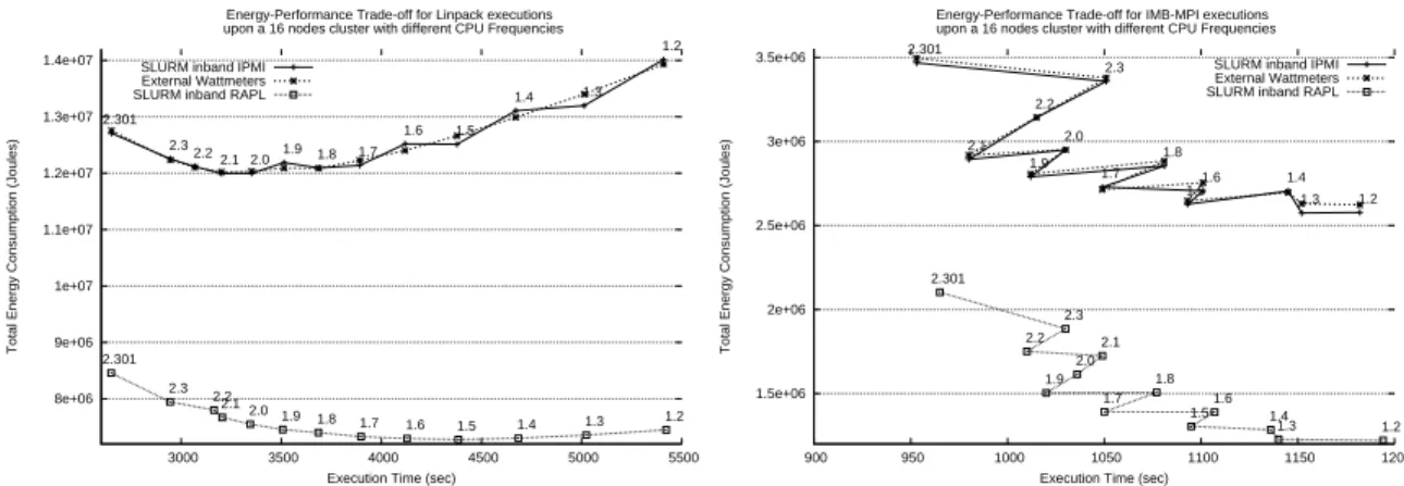
The figures that follow show the performance-energy tradeoffs with different CPU Frequencies. Figure 7 shows us the runs for Linpack (left graphic) and IMB benchmark (right) and figure 8 shows us the runs for Stream benchmark. Linpack benchmark shows that the turbo mode using a frequency of 2.301GHz gives the fastsest run but is fairly higher in terms of energy consumption. The lowest energy consumption is reached using 2.1GHz and in fact this is the best tradeoff between energy and performance. We can also observe that while the energy consumption is droping until this frequency it kind of stabilizes then with higher executions times until 1.7 GHz but increases after that. It is intersting to see that dropping the frequency lower than 1.4 has no benefit at all because we lose both in energy and performance in comparison with the turbo mode. Between IPMI and Wattmeter graphs there are some small differences but in general the IPMI follows closely the same tendencies of Wattmeters which proves that we can trust this kind of monitoring for this type of energy-performance profiling too. If we do not specify a particular frequency, Linux kernel decides which frequency the run will be made according to particular settings on the CPU scaling modules. The most common is the

(14)

on-demand where the run will be made on the higher frequency that exists. RAPL graph for the Linpack benchmark (left) shows us a kind of different behaviour with best tradeoff performance-energy between the frequencies 1.6 and 1.5. In addition we do not see the same tendency like the Wattmeter or IPMI graphs. This is related to the fact that RAPL only monitors a partial view of the active elements of the node, elements for which the energy consumption is mostly related to the frequency (and thus voltage) of the cores. The static consumption of the nodes, including the disks, network cards, motherboard chipsets and every others electrical components or fans are not took into account in RAPL. Increasing the computation time of an application involves increasing the share of the energy usage of all these second tier elements up to counter-balancing the benefits of running at a lower frequency. If the node was only made of sockets, RAPL shows that the best frequency to save energy would be lower than 1.5GHz.

8e+06 9e+06 1e+07 1.1e+07 1.2e+07 1.3e+07 1.4e+07 3000 3500 4000 4500 5000 5500

Total Energy Consumption (Joules)

Execution Time (sec) Energy-Performance Trade-off for Linpack executions upon a 16 nodes cluster with different CPU Frequencies SLURM inband IPMI

2.301 2.3_2.2 2.1 2.01.9 1.8 1.7 1.6 1.5 1.4 1.3 1.2 External Wattmeters

SLURM inband RAPL

2.301 2.3 2.2 2.1_2.0 1.9 1.8 1.7 1.6 1.5 1.4 1.3 1.2 1.5e+06 2e+06 2.5e+06 3e+06 3.5e+06 900 950 1000 1050 1100 1150 1200

Execution Time (sec) Energy-Performance Trade-off for IMB-MPI executions upon a 16 nodes cluster with different CPU Frequencies

SLURM inband IPMI 2.301 2.3 2.2 2.1 2.0 1.9 1.8 1.7 1.6 1.5 1.4 1.3 1.2 External Wattmeters SLURM inband RAPL

2.301 2.3 2.2 2.1 2.0 1.9 1.8 1.7 1.6 1.5 1.4 1.3 1.2

Fig. 7.Energy-Time Tradeoffs for Linpack (left) and IMB (right) benchmarks and different CPU frequencies

300000 350000 400000 450000 500000 550000 600000 650000 150 160 170 180 190 200

Execution Time (sec) Energy-Performance Trade-off for stream executions upon a 16 nodes cluster with different CPU Frequencies

External Wattmeters 2.301 2.3 2.2 2.1 2.0 1.9 1.8 1.7 1.6 1.5 1.4 1.3 1.2 SLURM inband IPMI

2.301 2.3 2.2 2.1 2.0 1.91.8 1.7_1.6 1.5 1.4 1.3 1.2 SLURM inband RAPL

2.301 2.3 2.2 2.1 2.0 1.9 1.8 1.7 1.6 1.5 1.4 1.3 1.2

Fig. 8.Energy Time tradeoffs for Stream benchmark and different CPU frequencies

IMB benchmark on the right has a different appearance than Linpack. For example frequency of 2.1 has better energy consumption and performance than 2.2 or 2.3 and then again 1.9 is better in both in comparison with 2.0. The best trade-off between energy and performance would probably be either 2.1 , 1.9 or 1.7. If we consider the RAPL graph 1.9 would be probably the best choice. IMB benchamark mainly stresses the Network and that is why small changes in CPU frequency have different kind of effects on performance and energy that is why the graph has nothing to do with linear or logarithmic evolution.

Finally on figure 8 we can see graphically the error deviation of IPMI vs Wattmeters that we observed on table 4. We can observe that the best tradeoff is performed with Frequencies 1.6 or 1.5 . It is interesting to see how this graph has an obvious logarithmic design with stability on execution times and changes on energy from 2.301GHz until 1.6 and stability on energy consumption and changes on execution times from 1.6 until 1.2. This makes it easier to find the best choice of CPU-Frequency for performance-energy tradeoffs. We can also observe how the difference of IPMI values with

(15)

Wattmeters which are due to the BMC delays as we have explained in the previous section tend to become smaller as the time of execution grows.

Overall, it is interesting to see how each application has different tradeoffs. That is the reason why particular profiling is needed for every application to find exactly the best way to execute it in terms of both energy and performance. The outcome of these evaluations is to raise the importance of energy profiling to improve the behaviour of the applications in terms of performance and energy and show how the new extensions in SLURM can be used to help the user for this task and find the best tradeoffs in energy and performance. Furthermore the comparison of monitoring modes with Wattmeters proves that SLURM internal monitoring modes provide a reliable way to monitor the overall energy consumption and that controlling the CPU Frequency is made correctly with real changes on performance and energy. We argue that most real life applications have execution times far bigger than our long running jobs here (Linpack) so the energy performance tradeoffs will definitely be more important than reported in this paper.

5 Conclusions and future works

This paper presents the architecture of a new energy accounting and control framework integrated upon SLURM Resource and Job Management System. The framework is composed of mechanisms to collect power and energy measurements from node level built-in interfaces such as IPMI and RAPL. The collected measurements can be used for job energy accounting by calculating the associated consumed energy and for application power profiling by logging power with timestamps in HDF5 files. Furthermore, it allows users to control the energy consumption by selecting the CPU Frequency used for their executions.

We evaluated the overhead of the framework by executing the Linpack benchmark and our study showed that the cost of using the framework is limited; less than 0.6% in energy consumption and less than 0.2% in execution time. In addition, we evaluated the precision of the collected measurements and the internal power-to-energy calculations and vice versa by comparing them to measures collected from integrated Wattmeters. Our experiments showed very good precision in the job’s energy calculation with IPMI and even if we observed a precision degradation with short jobs, newer BMC hardware showed significant improvements. Hence our study shows that the framework may be safely used in large scale clusters such as Curie and no power-meters are needed to add energy consumption in job accounting.

In terms of power profiling with timestamps, IPMI monitoring modes had poor sensitivity but the actual average values were correct. On the other hand, RAPL monitoring modes, which capture only sockets and DRAM related informations, had very good sensitivity in terms of power profiling but the energy consumption could not be compared with the energy calculation from the Wattmeters data. Indeed, the RAPL provides interesting insights about the processors and DRAM energy consumptions but does not represent the real amount of energy consumed by a node. It would thus be interesting to use both the IPMI and the RAPL logics at the same time in further studies. This would help to identify the evolution of the consumption of the other active parts of the node over time. Having a similar ability to monitor and control these active parts, like hard-disk drives and interconnect adapters, could help to go further in the description and the adaptation of the power consumption of the nodes according to applications needs. This particular field of interest is getting an increasing attention, as witnessed by the ISC’13 Gauss Award winner publication [22] concerning the interest of having the capability to differentiate the IT usage effectiveness of nodes to get more relevant energy indicators. Enhanced and fine-grained energy monitoring and stearing of more node components would really help to make an other step forward in energy efficient computations.

Treating energy as a new job characteristic opens new doors to treat is as a new resource. The next phase of this project will be to charge users for power consumption as a means of aligning the user’s interest with that of the organization providing the compute resources. In this sense, energy fairsharing should be implemented to keep the fairness of energy distribution amongst users. Any resource for which there is no charge will likely be treated by users as a resource of no value, which is clearly far from being the case when it comes to power consumption.

Longer term plans call for leveraging the infrastructure described in this paper to optimize computer throughput with respect to energy availability. Specifically the optimization of system throughput within a dynamic power cap reflecting the evolutions of the amount of available power over time seems necessary. It could help to make a larger use of less expensive energy at night for CPU intensive tasks while remaining at a lower threshold of energy consumption during global demand peaks, executing memory or network intensive applications.

Continuing research in the area of energy consumption is mandatory for the next decades. Having in mind the impact of the power consumption on the environment, even a major break in computation technology enabling more efficient execution would not change that fact. The HPC ecosystem needs to minimize its impact for long term sustainability and managing power efficiently is a key part in that direction.

(16)

6 Acknowledgements

The authors would like to thank Francis Belot from CEA-DAM for his advices on the energy accounting design and his comments on the article. Experiments presented in this paper were carried out using the Grid’5000 experimental testbed, being developed under the INRIA ALADDIN development action with support from CNRS, RENATER and several Universities as well as other funding bodies (see https://www.grid5000.fr).

References

1. Yoo, A.B., Jette, M.A., Grondona, M.: SLURM: Simple Linux utility for resource management. In Feitelson, D.G., Rudolph, L., Schwiegelshohn, U., eds.: Job Scheduling Strategies for Parallel Processing. Springer Verlag (2003) 44–60 Lect. Notes Comput. Sci. vol. 2862.

2. : Top500 supercomputer sites. (http://www.top500.org/)

3. Assunção, M., Gelas, J.P., Lefèvre, L., Orgerie, A.C.: The green grid’5000: Instrumenting and using a grid with energy sensors. In: Remote Instrumentation for eScience and Related Aspects. Springer New York (2012) 25–42

4. James, L., David, D., Phi, P.: Powerinsight - a commodity power measurement capability. The Third International Workshop on Power Measurement and Profiling (2013)

5. Ge, R., Feng, X., Song, S., Chang, H.C., Li, D., Cameron, K.: Powerpack: Energy profiling and analysis of high-performance systems and applications. Parallel and Distributed Systems, IEEE Transactions on 21(5) (2010) 658–671

6. Intel: (”intelligent platform management interface specification v2.0”)

7. Hackenberg, D., Ilsche, T., Schone, R., Molka, D., Schmidt, M., Nagel, W.E.: Power measurement techniques on standard com-pute nodes: A quantitative comparison. In: Performance Analysis of Systems and Software (ISPASS), 2013 IEEE International Symposium on. (2013) 194–204

8. Rotem, E., Naveh, A., Ananthakrishnan, A., Weissmann, E., Rajwan, D.: Power-management architecture of the intel microarchi-tecture code-named sandy bridge. IEEE Micro 32(2) (2012) 20–27

9. Dongarra, J., Ltaief, H., Luszczek, P., Weaver, V.: Energy footprint of advanced dense numerical linear algebra using tile algorithms on multicore architectures. In: Cloud and Green Computing (CGC), 2012 Second International Conference on. (2012) 274–281 10. Hähnel, M., Döbel, B., Völp, M., Härtig, H.: Measuring energy consumption for short code paths using rapl. SIGMETRICS

Perform. Eval. Rev. 40(3) (2012) 13–17

11. Weaver, V.M., Johnson, M., Kasichayanula, K., Ralph, J., Luszczek, P., Terpstra, D., Moore, S.: Measuring energy and power with papi. In: ICPP Workshops. (2012) 262–268

12. Goel, B., McKee, S., Gioiosa, R., Singh, K., Bhadauria, M., Cesati, M.: Portable, scalable, per-core power estimation for intelligent resource management. In: Green Computing Conference, 2010 International. (2010) 135–146

13. Eschweiler, D., Wagner, M., Geimer, M., Kn¨upfer, A., Nagel, W.E., Wolf, F.: Open trace format 2: The next generation of scalable trace formats and support libraries. In Bosschere, K.D., D’Hollander, E.H., Joubert, G.R., Padua, D.A., Peters, F.J., Sawyer, M., eds.: PARCO. Volume 22 of Advances in Parallel Computing., IOS Press (2011) 481–490

14. Folk, M., Cheng, A., Yates, K.: HDF5: A file format and i/o library for high performance computing applications. In: Proceedings of Supercomputing’99 (CD-ROM), Portland, OR, ACM SIGARCH and IEEE (1999)

15. Biddiscombe, J., Soumagne, J., Oger, G., Guibert, D., Piccinali, J.G.: Parallel computational steering for HPC applications using HDF5 files in distributed shared memory. IEEE Transactions on Visualization and Computer Graphics 18(6) (2012) 852–864 16. Hennecke, M., Frings, W., Homberg, W., Zitz, A., Knobloch, M., B¨ottiger, H.: Measuring power consumption on ibm blue gene/p.

Computer Science - Research and Development 27(4) (2012) 329–336

17. Rountree, B., Lownenthal, D.K., de Supinski, B.R., Schulz, M., Freeh, V.W., Bletsch, T.: Adagio: making dvs practical for complex hpc applications. In: ICS ’09: Proceedings of the 23rd international conference on Supercomputing, New York, NY, USA, ACM (2009) 460–469

18. Huang, S., Feng, W.: Energy-efficient cluster computing via accurate workload characterization. In: CCGRID ’09: Proceedings of the 2009 9th IEEE/ACM International Symposium on Cluster Computing and the Grid, Washington, DC, USA, IEEE Computer Society (2009) 68–75

19. Lim, M.Y., Freeh, V.W., Lowenthal, D.K.: Adaptive, transparent frequency and voltage scaling of communication phases in mpi programs. In: SC ’06: Proceedings of the 2006 ACM/IEEE conference on Supercomputing, New York, NY, USA, ACM (2006) 107

20. Costa, G.D., de Assunção, M.D., Gelas, J.P., Georgiou, Y., Lefèvre, L., Orgerie, A.C., Pierson, J.M., Richard, O., Sayah, A.: Multi-facet approach to reduce energy consumption in clouds and grids: the green-net framework. In: e-Energy. (2010) 95–104 21. Bolze, R., Cappello, F., Caron, E., Daydé, M., Desprez, F., Jeannot, E., Jégou, Y., Lantéri, S., Leduc, J., Melab, N., Mornet, G.,

Namyst, R., Primet, P., Quetier, B., Richard, O., Talbi, l.G., Ir´ea, T.: Grid’5000: a large scale and highly reconfigurable experimental grid testbed. Int. Journal of High Performance Computing Applications 20(4) (2006) 481–494

22. Patterson, M., Poole, S., Hsu, C.H., Maxwell, D., Tschudi, W., Coles, H., Martinez, D., Bates, N.: Tue, a new energy-efficiency metric applied at ornl’s jaguar. In Kunkel, J., Ludwig, T., Meuer, H., eds.: Supercomputing. Volume 7905 of Lecture Notes in Computer Science. Springer Berlin Heidelberg (2013) 372–382