Sudden change detection in turbofan engine behavior

HAL Id: hal-00662337

https://hal.archives-ouvertes.fr/hal-00662337

HAL is a multi-disciplinary open access archive for the deposit and dissemination of sci-entific research documents, whether they are pub-lished or not. The documents may come from teaching and research institutions in France or abroad, or from public or private research centers.

L’archive ouverte pluridisciplinaire HAL, est destinée au dépôt et à la diffusion de documents scientifiques de niveau recherche, publiés ou non, émanant des établissements d’enseignement et de recherche français ou étrangers, des laboratoires publics ou privés.

Sudden change detection in turbofan engine behavior

Jérôme Lacaille, Etienne Côme

To cite this version:

Jérôme Lacaille, Etienne Côme. Sudden change detection in turbofan engine behavior. Interna-tional Conference on Condition Monitoring and Machinery Failure Prevention Technologies, Jun 2011, Cardiff, United Kingdom. pp.542-548. �hal-00662337�

Sudden change detection in turbofan engine behavior

Jérôme Lacaille Snecma

Villaroche, 7550 Moissy-Cramayel cedex, France Tel. : +33 1 60 59 70 24

Fax : +33 1 60 59 89 22

jerome.lacaille@snecma.fr

Etienne Côme IFSTAR/INRETS

2 rue de la Butte Verte, 93166 Noisy le Grand cedex, France Tel. : +33 1 45 92 55 00

Fax : +33 1 45 92 55 01

etienne.comes@inrets.fr

Abstract

Turbofan engines generate a lot of data for maintenance purpose. During each flight the aircraft send information to the ground using small messages. On those messages one can find a description of the engine behavior (shaft speed, oil temperature, pressures, etc.) and the observation context (air temperature, aircraft attitude, altitude, etc.). Mainly those signals are used for trend analysis which goal is wear detection and scheduling for shop visits. But the temporal curves obtained this way also hide some very interesting fleeting events that may be connected to sudden changes in the turbofan configuration. The changes of our interest are buried in the signal noise and are often hidden by the flight context variation. To reveal those events one uses two successive original algorithms. The first one resolves the context dependency and the second filters the signal using change detection. The filtered signal with change information is compared to the flight log-book for validation purpose. One detects almost all known problems that were cause of maintenance operation but the algorithm also finds some unsuspected changes now under investigation…

1. Introduction

A civil aircraft send information to the ground: those small messages, at least two per flight at takeoff and cruise, are called ACARS for “Aircraft Communication Addressing and Reporting System”. They each weight at most 4Kb and contain measurements of the aircraft behaviour and its engines. The table below (Figure 1) shows some data that we collect on a fleet of 70 planes.

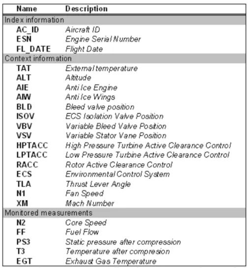
In this table one can identify three sections: data related to the plane, flight and engine numbers; context information that describes the behaviour of the plane during the data acquisition ; and some really engine-specific measurements.

Our interest is in the analysis of the multi-curve made of those 5 last measurements. The main question is: does that curve present some abnormality which may correspond to a real event that append in the engine life.

2

Figure 1: The measurements collected for one engine during a flight.

2. Methodology

The goal is to build clear and understandable multivariate trajectories for the engine states. The first step will remove all context dependent information from the observed five measurements. The first idea is to use a linear regression model. For each engine variable r=1...5 one would write

r ij q ij r ij r r r r ij X X Y q i λ λ ε α µ + + + + + = 1 L 1 ... (1)

Where i is the engine number and j is an observation. Each variable X is one analytic combination of context data, µ is the intercept for output variable r, α is the engine dependency on output variable r (one way to take the engine age into account) and ε is the residual vector.

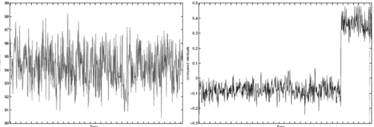
Figure 2 presents the rough measurements of the corespeed feature as a function of time (for engine #6) and the residuals computed by model (eq. 1). The rough measurements (on the left) seem almost time-independent on this figure, whereas the residuals exhibit an abrupt change which is linked to a specific event in the life of this engine. This simple model is therefore sufficient to bring to light interesting aspects of the evolution

of this engine. However, the signals may contain ruptures, making the use of a single regression model hazardous. This first algorithms, which is called ECN (for Environemental Condition Normalisation), uses a selection algorithms detailed in the next section to choose among a wide variety of different context-dependent input variables X.

Figure 2: The left side of this figure shows the initial corespeed (N2) of a given engine as measured by our sensors. The right side shows the residual of the same

measurement after regression on context data.

Once normalisation applied an on-line detection algorithm to find abrupt changes is used. This is a piecewise regression model. The detection of the change points is done with a multi-dimensional statistic test taking all the normalized engine variables supplied by ECN as input. The outputs of this second step called CD (for Change Detection) are the sudden change dates and the smoothed observations. These last data are finally used in a classification algorithm (a self organizing map) which was discussed in IEEE Aerospace Conference(20). This classification presents all engine state trajectories onto a 2D map and helps the engineers to identify trends in the engine behaviour. Given a well chosen distance between trajectory parts, it is possible to find similar (past) trajectories followed by older engines, and then being able to make statistical assumptions for the evolution of any current engine.

2. Environmental Conditions Normalization

The external context measurements are combined to build a set of predictors Xp,

p=1...q. Such combitations involves automatic computations of polynomes to the fourth

degree (squares, cubes, etc. and all corresponding cross-products) but also non-linear transforms (logarithms, exponentials, inverse) used in conjunction with expert knowledge to select only relevant computations (in adequation with the engine physical model). The number q of such input variables is really huge, moreover, most of the inital measurements are statistically linked together. Hence it is really important to select only the minimal amount of input variables to ensure a correct robustness of the linerar regression.

A LASSO criterion(3) is therefore used to estimate the regression parameters and to select a subset of significant predictors. This criterion can be written using the notations from chapter 2 for one engine variable Yr, r=1...5 as :

4

∑

∑

∑

The regression coefficients λp are penalized by a condition (L1 norm) which forces

some of them to be null for a well chosen value of C. The LARS algorithm(3) is used to estimate all the solutions of the LASSO criterion (eq. 2) for all possible values of C. The optimal value of C with respect to the prediction error estimated by cross-validation (with 20 folds) is finally selected. Engine variables are well explained by the proposed models as attested by the high value of the coefficients of determination.

Figure 3 : Number of predictors that where selected by the LARS/LASSO

algorithm and the computed coefficients of determination R2.

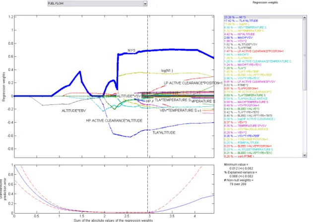
Figure 4: The result of the LARS/LASSO algorithm when selecting inputs for fuel

flow regression. The upper graph shows the coefficients λwhen the energy

constraint C increases. The lower graph gives the generalization error obtained by cross-validation. The selected solution is marked by a vertical dashed line. On the

A qualitative inspection of the model results was also carried out with the help of engine experts. The regularization path plot (as shown in Figure 4) is very interesting from the point of view of the experts, because it can be compared with their previous knowledge. Such a curve clearly highlights which are the more relevant predictors and they appear to be in good adequateness with the physical knowledge on the system.

3. Change Detection

To take into account the two types of variation (linear trend and abrupt changes), we implement an algorithm based on the ideas from Gustafsson(2) and Ross & all(4). The solution is based on the joint use of an on-line change detection algorithm to detect abrupt changes and of a bank of recursive least squares (RLS) algorithms to estimate the slow variations of the signals. The algorithm works on-line in order to allows projecting new measurements on the map as soon as new data are available.

The trend estimation use a recursive least squares algorithm. After initialization flight lm

the trend is estimated until current flight l (eq. 3). The model error is computed and tested according to chosen parameters.

(

)

∑

The parameter θ is a forgetting factor and the results αland βlare the intercept and the

slope computed for flight l. One computes the residual error vector [ 1, , 5]

l l

l ε ε

ε = K as

the difference, for each variable of the observed value and the estimated value using the current slope model. This vector is supposed to follow a Gaussian law.

) , ( Σ = l l N m ε ... (4) Where ml is the mean observed error and Σthe covariance matrix of residuals between

each measurements. The generalized likelihood ratio test should validate ||ml||<r0 for l<lm+1 and ||ml||>r1 for l>=lm+1 to detect a change at flight lm+1 (r0 and r1 are chosen

thresholds).

If the test detects a change at flight lm+1 the computation is reinitialized. This test is

implemented as a multivariate computation, thus when a change is detected all computations, on each variable, are reinitialized simultaneously. Figure 5 presents a sudden change well observed in temperatures and fuel flow. It is important that this whole process remains iterative, so the new smoothed observations are automatically computed and may be immediately treated by the classification algorithm.

6

Figure 5: Sudden changes were detected for this engine on exhaust gaz temperature and fuel flow.

4. Conclusions

This change detection algorithm was systematically applied on 140 engines that were followed during a little more than one year during which 120 maintenance operations occured. 92 changes were detected.

• 40% of the detected changes appear at most one month before a maintenance operation.

• 20% changes are less that one month after a maintenance operation. The other changes are unexplained and should eventually be investigated.

After this change detection, the residual signals are classified using a self organizing map (SOM) and the result is a 2D trajectory for each engine. The map on which those trajectories ar plotted shows some well identified clusters that will provide a good help for engineers to analyse the unexplained detections.

References

1. Basseville, M., Nikiforov, I.: Detection of Abrupt Changes: Theory and Application. Prentice-Hall (1993).

2. Gustafsson, F.: Adaptive filtering and change detection. John Wiley & Sons (2000).

3. Efron, B., Hastie, T., Johnstone, I., Tibshirani, R.J.: Least angle regression. Annals of Statistics 32(2), 407–499 (2004).

4. Ross, G., Tasoulis, D., Adams, N.: Online annotation and prediction for regime switching data streams. In: Proceedings of ACM Symposium on Applied Computing. pp. 1501–1505 (March 2009).

5. J. Lacaille, “Standardized Failure Signature for a Turbofan Engine”, in Proceedings of IEEE Aerospace Conference 2009, Big Sky, MO.

6. X. Flandrois, J. Lacaille, et all. “Expertise Transfer and Automatic Failure Classification for the Engine Start Capability System”, in Proceedings of AIAA Infotech 2009, Seattle, WA.

7. J. Lacaille, R. N. Djiki, “Model Based Actuator Control Loop Fault Detection”, in Proceedings of Euroturbo Conference 2009, Graz, Austria.

8. S. Blanchard et all. « Health Monitoring des moteurs d’avions », les entretiens de Toulouse 2009, France.

9. M. Cottrell et all. “Fault prediction in aircraft engines using Self-Organizing Maps”, in Proceedings of WSOM 2009, Miami, FL.

10. A. Ausloos et all. “Estimation of monitoring indicators using regression methods; Application to turbofan start sequence”, ESREL 2009, Prague, Poland.

11. J. Lacaille, “An Automatic Sensor Fault Detection and Correction Algorithm”, AIAA ATIO 2009, Hilton Beach, SC.

12. J. Lacaille, “A Maturation Environment to Develop and Manage Health Monitoring Algorithms”, PHM 2009, San Diego, CA.

13. R. Klein, “Model Based Approach for Identification of Gears and Bearings Failure Modes”, PHM 2009, San Diego, CA.

14. J. Lacaille. “Validation of Health Monitoring Algorithms for Civil Aircraft Engines”. In IEEE Aerospace Conference, Big Sky, MT, 2010.

15. E. Côme, M. Cottrell, M. Verleysen, and J. Lacaille. “Self Organizing Star (SOS) for Health Monitoring”. In ESANN, Bruges, 2010.

16. E. Côme, M. Cottrell, M. Verleysen, and J. Lacaille. “Aircraft Engine Health Monitoring using Self-Organizing Maps”. In ICDM, Berlin, Germany, 2010. 17. A. Hazan, M. Verleysen, M. Cottrell, and J. Lacaille. “Trajectory Clustering

for Vibration Detection in Aircraft Engines”. In ICDM, Berlin, Germany, 2010.

18. H. Hazan, M. Verleysen, M. Cottrell, J. Lacaille, “Linear smoothing of FRF for aircraft engine vibration monitoring”, ISMA 2010, Louvain.

19. J. Lacaille, V. Gerez, R. Zouari, “An Adaptive Anomaly Detector used in Turbofan Test Cells”, PHM 2010, Portland, OR.

20. J. Lacaille, E. Côme, “Visual Mining and Statistics for a Turbofan Engine Fleet”, in Proceedings of IEEE Aerospace Conference 2011, Big Sky, MT.