HAL Id: hal-01206677
https://hal.sorbonne-universite.fr/hal-01206677
Submitted on 29 Sep 2015
HAL is a multi-disciplinary open access
archive for the deposit and dissemination of
sci-entific research documents, whether they are
pub-lished or not. The documents may come from
teaching and research institutions in France or
abroad, or from public or private research centers.
L’archive ouverte pluridisciplinaire HAL, est
destinée au dépôt et à la diffusion de documents
scientifiques de niveau recherche, publiés ou non,
émanant des établissements d’enseignement et de
recherche français ou étrangers, des laboratoires
publics ou privés.
atmosphere
R. Wang, Yves Balkanski, O. Boucher, L. Bopp, A. Chappell, P. Ciais, D.
Hauglustaine, J. Peñuelas, S. Tao
To cite this version:
R. Wang, Yves Balkanski, O. Boucher, L. Bopp, A. Chappell, et al.. Sources, transport and deposition
of iron in the global atmosphere. Atmospheric Chemistry and Physics, European Geosciences Union,
2015, 15 (11), pp.6247-6270. �10.5194/acp-15-6247-2015�. �hal-01206677�
www.atmos-chem-phys.net/15/6247/2015/ doi:10.5194/acp-15-6247-2015
© Author(s) 2015. CC Attribution 3.0 License.
Sources, transport and deposition of iron in the global atmosphere
R. Wang1,2,3, Y. Balkanski1,3, O. Boucher4, L. Bopp1, A. Chappell5, P. Ciais1,3, D. Hauglustaine1, J. Peñuelas6,7, and S. Tao2,3
1Laboratoire des Sciences du Climat et de l’Environnement, CEA CNRS UVSQ, Gif-sur-Yvette, France
2Laboratory for Earth Surface Processes, College of Urban and Environmental Sciences, Peking University, Beijing, China
3Sino-French Institute for Earth System Science, College of Urban and Environmental Sciences, Peking University,
Beijing, China
4Laboratoire de Météorologie Dynamique, IPSL/CNRS, Université Pierre et Marie Curie, Paris, France
5CSIRO Land & Water National Research Flagship, G.P.O. Box 1666, Canberra, ACT 2601, Australia
6CSIC, Global Ecology Unit CREAF-CEAB-UAB, Cerdanyola del Vallès, 08193 Catalonia, Spain
7CREAF, Cerdanyola del Vallès, 08193 Catalonia, Spain
Correspondence to: R. Wang (rong.wang@lsce.ipsl.fr)
Received: 30 December 2014 – Published in Atmos. Chem. Phys. Discuss.: 12 March 2015 Revised: 11 May 2015 – Accepted: 13 May 2015 – Published: 8 June 2015
Abstract. Atmospheric deposition of iron (Fe) plays an important role in controlling oceanic primary productivity. However, the sources of Fe in the atmosphere are not well understood. In particular, the combustion sources of Fe and the subsequent deposition to the oceans have been accounted for in only few ocean biogeochemical models of the car-bon cycle. Here we used a mass-balance method to esti-mate the emissions of Fe from the combustion of fossil fuels and biomass by accounting for the Fe contents in fuel and the partitioning of Fe during combustion. The emissions of Fe attached to aerosols from combustion sources were esti-mated by particle size, and their uncertainties were quanti-fied by a Monte Carlo simulation. The emissions of Fe from mineral sources were estimated using the latest soil miner-alogical database to date. As a result, the total Fe emissions from combustion averaged for 1960–2007 were estimated to
be 5.3 Tg yr−1 (90 % confidence of 2.3 to 12.1). Of these
emissions, 1, 27 and 72 % were emitted in particles < 1 µm (PM1), 1–10 µm (PM1−10), and > 10 µm (PM>10), respec-tively, compared to a total Fe emission from mineral dust of
41.0 Tg yr−1 in a log-normal distribution with a mass
me-dian diameter of 2.5 µm and a geometric standard deviation of 2. For combustion sources, different temporal trends were found in fine and medium-to-coarse particles, with a notable
increase in Fe emissions in PM1 since 2000 due to an
in-crease in Fe emission from motor vehicles (from 0.008 to
0.0103 Tg yr−1in 2000 and 2007, respectively). These
emis-sions have been introduced in a global 3-D transport model
run at a spatial resolution of 0.94◦latitude by 1.28◦
longi-tude to evaluate our estimation of Fe emissions. The mod-elled Fe concentrations as monthly means were compared with the monthly (57 sites) or daily (768 sites) measured concentrations at a total of 825 sampling stations. The de-viation between modelled and observed Fe concentrations attached to aerosols at the surface was within a factor of 2 at most sampling stations, and the deviation was within a factor of 1.5 at sampling stations dominated by combustion sources. We analysed the relative contribution of combustion sources to total Fe concentrations over different regions of the world. The new mineralogical database led to a modest improvement in the simulation relative to station data even in dust-dominated regions, but could provide useful informa-tion on the chemical forms of Fe in dust for coupling with ocean biota models. We estimated a total Fe deposition sink
of 8.4 Tg yr−1over global oceans, 7 % of which originated
from the combustion sources. Our central estimates of Fe emissions from fossil fuel combustion (mainly from coal) are generally higher than those in previous studies, although they are within the uncertainty range of our estimates. In partic-ular, the higher than previously estimated Fe emission from coal combustion implies a larger atmospheric anthropogenic input of soluble Fe to the northern Atlantic and northern Pa-cific Oceans, which is expected to enhance the biological car-bon pump in those regions.
1 Introduction
Sea-water dissolved iron (Fe) concentration is a primary fac-tor that limits or co-limits the growth of phytoplankton in large regions of the global oceans (Martin et al., 1991; Moore et al., 2013). As such, Fe availability influences the trans-fer and sequestration of carbon into the deep ocean (Boyd et al., 2000; Moore et al., 2004). Both ice-core and marine-sediment records indicate high rates of aeolian dust and hence Fe supply to the oceans at the Last Glacial Maximum, implying a potential link between Fe availability, marine
pro-ductivity, atmospheric CO2and climate through Fe
fertiliza-tion (Martin, 1990; Ridgwell and Watson, 2002). Over the Industrial Era, the increase of Fe deposition in dust was
es-timated to be responsible for a decrease of atmospheric CO2
by 4 ppm (Mahowald et al., 2011), with a large uncertainty. Atmospheric deposition provides an important source of Fe to the marine biota (Martin, 1990; Duce and Tindale, 1991; Johnson et al., 1997; Fung et al., 2000; Gao et al., 2001; Conway and John, 2014). Early studies of the ef-fects of Fe fertilization, however, mostly focused on aeolian dust sources (Hand et al., 2004; Luo et al., 2003; Gregg et al., 2003; Moore et al., 2004; Mahowald et al., 2005; Fan et al., 2006). Observed concentrations of soluble Fe were not properly captured by the models simulating the atmo-spheric transport, chemical processing and deposition of Fe in aerosols (Hand et al., 2004; Luo et al., 2005; Fan et al., 2006), thus suggesting the existence of other sources. Guieu et al. (2005) proposed that the burning of biomass could be an additional source of soluble Fe in the Ligurian Sea. Chuang et al. (2005) reported that soluble Fe observed at an atmo-spheric deposition measurement station in Korea was not dominated by mineral sources, even during dust storms. Sed-wick et al. (2007) hypothesized that the anthropogenic emis-sions of Fe from combustion could play a significant role in the atmospheric input of bioavailable Fe to the surface of the Atlantic Ocean. However, few global models have accounted for the impact of Fe from combustion on the open-ocean bio-geochemistry (Krishnamurthy et al., 2009; Okin et al., 2011), due to large uncertainties for the sources and chemical forms of Fe from combustion.
The first estimate of Fe emissions from fossil fuels and
biomass burning reported a total Fe emission of 1.7 Tg yr−1
(Luo et al., 2008). Ito and Feng (2010) subsequently obtained
a lower estimate of 1.2 Tg yr−1. By applying a high emission
factor of Fe from ships and accounting for a large Fe solubil-ity from oil fly ash, Ito (2013) later derived the same total Fe
emission of 1.2 Tg yr−1, but with a significant contribution
by shipping to soluble Fe deposition over the northern Pa-cific Ocean and the East China Sea. These authors suggested that more work was required to reduce the uncertainty in Fe emissions, particularly from the combustion of petroleum and biomass.
The mineral composition of dust is a key factor in the chemical forms of Fe, and it determines the solubility and
thus the bioavailability of Fe. Nickovic et al. (2012) devel-oped a global data set to represent the mineral composition of soil in arid and semi-arid areas. This mineralogical data set improved the agreement between simulated and measured concentrations of soluble Fe (Nickovic et al., 2013; Ito and Xu, 2014). More recently, Journet et al. (2014) developed a new data set of soil mineralogy (including soil Fe content) covering most dust source regions of the world at a resolu-tion of 0.5◦×0.5◦, with the aim to improve the modelling of the chemical forms of Fe in dust.
In this study, we estimated the emissions of Fe from com-bustion sources for 222 countries/territories over the 1960 to 2007 period using a new method based on Fe content of fuel and Fe budget during combustion. We re-estimated Fe emis-sions from mineral sources based on the latest mineralogical database. Our estimates of Fe sources were evaluated by an atmospheric transport model at a fine resolution. The impact of the estimated combustion-related and mineral emissions of Fe on the model–data misfits at 825 stations measuring Fe concentration in surface aerosol and 30 stations measur-ing Fe deposition was investigated for different regions and stations.
2 Data and methodology
2.1 Emissions of Fe from combustion sources
A global emission inventory of Fe from combustion was de-veloped, covering 222 countries/territories and the 1960 to 2007 period. The sources of Fe emission included the com-bustion of coal, petroleum, biofuel and biomass (55 combus-tion fuel types, defined in Wang et al., 2013). In contrast to previous studies (Luo et al., 2008; Ito, 2013), the emission of Fe was calculated based on the Fe content in each type of fuel, the partitioning of Fe between residue ash, cyclone ash and fly ash, the size distribution of Fe-contained particles, and the efficiency of removal by different types of control de-vice. A similar method has been recently applied to estimate the emissions of phosphorus from combustion sources (Wang et al., 2015). Only the fly ash is emitted to the atmosphere but other types of ashes are not. For a specific combustion fuel type, the emission (E) can be calculated as
E = a · b · c · (1 − f ) ·X x=1 Jx· " 4 X y=1 Ay·(1 − Rx,y) # , (1)
where x is a given particle size discretized into n bins (two bins for petroleum and three bins for coal and biomass), y is a specific control device (cyclone, scrubber, electrostatic precipitator, or no control), a is the consumption of fuel, b is the completeness of combustion (defined as the fraction of fuel burnt in the fires), c is the Fe content of the fuel, f is the fraction of Fe retained in residue ash relative to the amount of Fe in burnt fuel, Jxis the fraction of Fe emitted in particle
size x, the Ayis the fraction of a specific control device, and
Rx,yis the removal efficiency of control device y for particle size x. For all parameters in Eq. (1), the values or ranges are listed in Table 1 and briefly described below. The Fe in coal
fly ash was divided into three size bins: 0.1–0.3 % in PM1
(diameter < 1 µm), 10–30 % in PM1−10 (diameter 1–10 µm),
and the remainder in PM>10 (diameter > 10 µm) (Querol et al., 1995; Yi et al., 2008). The Fe in biomass fly ash was
also divided into three size bins: 1–3 % in PM1, 50–60 % in
PM1−10, and the remainder in PM>10(Latva-Somppi et al.,
1998; Valmari et al., 1999). The Fe in oil fly ash was divided
into two size bins: 80–95 % in PM1 and the remainder in
PM1−10 (Mamane et al., 1986; Kittelson et al., 1998). Fuel
consumption data are distributed spatially at a 0.1◦×0.1◦
resolution in PKU-FUEL-2007 (Wang et al., 2013), estab-lished for year 2007, combined with country data to obtain temporal changes from 1960 to 2006 (Chen et al., 2014; Wang et al., 2014a). Fixed completeness of combustion (b) values were assigned to coal (98 %), petroleum (98 %), wood in stoves (88 %), wood in fireplaces (79 %) and crop residues (92 %) (Johnson et al., 2008; Lee et al., 2005; Zhang, et al., 2008). As the fuel consumptions for biomass burning have already accounted for the completeness of combustion based on the type of fires (van der Werf et al., 2010), we applied a combustion completeness of 100 % for them. The percentage
of each control device (Ay)was calculated by year and
coun-try in our previous studies (Chen et al., 2014; Wang et al., 2014a, b) using a method based on S-shaped curves (Grubler et al., 1999; Bond et al., 2007).
2.2 Fe content in fuel
Fe content in coal was derived for 45 major coal-producing countries, such as China, US, Russia, India, Indonesia and Australia, from the World Coal Quality Inventory (Tewalt et al., 2010), which is based upon 1379 measured data in each country. The collected Fe content in coal followed log-normal distributions (Supplement Fig. S1), and the means
and standard deviations (σ ) of log10-transformed Fe content
in coal were derived for each country (Table S1). Fe content of coal burned in each country was then calculated including imported coal using the coal-trading matrix among countries (Chen et al., 2014). The variation of Fe content among dif-ferent coal types (which differs by 20 % between bituminous coal and lignite produced in Turkey as an example) is smaller than that of coal produced in different countries and is thus ignored in our study. In addition to coal, Fe contents of wood, grass, and crop residues were taken from a review study (Vas-silev et al., 2010), also following log-normal distributions
(Fig. S1). The means and σ of the log10-transformed Fe
con-tents were thereby derived for wood, grass, and crop residues separately. We applied the Fe content in grass (−3.57 ± 0.34
for log10-transformed Fe content) for the savanna and
grass-land fires and the Fe content in wood (−3.45 ± 0.57) for the deforestation, forest, woodland and peat fires. In
addi-tion, the means and σ of Fe contents were 0.13 ± 0.09 % for dung cakes (Sager et al., 2007) and 0.00024 ± 0.00023 % for biodiesel (Chaves et al., 2011), 32 ± 2 ppm for fuel oil (Bet-tinelli et al., 1995), 13 ± 7 ppm for diesel, 3.3 ± 2.6 ppm for gasoline and 4.9 ± 3.3 ppm for liquefied petroleum gas (Kim et al., 2013).
2.3 Partitioning of Fe in combustion
The fraction of Fe retained in residue ash (f in Eq. 1) dur-ing coal combustion has been measured for few real-world facilities: 43–45 % in a power plant in India (Reddy et al., 2005), 30 % in a power plant equipped with a bag-house in China (Yi et al., 2008), 40 % in a fluidized bed boiler (Font et al., 2012), and 30–40 % (measured for Mn, which is sim-ilar to Fe) in two power plants in China (Tang et al., 2013). We therefore applied a percentage of 30–45 % for Fe retained in residue ash during the combustion of coal in industry and power plants. For the combustion of petroleum, 43 and 58 % of the Fe in petroleum in a small-fire-tube boiler and a com-bustor representative for a larger utility boiler, respectively, were emitted in fly ash (Linak and Miller, 2000). A range of 43–58 % was thus adopted for Fe emitted into fly ash for petroleum burned in power plants and industry. For solid bio-fuels burned in industry, 60–70 % of the Fe was retained in the residue ash (Ingerslev et al., 2011; Narodoslawsky et al., 1996), which was the range adopted in this study.
The budget of Fe from the combustion of petroleum by motor vehicles has received little attention, likely due to the low Fe content in petroleum. Wang et al. (2003) reported that 93 % Fe in petroleum was released into the atmosphere, and thus we applied a percentage of 93 ± 5 % for Fe emitted into the atmosphere.
The partitioning of Fe from the combustion of various fu-els in the residential sector has not been studied. The con-centrations of Fe in residue ash and fly ash are similar (Meij, 1994), so the fraction of Fe emitted into the atmosphere was derived from the ratio of the mass of Fe in fly ash to that in the fuel. We thereby derived the fraction of Fe retained in residue ash (f in Eq. 1) from the burning of anthracite coal (99.6 ± 0.4%) (Chen et al., 2006; Shen et al., 2010), bituminous coal (94 ± 3%) (Chen et al., 2006; Shen et al., 2010), crop residues (87 ± 8%) (Li et al., 2007), and wood (94 ± 5%) (Shen et al., 2012) burned in residential stoves or fireplaces.
Many studies measured the budget of elements other than Fe in the open burning of biomass. We collected the budget measured for elements whose physical and chemical prop-erties are similar to those for Fe (e.g. low volatility). In the literature, the percentage of the element transfer to the at-mosphere based on the element present in initial fuels was converted to that based on that in burnt fuels using the com-pleteness of combustion (Raison et al., 1985; Pivello and Coutinho, 1992; Mackensen et al., 1996; Holscher et al., 1997). Raison et al. (1985) reported that 44–59 % of the
Table 1. Parameters used in the estimation of Fe emissions from combustion sources.
Parameter Description Values or data sources
a Fuel consumption The fuel data was taken from a global 0.1◦×0.1◦fuel data set which is used
to construct a global CO2emission inventory
(Wang et al., 2013; available at http://inventory.pku.edu.cn/home.html).
b Completeness of combustion – coal (98 %);
– petroleum (98 %); – wood in stoves (88 %); – wood in fireplaces (79 %); – crop residues (92 %);
– biomass burning (considered in van der Werf et al., 2010).
c Fe content of the fuel – coal: based on Fe contents in coal produced by country (Table S2) and an
international coal-trading matrix Chen et al. (2014); – wood (a geometric mean of 0.036 % and range in Fig. S1); – crop residues (a geometric mean of 0.060 % and range in Fig. S1); – grass (a geometric mean of 0.027 % and range in Fig. S1); – dung cakes (0.13 ± 0.09 %);
– biodiesel (0.00024 ± 0.00023 %); – heavy fuel oil (32 ± 2 ppm); – diesel (13 ± 7 ppm); – gasoline (3.3 ± 2.6 ppm);
– liquefied petroleum gas (4.9 ± 3.3 ppm). f Fraction of Fe retained in residue ash relative – coal used in industry and power plants (30–45 %);
to the amount of Fe in the burnt fuel – petroleum used in industry and power plants (43–58 %); – solid biofuels used in industry and power plants (60–70 %); – petroleum consumed by motor vehicles (2–12 %); – anthracite coal used in the residential sector (99.2–99.8 %); – bituminous coal used in the residential sector (91–97 %); – crop residues used in the residential sector (79–95 %); – wood used in the residential sector (89–99 %); – forest fires (49–98 %);
– savanna fires (24–79 %); – deforestation (43–50 %);
– woodland fires/peat fires (41–56 %).
Jx Fraction of Fe emitted in a particle size – coal fly ash (0.1–0.3 % in PM1; 10–30 % in PM1−10; the remainder in PM>10); – oil fly ash (80–95 % in PM1; the remainder in PM1−10);
– biomass fly ash (1–3 % in PM1; 50–60 % in PM1−10; the remainder in PM>10). Ay Fraction of a specific control device Ayis computed for each country and each year using a function by Grubler et al. (1999)
and Bond et al. (2007): Ay=(F0−Ff)exp [−(t − t0)2/2s2] +Ff, where F0and Ff are
the initial and final fractions of the technology, t0is transition beginning time, and s is transition rate. Parameters were determined for developing or developed countries and listed in Wang et al. (2014a).
Rx,y Removal efficiency for each particle size by – cyclone (10 % for PM1; 70 % for PM1−10; 90 % for PM>10); different control device Zhao et al. (2008) – scrubber (50 % for PM1; 90 % for PM1−10; 99 % for PM>10);
– electrostatic precipitator (93.62 % for PM1; 97.61 % for PM1−10; 99.25 % for PM>10).
manganese in burnt fuel was transferred to the atmosphere in three prescribed vegetation fires (f = 41–56 %). Pivello and Coutinho (1992) reported that 63 % of the potassium, 76 % of the calcium and 61 % of the magnesium in burnt fuel were transferred to the atmosphere in a Brazilian savanna fire (f = 24–39 %). Mackensen et al. (1996) reported that 18– 51 % of the potassium in burnt fuel was transferred to the atmosphere for two plots of forest fires in eastern Amazonia (f = 49–82 %). Holscher et al. (1997) reported that 50 % of the calcium and 57 % of the magnesium in burnt fuel was transferred to the atmosphere during a deforestation fire in
Brazil (f = 43–50 %). Laclau et al. (2002) reported that 61 % of the potassium, 79 % of the calcium and 72 % of the magne-sium were bound in residue ash in the complete combustion of leaf litter from the littoral savannas of Congo (f = 61– 79 %). Chalot et al. (2012) reported that 70 % of the copper and 55 % of the zinc in all combustion products were bound in residue ash in the combustion of phytoremediated wood (f = 55–70%). In summary, we assumed that the partition-ing of Fe is similar to these analogue elements, and applied a fraction of Fe in residue ash in burnt fuel (f ) of 49–82 % for forest fires (Mackensen et al., 1996; Chalot et al., 2012),
24–79 % for savanna fires (Pivello and Coutinho, 1992; La-clau et al., 2002), 43–50 % for deforestation (Holscher et al., 1997), and 41–56 % for woodland and peat fires (Raison et al., 1985). Here, the percentage of Fe transferred to the at-mosphere for biomass burning in the field is larger than that in the residential stoves (see values above) and this is likely due to the wind which can uplift more combustion ashes into the air in the case of wildfires (Pivello and Coutinho, 1992). 2.4 Spatial allocation of Fe emissions from combustion Iron emissions from combustion sources were allocated to 0.1◦×0.1◦grids for 2007 and to 0.5◦×0.5◦grids for 1960– 2006. The annual emissions of Fe were estimated based
on the 0.1◦ gridded fuel data which is used to construct a
global CO2emission inventory (Wang et al., 2013; available
at http://inventory.pku.edu.cn/home.html) and on country-specific parameters for 2007. For other years, Fe emissions from fossil fuels and biofuel were first calculated at the
na-tional level and then allocated to 0.5◦ grids by sector
(en-ergy, residential, transportation, and industry) using the emis-sion distribution of black carbon (BC) in each year for the same sector from the MACCity inventory (Lamarque et al., 2010; Granier et al., 2011) as a proxy. Gridded emissions from wildfires were estimated from carbon emission data at
a resolution of 0.5◦×0.5◦compiled by GFED3 (Global Fire
Emissions Database version 3) (van der Werf et al., 2010) for 1997–2007 and by RETRO (REanalysis of the TROpo-spheric chemical composition over the past 40 years) for 1960–1996 (Schulz et al., 2008). RETRO does not provide data for deforestation fires separately, so that the average fractions of deforestation fires in total forest fires by GFED3 were applied for 1960–1996.
2.5 Uncertainty of Fe emissions from combustion A Monte Carlo ensemble simulation was run 1000 times by randomly varying parameters in the model, including fuel consumption, the Fe content, the fraction of Fe retained in the residue ash, the size distribution of Fe emission and the technology division of control device. Normal (petroleum, biodiesel, and dung cake) or log-normal (coal, grass, wood, and crop residues) distribution was adopted for the Fe content of fuel, as described above. The fraction of Fe retained in the residual ash was assumed to be uniformly distributed with ranges summarized in Sect. 2.3. Uncertainties in the fuel-consumption data and the technology divisions were quan-tified by prescribing a uniform distribution with a fixed rela-tive standard deviation, as introduced in the previous studies (Wang et al., 2013, 2014a; Chen et al., 2014).
2.6 Emissions of Fe from mineral sources
We estimated the content of Fe in dust based on the largest mineralogical database to date (Journet et al., 2014).
Jour-net et al. (2014) provided global 0.5◦×0.5◦ maps for six
types of Fe-containing minerals (illite, smectite, kaolinite, chlorite, vermiculite and feldspars) and two types of Fe oxides (hematite and goethite) in the clay (< 2.0 µm) and only goethite in the silt (> 2.0 µm) fraction. Then, a global
0.5◦×0.5◦map of Fe content in clay fraction was obtained
(Fig. S2) with the Fe content of each mineral (4.3 % for il-lite, 2.6 % for smectite, 0.23 % for kaolinite, 12.5 % for chlo-rite, 6.7 % for vermiculite, 0.34 % for feldspars, 62.8 % for goethite and 69.9 % for hematite) measured in Journet et al. (2008) and compiled in Journet et al. (2013). Note that we only account for the variation of dust emissions when as-sessing the uncertainty in Fe emissions from dust. However, there is also a variation of elemental composition of min-erals in nature. For example, the Fe content can vary from 0.8 to 8.4 % in illite depending on the environmental condi-tion (Murad and Wagner, 1994), and from 0.02 to 0.81 % in kaolinite (Mestdagh et al., 1980). This uncertainty is not ac-counted for in our study due to lack of a global distribution of elemental composition in minerals. Finally, the LMDz-INCA global model (Sect. 2.7) was run for 2000–2011 at a
resolu-tion of 0.94◦latitude by 1.28◦longitude to produce an
aver-aged field of dust emissions.
2.7 Modelling the atmospheric transport and deposition of Fe aerosols
We used the LMDz-INCA global chemistry–aerosol– climate model coupling on-line the LMDz (Laboratoire de Météorologie Dynamique, version 4) General Circulation Model (Hourdin et al., 2006) and the INCA (INteraction with Chemistry and Aerosols, version 4) model (Hauglustaine et al., 2004; Schulz, 2007; Balkanski, 2011) to simulate the atmospheric transport and distributions of Fe emitted from combustion and mineral sources. The interaction between the atmosphere and the land surface is ensured through the cou-pling of LMDz with the ORCHIDEE (ORganizing Carbon and Hydrology In Dynamic Ecosystems, version 9) dynam-ical vegetation model (Krinner et al., 2005). In the present configuration, the model was run at a horizontal resolution
of 0.94◦ latitude by 1.28◦longitude with 39 vertical layers
from the surface to 80 km. In all simulations, meteorological data from the European Centre for Medium-Range Weather Forecasts (ECMWF) reanalysis have been used. The relax-ation of the GCM winds towards ECMWF meteorology was performed by applying at each time step a correction term to the GCM predicted u and v wind components with a relax-ation time of 6 h (Hourdin and Issartel, 2000; Hauglustaine et al., 2004). The ECMWF fields are provided every 6 h and interpolated onto the LMDz grids.
In the model, the emissions of dust were calculated as a function of wind velocities at a height of 10 m (with a thresh-old value) and of the clay content from dust source locations (Schulz et al., 1998; Balkanski et al., 2007). The simulated concentrations and optical depths of dust have been validated by measurements (Schulz et al., 1998; Guelle et al., 2000;
Balkanski et al., 2004, 2007). For transport, the model uses a computationally efficient scheme to represent the size distri-bution of dust. The tracer is treated as a log-normal distribu-tion with a mass median diameter (MMD) and a fixed geo-metric σ (defined as the σ of log-transformed sizes). Hygro-scopic growth and removal processes are assumed to affect the MMD rather than the width of the distribution (Schulz et al., 1998, 2007). After being emitted, dust with a MMD of 2.5 µm and a geometric σ of 2.0 is transported and removed by sedimentation (Slinn and Slinn, 1980), wet and dry depo-sition (Balkanski et al., 2004, 2010; Balkanski, 2011).
The emitted Fe from combustion sources were partitioned into three particulate modes with the following
characteris-tics: Fe in PM1as a fine mode (MMD = 0.34 µm, geometric
σ =1.59); Fe in PM1−10as a coarse mode (MMD = 3.4 µm,
geometric σ = 2.0); Fe in PM>10 as a super-coarse mode
(MMD = 34.0 µm, geometric σ = 2.0) (Mamane et al., 1986; Querol et al., 1995; Valmari et al., 1999). Hygroscopic growth, sedimentation, dry and wet deposition accounted for Fe in PM1−10and PM>10, as for dust, and Fe in PM1as for BC (Balkanski et al., 2004, 2010; Balkanski, 2011). Hygro-scopic growth of particles in the model is treated as a function of ambient relative humidity and the composition of solu-ble aerosol components based on Gerber’s experiment work (Gerber, 1988). The uptake of water on aerosols increases the particle size of Fe, while the loss of water on aerosols decreases the particle size of Fe. For the particle density, the fraction of low density mass in coal fly ash is found to in-crease with decreasing particle size (Furuya et al., 1987). The major fraction for particles with a diameter less than 10 µm is
composed by mass with a density of 2.4–2.8 g cm−3, and by
mass with a density of 1.6–2.4 g cm−3for particles with a di-ameter from 10 to 100 µm. Therefore, we applied a density of 2.6 and 2.0 g cm−3for Fe transported in PM1−10and PM>10
respectively in the model. For Fe in PM1, we assumed that
the density is the same as BC (1.5 g cm−3). For the
hygro-scopic properties of Fe, it is found that Fe in large-size coal ash is dominated in aluminosilicate glass, similar to that in dust (Chen et al., 2012), and thus we assume that the Fe in PM1−10and PM>10can be treated as insoluble dust, which is removed by sedimentation, dry deposition and below-cloud
scavenging. For the Fe in PM1, it is found that approximately
25 % of Fe in fine particle (diameter < 0.61 µm) is bound to organic matter and is thus insoluble (Espinosa et al., 2002).
Thus, we assumed that 25 % of Fe in PM1 was
hydropho-bic, which is removed by sedimentation, dry deposition and below-cloud scavenging, but not by in-cloud scavenging. The
remainder Fe in PM1was hydrophilic, which is removed by
sedimentation, dry deposition, below-cloud scavenging and in-cloud scavenging. Due to limited understanding of the het-erogeneous chemistry of Fe in the cloud, we did not account for the conversion of Fe from hydrophobic to hydrophilic in the atmospheric transport, and the ratio between the two phases varies due to their different removal rates in the atmo-sphere.
Running the model for the whole period 1990–2007 was too heavy computationally. Therefore, we ran the model for one representative year. We plan to run the simulations for more years for a future study. In the present study, simula-tions were run for a typical year (2005) for the Fe emitted from the combustion of coal (three size classes), petroleum (two size classes) and biomass (three size classes). The Fe emitted from combustion as monthly means averaged over 1990–2007 were used as an input to the model, which produces the distribution of Fe concentrations attached to aerosols in the surface layer of the atmosphere contributed by combustion sources. When evaluating the modelled Fe con-centrations by observations, we added the Fe concon-centrations contributed by combustion sources and dust together. How-ever, there is a notable temporal variation of the combustion-related emissions over this period. The coefficient of varia-tion (defined as the standard deviavaria-tion relative to the mean) of annual Fe emissions from combustion over 1990–2007 is 46, 28, 17, 22, 26 and 22 % for Europe, North America, South America, Africa, Asia and Oceania, respectively. To account for the impact of the changing emissions, when comparing the model with observations, we scaled the modelled Fe con-centration from combustion at each land site by the ratio of the national Fe emission in the year to the 1990–2007 aver-age in the country, and then compare it with the measured concentrations. For sites in the oceans, we scaled the con-centrations following the same method using the global total emissions. In addition, since the change of land use during the period has not been accounted for when estimating the dust emissions in the model, we used the average Fe con-centration by dust over 2000–2011 when comparing against observations and estimating the average contribution to Fe concentrations by different sources. Therefore, uncertainties induced by the nonlinearity of Fe concentrations to emissions and the interannual variation of dust emissions have not been accounted for in our study, which should be notified when comparing the model against the observations.
3 Emission sources of Fe
3.1 Emissions of Fe from combustion
Based on the fuel consumptions and Fe emission rates, the average of global Fe emissions for 1960–2007 was
5.3 Tg yr−1 from combustion sources, with 0.046, 1.4 and
3.8 Tg yr−1of Fe emitted in PM
1, PM1−10 and PM>10, re-spectively. The Monte Carlo simulation of emission param-eters shows that the Fe emissions were log-normally
dis-tributed (Fig. 1). The σ of log10-transformed Fe emissions
(log10σ) was 0.22 for the global total, corresponding to a
90 % confidence range of 2.3 to 12.1 Tg yr−1, or −56 to
+128 % relative to the central estimate. In addition, the
log10σ varied from 0.09 (petroleum) to 0.27 (coal) for the
Table 2. Comparison of Fe emissions from combustion and mineral sources (Tg yr−1)in the present work and previous studies. The uncer-tainty range in our estimate is given in parentheses as a 90 % confidence interval from a Monte Carlo simulation (1000 runs). The Fe content of dust used to estimate Fe emissions from mineral sources (Fc)is indicated for each estimate.
Study Year (s) Fossil fuels Biomass Mineral sources
Bertine and Goldberg (1971) 1967 1.4 (all sizes)
Luo et al. (2008) 1996 0.56 (PM1−10) 0.86 (PM1−10) 55 (Fc=3.5 %)
0.10 (PM1) 0.21 (PM1)
Ito (2013) 2001 0.44 (PM1−10) 0.92 (PM1−10) 74 (Fc=3.5 %)
0.07 (PM1) 0.23 (PM1)
Present study 1967 3.0 (1.2–7.2) (all sizes)
1996 1.1 (0.54–2.4) (PM1−10) 0.46 (0.16–1.27) (PM1−10) 0.036 (0.022–0.060) (PM1) 0.017 (0.006–0.046) (PM1) 2001 0.83 (0.40–1.7) (PM1−10) 0.46 (0.16–1.26) (PM1−10) 0.035 (0.022–0.058) (PM1) 0.017 (0.006–0.046) (PM1) 2000–2011 38.5 (Fc=3.5 %) 2000–2011 41.0 (Fcusing new mineralogical data) F re qu enc y Fe emission (Tg yr-1) 150 0 200 100 50 10 0.01 0.1 1 Fe emission (Tg yr-1) 150 0 200 100 50 petroleum biomass coal 0.09 0.23 0.27 A PM1 PM1-10 PM>10 0.15 0.19 0.20 B 10 0.01 0.1 1 Figure 1.
Figure 1. Frequency distributions of Fe emissions from different
fuel types (a) and particle sizes (b). The distributions are derived from 1000 Monte Carlo simulations. The standard deviation of log10-transformed Fe emissions is shown for each distribution. The
x-axis is plotted on a log scale.
large error in the Fe content of coal, the range of uncertainty of Fe emission from coal was larger than that of other fuels. Removing the variations of Fe content in fuel reduced the
overall variation (log10σ) of Fe emissions by 66 % (coal),
34 % (petroleum) and 50 % (biomass). Consequently, a large contribution of uncertain Fe content in coal causes the range of uncertainty of Fe emissions in coarse particles to be larger than in fine particles (Fig. 1b). The uncertainty ranges in the estimated emissions from fossil fuels and biomass for se-lected years are listed in Table 2.
The relative contributions of combustion sources to Fe emissions in different sizes are shown in Fig. 2. It shows
that Fe emissions in medium-to-coarse particles (PM1−10or
PM>10)are dominated by the combustion of coal in power
plants and industry, followed by a notable contribution from the natural burning of biomass. By contrast, the combustion of petroleum (32 %), followed by coal (34 %) and biomass (34 %), contributed most to Fe emissions in fine particles
(PM1). The different source profiles are important for deter-mining the Fe solubility and are discussed in Sect. 7. For ex-ample, the observed solubility of Fe might be primarily con-trolled by the particle size of dust (Baker and Jickells, 2006), but also varies in the fly ash from different fuels (Schroth et al., 2009; Bowie et al., 2009; Chen et al., 2012).
3.2 Spatial distributions of Fe emissions from combustion sources
Fe emissions for 2007 from combustion in fine (PM1)and
medium-to-coarse (PM1−10and PM>10)particles are shown
in Fig. 3. The spatial patterns were similar between Fe emit-ted in fine and medium-to-coarse particles, with high emis-sion density in the populated regions of East Asia and South Asia, the industrialized regions of Europe and North Amer-ica, and the frequently burned forests and savannas of South America and Africa. Some patterns, however, also differed between them regionally. For example, the Fe emission den-sity of medium-to-coarse particles was much higher in Asia than in western Europe and eastern North America. By con-trast, the Fe emission density of fine particles has similar high values among these regions, due to a large contribution by the burning of petroleum in motor vehicles and power plants in Europe and North America, and to low removal efficiency for fine particles in industry (Yi et al., 2008). Particularly, there was notable high Fe emission density in fine particles in the northern Atlantic and northern Pacific Oceans from shipping, which can contribute to soluble Fe in the water through local
deposition. The emission density of Fe in PM1is much lower
than Fe in PM1−10and PM>10, and but still important due to a higher solubility and longer lifetime in the transport (Baker and Jickells, 2006).
57% 32% 3%1% 1% 6% 43% 26% 2% 1%2% 5% 21% Coal (power plants) 19% Coal (industry) 15% Coal (domestic) 0% Petroleum 32% Biofuel (industry) 1% Biofuel (domestic) 3% Biomass (human-induced) 6% Biomass (natural) 24% A B C 0.041 Tg yr-1 1.3 Tg yr-1 3.7 Tg yr-1 Figure 2
Figure 2. Source profiles of Fe from combustion for PM1 (a), PM1−10(b), and PM>10 (c) as an average for 1960–2007. The total Fe
emission for each size class is provided under its pie chart.
A
0.01 0.05 0.1 0.3 0.5 0.7 1 3 5
B
0.01 0.1 1 5 10 50 100 200 300
Fe emission density (mg m-2 yr-1) Fe emission density (mg m-2 yr-1)
Figure 3
Figure 3. Spatial distributions of Fe emissions from combustion sources in 2007 at a resolution of 0.1◦×0.1◦for fine (PM1)(a) and
medium-to-coarse (PM1−10and PM>10)(b) particles.
3.3 Temporal trends of Fe emissions from combustion sources
The temporal changes of Fe emissions from combustion
sources for 1960–2007 were derived for fine (PM1) and
medium-to-coarse (PM1−10 and PM>10)particles (Fig. 4).
Changes in both fuel consumption and control devices to-gether control the temporal trends. For example, Fe emis-sions of both fine and medium-to-coarse particles had de-creased since 1990 in Europe due to the switch from coal to gas and other sources of energy (i.e. solar and nuclear energy) (International Energy Agency, 2008), and also to policy reg-ulations to implement emission control facilities (Vestreng et al., 2007). Similarly, the replacement of residential coal by petroleum or natural gas, and the implementation of policies enforcing control facilities around 1990 in China (Ministry of Environmental Protection of the People’s Republic of China, 2008) together led to a slowdown or even a reversal of the increase of Fe emissions in the region.
The temporal trends of Fe emissions of fine and medium-to-coarse particles also notably differed. Before 1985, Fe emissions of fine and medium-to-coarse particles both in-creased, due to a rapid increase in fuel consumptions. Af-ter 1985, Fe emissions of fine particles first decreased and re-increased after 2000, while Fe emissions of
medium-to-coarse particles continuously decreased. Two explanations can account for the decoupling. First, the control devices equipped in industry can remove Fe in medium-to-coarse particles more effectively than in fine particles (Yi et al., 2008). Second, the consumption of petroleum has been in-creasing in both developed and developing countries, sus-taining fine-particle Fe emissions. In particular, Fe emission in fine particles in Asia had increased recently after a respite in the 1990s. The spatial distributions of Fe emissions from combustion sources from 1960 to 2007 are shown in Fig. S3. The emission centres have shifted from Europe and North America to Asia over the past five decades, in agreement with the trends shown in Fig. 4.
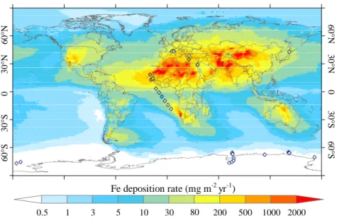
3.4 Mineral sources of Fe
Based on the soil mineralogical data (Journet et al., 2014), the estimated global total emission of Fe from mineral
sources ranged from 34.4 to 54.2 Tg yr−1 for 2000–2011,
with an average emission of 41.0 Tg yr−1. The modelled
average global total emission of dust for 2000–2011 was
1040 Tg yr−1, close to the median of 14 AeroCom Phase I
models (1120 Tg yr−1)(Huneeus et al., 2011). Our estimated
Fe emission from dust is lower than the 55–74 Tg yr−1
E m is sion of Fe ( Tg yr -1 ) 0 0.06 0.03 0.04 0.02 0.01 1960 1970 1980 1990 2000 Wildfires China A Other Europe 0 8 4 6 2 1960 1970 1980 1990 2000 Wildfires Africa NA SA Africa NA SA India Other Asia Russia Oceania China Other Europe India Other Asia Russia Oceania 0.05 B Figure 4
Figure 4. Temporal trends of Fe emissions of fine (PM1)(a) and medium-to-coarse (PM1−10and PM>10)(b) particles from combustion
sources from 1960 to 2007. Fe emissions from wildfires are shown separately with energy-related activities separated by region (NA for North America and SA for South America).
A
0.5 1 5 10 50 100 500 1000 3000
B
-1000 -100 -50 -10 10 50 100 500 1000
Fe emission density (mg m-2 yr-1) Fe emission density (mg m-2 yr-1)
-500 Global total: 41.0 Tg/yr Global total: +2.5 Tg/yr Sahara Desert Arabian Desert Takla-Makan Gobi Figure 5
Figure 5. Average Fe emission from dust sources for 2000–2011 using the new mineralogical data set (a) and the difference of average Fe
emission from dust sources for 2000–2011 using the new mineralogical data set relative to that using a constant Fe content (3.5 %) (b). A positive value in (b) indicates a larger emission density by using the new mineralogical data set.
the emission of dust is larger in the models used by these authors. For example, the model used by Luo et al. (2008)
simulated a total dust emission of 4313 Tg yr−1higher than
other 13 AeroCom Phase I models (Huneeus et al., 2011), including LMDz-INCA. However, the dust emission is very size-dependent, and the emissions should be evaluated by prescribing the size distribution in source regions to the trans-port models.
The average Fe emission density from mineral sources for 2000–2011 is mapped in Fig. 5a. The major source regions include the Sahara Desert, southern Africa, the Middle East, northwestern China, southwestern North America, southern South America, and western Australia. The estimated Fe emission map based on the new soil mineralogical data set (Journet et al., 2014) is also compared to that derived using a constant Fe content (3.5 %) (Fig. 5b) as measured by Taylor and McLennan (1985) and widely used in other models (Luo et al., 2008; Mahowald et al., 2009; Ito, 2013). The new min-eralogical data set led to a larger Fe emission density over the Sahara, Arabian and Takla-Makan deserts, and a lower Fe emission density over the Gobi Desert, reflecting the dif-ference of Fe content of dust relative to 3.5 % (Fig. S2).
3.5 Comparison of Fe emissions with previous studies Table 2 summarizes the comparison of our estimations of Fe emissions with previous studies (Bertine and berg, 1971; Luo et al., 2008; Ito, 2013). Bertine and Gold-berg (1971) estimated the emissions of 51 trace elements into
the atmosphere from fossil fuel combustion (1.4 Tg yr−1for
1967) based on a mass-balance method similar to ours. How-ever, due to a lack of measurement data at the time, they as-sumed that 10 % of all trace elements in fuels was transferred to the atmosphere. This rate is lower than the 30–45 % mea-sured for Fe in recent studies (Yi et al., 2008; Font et al., 2012; Tang et al., 2013). The estimate by Bertine and Gold-berg (1971) for the same year (1967) is within the uncertainty
range of our estimate (1.2–7.2 Tg yr−1as 90 % confidence),
but half of our central estimate (3.0 Tg yr−1)after accounting for different removal efficiencies by particle size and control device.
Luo et al. (2008) and Ito (2013) have estimated Fe emissions from the combustion of fossil fuels, biofuels
and biomass burning in fine (PM1) and medium
parti-cles (PM1−10). Their estimates of the total Fe emissions
es-timates (1.6 for 1996 and 1.3 Tg yr−1 for 2001 with a 90 % confidence range of 0.7–3.8 and 0.6–3.1, respectively). For fossil fuels, Luo et al. (2008) and Ito (2013) estimated Fe emissions based on the particle emission factors and the Fe contents of particles. Their estimates of fossil fuel emissions
(0.51 for 1996 to 0.66 Tg yr−1 for 2001) are close to the
lower bound in the uncertainty range of our estimates (0.6–
2.5 Tg yr−1as 90 % confidence for 1996 and 0.4–1.8 Tg yr−1
for 2001) and lower than our central estimates (1.2 and 0.9 Tg yr−1for the two years, respectively) for the same size class (Table 2). In the method used by Luo et al. (2008) and Ito (2013), the Fe contents of particles are measured in very few studies. For example, for coal burnt in power plants and industry, there are only three measurements in the USA which were used by Luo et al. (2008), reporting an Fe con-tent of 4.5–7.6 % in fine particles and 8.1–9.4 % in coarse particles (Olmez et al., 1988; Smith et al., 1979; Mamane et al., 1986). In addition to large uncertainty in sample collec-tion (Hildemann et al., 1989), the variacollec-tion of Fe content in particles is large. The measured Fe content in coal fly ash generated by the combustion of bituminous coal in Shanxi Province, China is 10.2–11.9 % (Fu et al., 2012), 40 % higher than the values used by Luo et al. (2008) and Ito (2013). A larger Fe content than that used by Luo et al. (2008) and Ito (2013) was also found for oil/biofuel fly ashes in the mea-surement by Fu et al. (2012). The large variation of Fe con-tent of particles explains part of the underestimation in the es-timates by Luo et al. (2008) and Ito (2013). In addition, Luo et al. (2008) and Ito (2013) estimated that the Fe emission
ratio between PM1and PM1−10is 1 : 6, compared to 1 : 24
in this study. The emission ratios used by Luo et al. (2008) and Ito (2013) were taken from Bond et al. (2004), which pertained to carbonaceous matter in fine particles but was not justified for Fe (mainly in coarse particles). For biomass burning, our central estimates of the total Fe emissions are lower than that by Luo et al. (2008) and Ito (2013). Luo et al. (2008) applied a globally constant Fe : BC emission ratio based on the slope of Fe and BC concentrations observed for aerosols in the Amazon Basin. Note that the dust and plant material entrained in fires can contribute to the Fe concen-trations in the atmosphere, as noticed by Luo et al. (2008). As a result, their estimates include the pyro-convection of Fe from soils and plant materials. In contrast, our estimate is based on the mass balance of Fe from the burnt fuels. This might explain partly why our estimate of the biomass burning emissions of Fe is lower than that in previous studies (Luo et al., 2008; Ito, 2013). Although our estimate provides an ex-plicit source attribution of Fe, which is useful for modelling the Fe solubility, it underestimates the total sources. We pro-pose that the emissions of Fe by pyro-convection in the fires should be estimated separately in the future.
In a recent study focused on East Asia (Lin et al., 2015), the emission of Fe from combustion sources in East Asia
in 2007 was estimated to be 7.2 Tg yr−1, far higher than all
other studies (Luo et al., 2008; Ito, 2013) and the central
es-timate in our study (1.6 Tg yr−1, with a 90 % confidence of
0.66–3.84). The authors used an alternative method to
esti-mate the emission of Fe based upon the sulfur dioxide (SO2)
emissions and the ratio of sulfur and Fe content in fuels. As pointed out by the authors, the emission of Fe from iron and steel industries is likely to be more important than previously thought. However, the authors also pointed out a notable un-certainty in their estimate because some parameters (e.g. the ratio of bottom ash to fly ash) are very uncertain due to the lack of measurements (Lin et al., 2015). The value taken for the ratio of bottom ash to fly ash in that study is from a single measurement that took place in Taiwan (Yen, 2011). Due to the lack of a sufficient number of measurements for some pa-rameters, our method cannot be applied to estimate the global Fe emission from the individual sector of iron and steel in-dustries. These remarks show that measurements are urgently needed to constrain the iron content of aerosols emitted from the iron and steel industries as well as other sectors.
4 Modelling of Fe concentrations
4.1 Spatial distribution of Fe concentrations in surface air
Based on the emissions of Fe from combustion sources as an average for 1990–2007 and mineral sources as an aver-age for 2000–2011, the global distribution of annual mean Fe concentrations attached to aerosols in surface air was de-rived (Fig. 6).
Globally, Fe emissions were much higher from
min-eral sources (41.0 Tg yr−1) than from combustion sources
(5.3 Tg yr−1). The modelled spatial distribution of Fe
con-centrations in surface air was thus dominated by mineral sources, in agreement with previous studies (Luo et al., 2008; Mahowald et al., 2009; Ito, 2013). Large Fe concentra-tions (> 1.0 µg m−3)are simulated over northwestern Africa, southwestern North America, western China, the Middle East, southwestern Africa and central to northern Australia. In addition to these continent regions, large Fe concentrations (> 0.1 µg m−3)are found over a large region of the Atlantic
Ocean from 0 to 30◦N due to the outflow of dust from the
Sa-hara Desert, and large Fe concentrations (> 0.5 µg m−3)are found over the Arabian Sea and the Indian Ocean due to the outflow of dust from the Arabian, Lut and Thar deserts. 4.2 Evaluation of Fe concentrations in surface air The Fe concentrations attached to aerosols in surface air
sim-ulated for pixels of 0.94◦latitude by 1.28◦ longitude were
evaluated by 529 measurements obtained between 1990 to 2007. These measurements include data compiled by Ma-howald et al. (2009) and Sholkovitz et al. (2012) and our collation of data from peer-reviewed studies (Table S2). The modelled Fe concentrations attached to aerosols in surface air, averaged for the months in the year of measurements,
5 1 0.5 0.1 0.001 0.01 3 10 50 60 °S 60 °N 30 °N 0 ° 30 °S 60 ° S 60 ° N 30 ° N 0° 30 ° S Thar Desert Sahara Desert Arabian Desert Lut Desert
Fe concentration in surface air (μg m-3)
Figure 6
Figure 6. Distribution of annual mean concentrations of Fe attached to aerosols in surface air. A total of 529 measured Fe concentrations
compiled by Mahowald et al. (2009) and Sholkovitz et al. (2012) and collected in this study (Table S3) are shown as circles, and a total of 296 Fe concentrations measured by Baker et al. (2013) over the Atlantic Ocean are shown as triangles.
Table 3. Statistics for the comparison of modelled and observed Fe
concentrations. N , sample size; F2and F5, fractions of stations with
deviations within a factor of 2 or 5, respectively; NMB, normalized mean bias. The values in parentheses show the indicators when the combustion sources are not included.
N F2(%) F5(%) NMB (%) Indian Ocean 61 30 (30) 75 (75) −68 (−68) Atlantic Ocean 224 64 (63) 83 (79) 15 (14) Pacific Ocean 126 52 (48) 69 (67) −66 (−69) South Ocean 47 47 (36) 53 (43) −44 (−79) East Asia 32 84 (13) 100 (31) −1.4 (−78) South America 4 75 (50) 100 (50) −73 (−91) North America 12 83 (33) 100 (67) −39 (−66) Mediterranean 23 61 (57) 87 (87) 24 (16) All regions 529 57 (49) 78 (70) −14 (−32)
are plotted against the measured concentrations after scaling the Fe concentrations from combustion sources (Sect. 2.7; Fig. 7a). The simulated Fe concentrations were grouped into the same size range as measurements if the size was speci-fied in the measurements; otherwise they were computed as total concentrations. The modelled spatial pattern matched
the observations (r2=0.53). Mahowald et al. (2009)
com-pared modelled annual mean Fe concentrations to measure-ments. They pointed out that the daily measurements from cruises are not as representative as the long-term station mea-surements. Similarly, a better agreement can be achieved if all cruise measurements are excluded in the comparison (r2=0.68) in our study (Fig. 7b).
M od el led Fe ( µg m -3) Measured Fe (µg m-3) 0.00010.001 0.01 0.1 1 1 0.0001 0.001 100 0.1 0.01 100 r2=0.53 Measured Fe (µg m-3) 0.00010.001 0.01 0.1 1 100 r2=0.68 Atlantic Ocean Pacific Ocean Indian Ocean Southern Ocean Mediterranean East Asia North Ame. South Ame. 1 0.0001 0.001 100 0.1 0.01 Long-term measurements sites Cruise measurements A B 10 10 10 10 Figure 7
Figure 7. Comparisons of modelled and observed Fe concentrations
by region (a) and measuring type (b). The modelled concentrations are averaged for the months in the year of measuring. The fitted curves for all stations in (a) and long-term measurement stations in
(b) are shown as red dashed lines, with coefficients of determination
(r2)listed. The 1 : 1 (solid), 1 : 2 and 2 : 1 (dashed), and 1 : 5 and 5 : 1 (dotted) lines are shown.
Three statistical metrics were used to evaluate the model performance (Table 3): the fraction of stations with a devi-ation within a factor of 2 (F2)or 5 (F5)and the normalized mean bias (NMB). Globally, 57 and 78 % of the stations were associated with deviations within factors of 2 and 5, respec-tively, with an NMB of −14 %. The model and observations agreed well for East Asia and the Atlantic Ocean, with de-viations within a factor of 2 for 84 and 64 % of stations, respectively. The model overestimated Fe concentrations at some stations over the Atlantic Ocean and the Mediterranean Sea. The model used only one major mode for dust (an initial MMD of 2.5 µm, and a fixed geometric σ = 2.0), which
re-produces the long-range transport and dust optical thickness over the ocean (Schulz et al., 1998). Without more detailed size bins, we assumed that the Fe content of dust and the Fe content of soil in the clay fraction is the same. This as-sumption is a reasonable approximation for dust transported hundreds of kilometres away from the dust source regions (Formenti et al., 2014), because the lifetime of dust is much longer for the clay fraction (up to 13 days) than for the silt (4 to 40 h) and sand (approximately 1 h) fractions (Tegen and Fung, 1994). However, the mineralogy and therefore the den-sity of material are not well considered in this simplification. This assumption would lead to an overestimation of the Fe content of dust near the source regions due to the ignored contribution of Fe in the silt and sand fractions (which have lower Fe contents than clay) (Formenti et al., 2014). To il-lustrate this impact, the global distribution of Fe content in dust simulated by assuming that Fe content of emitted dust is equal to that in the clay fraction of soil is shown in Fig. S4. We can see that the Fe content in dust over the Sahara Desert is 4.5–5.5 %, which decreases with the distance to the Sa-hara Desert. According to a measurement at a site with a dis-tance of about 2000 km to the Sahara Desert, the Fe content in dust is 2.5–2.7 % when the dust is originated from local erosion and 4.3 % when dust is originated from the Sahara Desert (Formenti et al., 2014). In the model, the Fe content is 4.5–5.5 % over the Sahara Desert, which is higher than the measured 2.5–2.7%, and 4–5 % over the regions distant from the Sahara Desert, close to the measured 4.3 % in dust after a long-range transport from the Sahara Desert (Formenti et al., 2014). In addition, when compiling data in the mineral-ogy database, Journet et al. (2014) noticed that wet sieving is used to determine soil texture, leading to loss of soluble min-erals (e.g. calcite or gypsum) and a possible overestimation of the content of minerals rich in Fe such as hematite and goethite. This impact might also contribute to an overestima-tion of Fe content in dust. The overestimaoverestima-tion occurs mainly at stations near continents and the downwind of deserts in Fig. 6, indicating that the modelled Fe concentrations over the ocean were not excessively influenced. The model also underestimated Fe concentrations over the Pacific and South-ern Oceans, likely due to the uncertainty in dust emissions and to the transport errors in the Southern Hemisphere, as documented previously (Huneeus et al., 2011, Schulz et al., 2012). Dust emissions over regions of the Southern Hemi-sphere, such as southern South America and southeastern Africa, require additional investigations.
One should note that modelled monthly mean concentra-tions were compared to daily measurements at some sites (e.g. measured by cruises) due to a lack of detailed date in-formation in measurements. It also caused some discrepan-cies between model and observations. As pointed out by Ma-howald et al. (2009), some cruise measurements were sen-sitive to episodic dust events. Mahowald et al. (2009) com-pared the modelled annual mean Fe concentrations to daily measurements, leading to a potential deviation by a factor
0.001 0.01 0.1 1 10 255 260 265 270 275 280 285 F e con ce n tr at ion (μ g m -3) measured model (day) model (month) Day of year A
Baker et al., 2006 (JCR cruise)
r2 = 0.58 r2 = 0.49 0.001 0.01 0.1 1 10 5 10 15 20 25 30 35 40 45 50 measured model (day) model (month) Day of year B r2 = 0.66 r2 = 0.01 Chen and Siefert, 2004 (winter)
F e con ce n tr at ion (μ g m -3) 0.001 0.01 0.1 1 10 175 185 195 205 215 225 measured model (day) model (month) Day of year C r2 = 0.28 r2 = 0.31 Chen and Siefert, 2004 (summer)
F e con ce n tr at ion (μ g m -3) 0.001 0.01 0.1 1 10 105 110 115 120 125 130 135 140 measured model (day) model (month) Day of year D r2 = 0.10 r2 = 0.39 Chen and Siefert, 2004 (spring)
F e con ce n tr at ion (μ g m -3) E
Baker et al., 2006 (JCR cruise) Chen and Siefert, 2004 (winter) Chen and Siefert, 2004 (summer) Chen and Siefert, 2004 (spring) 20°S 50°N 80°W 5°W 40°N 30°N 20°N 10°N 10°S 0
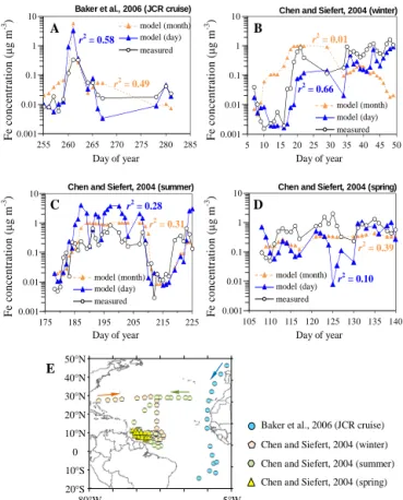
Figure 8. Comparisons of modelled and measured Fe
concentra-tions. The Fe concentrations were derived as monthly (blue tri-angles) or daily (orange tritri-angles) means from the model. (a) Fe measured in autumn 2001 (James Clark Ross (JCR) cruise) by Baker et al. (2006). (b) Fe measured in winter 2001 by Chen and Siefert (2004). (c) Fe measured in summer 2001 by Chen and Siefert (2004). (d) Fe measured in spring 2003 by Chen and Siefert (2004). (e) Locations of the cruise measurements (a–d).
up to 10. We also expected such a bias in this study, even though we were comparing modelled monthly Fe concentra-tions to all measurements. To address this influence, we com-pared modelled daily Fe concentrations to those from some cruise measurements with detailed date information available (Baker et al., 2006; Chen and Siefert, 2004). As illustrated in Fig. 8, particularly in Fig. 8a and b, the variation of daily con-centrations could be well captured by the model. These varia-tions were attenuated when using modelled monthly mean Fe concentrations. This agreement lends support to the estima-tion of annual mean Fe concentraestima-tions and thus Fe deposiestima-tion in our study.
4.3 Fe concentrations over the Atlantic Ocean
The modelled Fe concentrations attached to aerosols in air near the Atlantic Ocean were compared against 296 tran-sect cruise measurements for 2003–2008 (Baker et al., 2013) (Fig. 9). The zonal distribution of Fe concentrations was
Fe c on ce n tr ati on ( µg m -3 ) Latitude 40° -80° -40° 0° 1 0.0001 0.001 100 0.1 0.01 80° -60° -20° 20° 60° 10 Measured Modelled dust×2.12 dust×0.32 comb×2.27 comb×0.44 uncertainty of dust
Figure 9. Zonal distribution of modelled (cyan dots) and measured
(black dots) Fe concentrations attached to aerosols in surface air over the Atlantic Ocean from 70◦S to 60◦N. The solid lines with circles show the modelled (blue) and measured (black) Fe concen-trations as geometric means in each band with error bars for the geometric standard deviations. As sensitivity tests, Fe concentra-tions from mineral sources were scaled by factors of 0.32 and 2.12 (solid and dashed red lines) as 90 % uncertainties in dust emis-sions (Huneeus et al., 2011) and Fe concentrations from combustion sources were scaled by factors of 0.44 and 2.27 (solid and dashed green lines) as 90 % uncertainties in Fe emissions from combustion.
model overestimated the Fe concentrations in the band
be-tween 10 and 20◦N, because Fe content of the clay fraction
was extrapolated to all dust types, leading to an overestima-tion of Fe concentraoverestima-tions at locaoverestima-tions near dust source re-gions (see the discussion above). In addition, the model un-derestimated Fe concentrations by a factor of 2 at stations
in the band between 40 and 70◦S, and this model–data
mis-fit could be reduced when the modelled concentrations were scaled by a higher dust emission in a sensitivity test (Fig. 9), confirming the high degree of uncertainties in dust emissions and transport in the Southern Hemisphere.
The seasonality of modelled Fe concentrations at two long-term monitoring stations on the western margin of the Atlantic Ocean (Bermuda and Barbados) was compared to the observations, collected between 1988 to 1994 during the AEROCE program (Arimoto et al., 1992, 1995, 2003; Huang et al., 1999) and compiled by Sholkovitz et al. (2009). As shown in Fig. 10, the observed seasonal variations of Fe con-centrations at these two stations were well represented by the model, with peaks in summer corresponding to dust storms in the Sahara Desert.
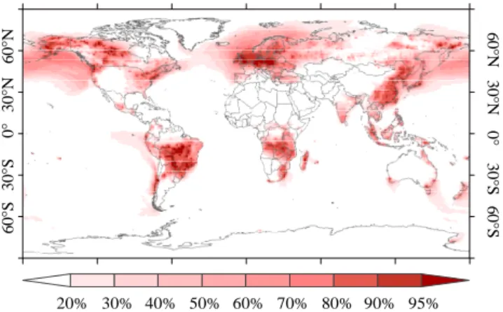
4.4 Role of the combustion sources
The estimated total emissions and the spatial distributions of Fe from combustion sources differed from those of previous studies (Table 2 and Fig. 3). The contribution of combustion sources to the Fe concentrations attached to aerosols in sur-face air is shown in Fig. 11. Large contribution of combus-tion sources (> 80 %) is found in western Europe, southeast-ern and northeastsoutheast-ern China, southsoutheast-ern Africa, central South
Jan Feb Mar Apr May Jun Jul Aug Sep Oct Nov Dec Jan Feb Mar Apr May Jun Jul Aug Sep Oct Nov Dec
Fe c once nt rat ion ( µ g m -3) 0.001 10 0.1 0.01 1 A B Measured Fe_total Fe_dust
Figure 10. Seasonality of Fe concentrations attached to aerosols
in surface air at Bermuda (32.2◦N, 64.5◦W) (a) and Barbados (13.2◦N, 59.3◦W) (b) on the western margin of the Atlantic Ocean. Modelled Fe concentrations are derived from all sources (Fe_total) and from mineral sources only (Fe_dust) as medians of all days of each month of 2005. Measured Fe concentrations are shown as the medians (circles) for 1988–1994 with the ranges between the 10th and 90th percentiles (error bars).
80% 60% 50% 40% 20% 30% 70% 90% 95% 60 °S 60 °N 30 °N 0 ° 30 °S 60 ° S 60 ° N 30 ° N 0° 30 ° S
Figure 11. Relative contribution of combustion sources to the
mod-elled Fe concentrations attached to aerosols in surface air.
America and eastern and northern North America, in agree-ment with the spatial distribution of combustion emissions.
To evaluate our estimation of the combustion sources of Fe, we divided all stations used in Sect. 4.2 into four groups based on the contribution to Fe concentrations by combus-tion sources. We plotted the modelled Fe concentracombus-tions with or without combustion sources against the observations (Fig. 12). The model can capture the observed Fe concen-trations at 53 stations with combustion contributions larger than 50 % well, with an average deviation of a factor of 1.5. The spatial pattern of Fe concentrations at these 53 stations is
also well captured (r2=0.73), lending good support to our
new estimation of Fe emissions from combustion sources. The scatter for stations with a smaller combustion contribu-tion indicates a higher uncertainty in mineral sources of Fe than combustion sources.
Due to too heavy computational load, we modelled the Fe concentrations from combustion in a typical year using the average Fe emissions during 1990–2007, and compared them with measurements during 1990–2007 by scaling the mod-elled Fe concentrations from combustion to a specific year with the temporal change of emissions at each site (Sect. 2.7).
M od el le d Fe ( µg m -3) Measured Fe (µg m-3) 0.00010.0010.01 0.1 1 100 Measured Fe (µg m-3) 0.00010.001 0.01 0.1 1 100
A. with combustion B. without combustion
Ratio (#) G1: 20.6 (53) G2: 2.4 (25) G3: 4.0 (76) G4: 1.2 (375) Ratio (#) G1: 1.5 (53) G2: 2.0 (25) G3: 3.2 (76) G4: 1.1 (375) r2=0.73 r2=0.40 1 0.0001 0.001 100 0.1 0.01 10 10 10 1 0.0001 0.001 100 0.1 0.01 10
Figure 12. Plots of modelled and measured Fe concentrations
at-tached to aerosols in surface air with (a) or without (b) combus-tion sources. All stacombus-tions were divided into four groups based on the contribution of combustion sources: G1, contribution ≥ 50 % (blue triangles); G2, 30 % ≤ contribution < 50 % (red triangles); G3: 15 % ≤ contribution < 30 % (green triangles); G4, contribu-tion < 15 % (grey squares). The ratios between measured and mod-elled concentrations as geometric means are listed with the number of stations in parentheses for each group. The fitted curves for the G1 stations are shown as blue lines with coefficients of determina-tion (r2).
To investigate the influence of this scaling process, we com-pared the modelled Fe concentrations without scaling among the four groups of sites (see results in Fig. S5). As a result, without this scaling, there is very minor change in the com-parison between the modelled and observed Fe
concentra-tions with r2 change from 0.73 to 0.72. This indicates that
the variation of Fe concentrations among the measuring sites is dominated by the spatial variation of Fe concentrations. 4.5 Effect of the new mineralogical database
Figure 13 shows the difference in modelled Fe concentra-tions using the new mineralogical data (Journet et al., 2014) relative to that using a constant Fe content in dust (3.5 %), as widely adopted (Luo et al., 2008; Ito, 2013). The new min-eralogical data increased the global total Fe emission from mineral sources from 38.5 to 41.0 Tg yr−1, with a relative dif-ference ranging from −60 to +30 % regionally (Fig. 5). Iron emissions were lower over the Takla-Makan and Gobi deserts (Fig. 5), leading to lower Fe concentrations over East Asia and the downwind regions over the northern Pacific Ocean. In contrast, Fe emissions were higher over the Sahara Desert and the deserts in the Middle East, southern Africa and cen-tral Auscen-tralia (Fig. 5), leading to higher Fe concentrations over the Atlantic and Southern oceans.
The effect of the new mineralogical database on the model–observation comparison at all stations used in Sect. 4.2 is shown in Fig. 14. All stations were divided into four groups based on the relative differences in Fig. 13. The influence was not very significant. There are 49 stations with a relative difference larger than 30 %, where the model bias was reduced from 40 to 20 %. The new mineralogical data also led to modest improvements in the comparison of
18% 6% 0 -10% -60% -30% 14% 26% 30% Takla-Makan Sahara Desert GobiDesert 60 °S 60 °N 30 °N 0 ° 30 °S 60 ° S 60 ° N 30 ° N 0° 30 ° S
Figure 13. Relative differences in simulated Fe concentrations
at-tached to aerosols in surface air when using the new mineralogical data and prescribing a constant Fe content in dust (3.5 %). A posi-tive difference indicates a higher Fe concentration when using the new mineralogical data.
M od el le d Fe ( µg m -3) Measured Fe (µg m-3) 0.00010.001 0.01 0.1 1 1 0.0001 0.001 100 0.1 0.01 100 Measured Fe (µg m-3) 0.00010.001 0.01 0.1 1 100 Ratio (#) G1: 1.4 (49) G2: 1.1 (158) G3: 1.5 (131) G4: 2.0 (191) Ratio (#) G1: 1.2 (49) G2: 0.8 (158) G3: 1.3 (131) G4: 2.0 (191)
A. with mineralogy B. without mineralogy 10 10 10 1 0.0001 0.001 100 0.1 0.01 10
Figure 14. Plots of modelled and measured Fe concentrations
at-tached to aerosols in surface air. The Fe content of dust was calculated from the new mineralogical data (a) or prescribed as 3.5 % (b). All stations were divided into four groups based on the relative differences between (a) and (b): G1, difference ≥ 30 % (blue triangles); G2, 20 % ≤ difference < 30 % (red triangles); G3: 10 % ≤ difference < 20 % (green triangles); G4, difference < 10 % (grey squares). The ratios between measured and modelled concen-trations as geometric means are listed with the number of stations in parentheses for each group.
elled and observed Fe concentrations in surface air over the Atlantic Ocean at all stations used in Fig. 9 of Sect. 4.3, with a slight improvement of the underestimation at latitudes
be-tween 40 and 70◦S (Fig. S6). The limited improvement
ob-tained using the state-of-the-art mineralogical database im-plied that other factors, such as the dust emission uncertain-ties and the transport errors, influenced the estimation of Fe from mineral sources. Further studies are needed to constrain the dust emissions in the Southern Hemisphere in the model (Tagliabue et al., 2009; Schulz et al., 2012). The new min-eralogical data provided information on the chemical form of the Fe in dust (Journet et al., 2014), which will help the modelling of Fe solubility.