HAL Id: hal-00489507
https://hal.archives-ouvertes.fr/hal-00489507
Submitted on 5 Jun 2010
HAL is a multi-disciplinary open access
archive for the deposit and dissemination of
sci-entific research documents, whether they are
pub-lished or not. The documents may come from
teaching and research institutions in France or
abroad, or from public or private research centers.
L’archive ouverte pluridisciplinaire HAL, est
destinée au dépôt et à la diffusion de documents
scientifiques de niveau recherche, publiés ou non,
émanant des établissements d’enseignement et de
recherche français ou étrangers, des laboratoires
publics ou privés.
A group model for stable multi-subject ICA on fMRI
datasets.
Gaël Varoquaux, Sepideh Sadaghiani, Philippe Pinel, Andreas Kleinschmidt,
Jean-Baptiste Poline, Bertrand Thirion
To cite this version:
Gaël Varoquaux, Sepideh Sadaghiani, Philippe Pinel, Andreas Kleinschmidt, Jean-Baptiste Poline, et
al.. A group model for stable multi-subject ICA on fMRI datasets.. NeuroImage, Elsevier, 2010, 51
(1), pp.288-99. �10.1016/j.neuroimage.2010.02.010�. �hal-00489507�
A group model for stable multi-subject ICA on fMRI datasets
G. Varoquaux
1,3∗, S. Sadaghiani
2,3, P. Pinel
2,3, A. Kleinschmidt
2,3, J.B. Poline
3, B. Thirion
1,3 1Parietal project team, INRIA, Saclay-ˆIle-de-France, Saclay, France,
2
INSERM unit´e 562, NeuroSpin, Saclay, France
3CEA, DSV, I
2BM, Neurospin, Saclay, France
†∗Corresponding author: Gael Varoquaux, [email protected], Laboratoire de Neuro-Imagerie Assiste par Ordinateur NeuroSpin CEA Saclay , Bt 145, 91191 Gif-sur-Yvette France
ABSTRACT
Spatial Independent Component Analysis (ICA) is an increasingly-used data-driven method to analyze functional Magnetic Resonance Imaging (fMRI) data. To date, it has been used to extract sets of mutually correlated brain regions without prior infor-mation on the time course of these regions. Some of these sets of regions, interpreted as functional networks, have recently been used to provide markers of brain diseases and open the road to paradigm-free population comparisons. Such group studies raise the question of modeling subject variability within ICA: how can the patterns representative of a group be modeled and estimated via ICA for reliable inter-group comparisons? In this paper, we propose a hierarchical model for patterns in multi-subject fMRI datasets, akin to mixed-effect group models used in linear-model-based analysis. We introduce an estimation procedure, CanICA (Canonical ICA), based on i) probabilistic dimension reduction of the individual data, ii) canonical correlation analysis to identify a data subspace common to the group iii) ICA-based pattern extraction. In addition, we introduce a procedure based on cross-validation to quantify the stability of ICA patterns at the level of the group. We compare our method with state-of-the-art multi-subject fMRI ICA methods and show that the features extracted using our procedure are more reproducible at the group level on two datasets of 12 healthy controls: a resting-state and a functional localizer study.
Introduction
Much of our understanding of brain function gained through functional Magnetic Resonance Imaging (fMRI) has been derived by correlating experimental signals of task-driven activation with external stimuli or events. Yet, the covariance structure of the fMRI signal holds as much information as the paradigm. Indeed at the scale of func-tional neuroimaging, positive correlations between distant regions induced by the coordination of distributed neuronal activity in a particular experimental context may provide a fundamental insight into brain function. Pioneered by Biswal et al.[1995], studies of paradigm-free functional connectivity investigate correlations in the BOLD (Blood Oxy-gen Level Dependent) time series. Such correlation studies have been decisive in identifying large functional networks of distant regions[Cordes et al., 2000, Greicius et al., 2003]. It has been established that the functional connectiv-ity signals observed in fMRI contains neuronal information beyond physiological or scanner noise [Laufs et al.,2003, Shmuel and Leopold, 2008], so that part of these signals can be considered a trace of underlying neuronal activity. In addition, recent work suggests that correlations in the functional signal are shaped by the anatomical connectivity structure [Greicius et al.,2008,Honey et al., 2007, Skudlarski et al.,2008,van den Heuvel et al.,2009].
Analysis of the correlation structure of the BOLD signal reveals large-scale patterns of correlated activity [Biswal et al., 1995, Lowe et al., 1998] and is expected to help understand the subdivision of the brain into cogni-tive systems that have coherent activity across time. These systems may be labeled as networks assuming that they
result from underlying brain connections [Bullmore and Sporns,2009,Honey et al.,2007] and serve distinct functions [Fox and Raichle, 2007, Smith et al.,2009].
The study of brain function through functional-connectivity mapping can be carried out without requiring the subject to perform a specific task. The so-called resting-state protocols can be easily applied, and are especially useful to include impaired subjects in a multi-group analysis. The networks identified by such experiments can give insights into the mechanisms of brain diseases and their modifications in pathological situation can serve as biomarkers to aid in clinical diagnosis [Garrity et al., 2007,Greicius,2008, Greicius et al., 2004,Mohammadi et al., 2009, Wang et al., 2006]. Recently,Seeley et al. [2009] have shown that large-scale brain networks of co-activation are adequate neuro-physiological units to study the impact of neuro-degenerative diseases.
The study of the correlation structure of brain activity is plagued by the size of the data: an fMRI dataset comprises more than 10 000 time series associated with the various voxels, which yield millions of possible pair-wise correlations. Functional-connectivity analysis has been pioneered through seed-based studies [Biswal et al., 1995, Cordes et al., 2000,Fox et al.,2005] that potentially uncover large-scale networks of brain activity correlated with a user-specified seed region. This approach, although very successful, is limited by the prior choice of seed regions of interest. Various clustering techniques [Cordes et al., 2002, Golland et al.,2007,Thirion et al.,2006] have been used to automatically define the regions or signals of interest. However, spatial ICA [Kiviniemi et al., 2003, McKeown et al., 1998] is, to date, the most popular method for identifying meaningful patterns in correlation studies without prior definition of any target region. The patterns extracted by ICA are usually easy to interpret in a cognitive neuroscience context, as they are most often well-contrasted, indicate different underlying physiological, physical, and cognitive processes, and can often be related to networks observed in different contexts, such as in seed-based analysis, or cognitive networks known from the literature [Smith et al.,2009].
ICA extracts salient patterns that are embedded in the data, and are thus considered as important to describe it. It is a purely data-driven method based on a loosely-constrained data model; as a consequence, statistical significance of the extracted patterns remains unclear. In particular, there is no simple way to extrapolate from findings obtained in one dataset to other datasets, even if these are sampled from the same population. In the context of group analysis, statistically well-controlled seed-based studies have shown that the BOLD signal contains patterns of correlation that are highly reproducible across subjects, including in resting-state experiments [Shehzad et al., 2009]. Similarly, some patterns extracted from resting-state fMRI datasets by an exploratory ICA approach are consistent at the group level [Damoiseaux et al., 2006] and have been used as biomarkers for population comparison [Garrity et al., 2007, Sorg et al.,2007].
However, ICA patterns can be relatively sensitive to mild data variation. Various, often non-overlapping, ICA patterns of group-level coherent activity have been reported, from resting-state data [Beckmann et al., 2005, Damoiseaux et al., 2006, Kiviniemi et al., 2003, Perlbarg et al., 2008], and in task-based experiments [Beckmann and Smith,2005,Calhoun et al.,2001]. Probabilistic models have been used to provide pattern-level noise-rejection criteria [Beckmann and Smith,2004] or goodness-of-fit measures of the model [Guo and Pagnoni,2008], but still they do not provide pattern-level significance testing. The uncontrolled variability of the individual patterns is detrimental to population studies: there is no established framework for between-group comparison or inference on
ICA maps.
ICA being an exploratory analysis technique that estimates a mixing model specific to the data, it is not meaningful to compare directly patterns estimated on different individual subjects. On the contrary, group-level patterns can be specialized to each subject [Calhoun et al., 2001, Filippini et al., 2009]. Different strategies have been adopted for group-level extraction of ICA patterns. Patterns estimated at the subject level can be merged to form group maps [Esposito et al.,2005,Perlbarg et al.,2008] although this is a challenging task because the correspondence of individual maps may be hard to assess and the merging operation is difficult to model from a statistical point of view. Individual-subject volumes can be concatenated along the time axis to apply the ICA algorithm on the group data [Calhoun et al., 2001]. Finally,Beckmann and Smith[2005] have developed a tensorial extension of ICA that estimates patterns across subjects sharing the same time course throughout the experiment.
In this paper, we present a novel group model for multivariate patterns in fMRI volumes and an associated estimation procedure to extract group-level ICA maps modeling subject variability. The strength of this method called CanICA lies in the identification of a subspace of reproducible components across subjects using generalized canonical correlation analysis (CCA). Combined with an explicit noise model and resampling procedure, this enables automatic selection of the number of components. In addition, we introduce a cross-validation procedure and metrics to compare the stability of a set of multi-subject patterns across different sub-populations. We compare our method to state-of-the-art fMRI group ICA methods with different group models: concatenation and tensorial group ICA approaches. We do not compare to merging procedures since they do not rely on a linear model between individual subject-level datasets and group-level Independent Components (ICs) and thus cannot be formulated with a spatially-resolved between-subject variability of group-level ICs. We show with cross-validation that features extracted by our method are more stable on a group of 12 controls, both in a resting-state experiment and in a traditional activation detection experiment with a known paradigm.
Theory
Spatial ICA model for fMRI data
ICA assumes that the observed data is the linear mixture of unknown base signals, that are recovered based on measures of statistical independence. The underlying model is that of blind separation of independent sources:
B= MA, (1)
where the rows of the matrix B are the observed patterns, and those of A form the patterns corresponding to the estimated independent sources, and M is a mixing matrix estimated by ICA. To set the notations, when considering spatial patterns or components, such as A or B, in this article, we will use npatterns× nvoxels-shaped matrices; npatterns
is a number that corresponds to the model order, or possibly the number of observations, depending on the context. Note however that the independence of the patterns extracted by ICA algorithms is not guaranteed in theory and rarely checked in practice, and that the independence criterion used to identify the components often boils down
to sparse component extraction [Daubechies et al., 2009]. There is no theoretical basis to consider that a pattern is representative of solely one independent process, for instance movement, although in practice ICA is so far one of the of factor analytic transformations [Langers, 2009] most suited to blind pattern extractions from fMRI data. In addition, it is not clear that, from a neuroscientific point of view, independence is the right concept to isolate brain networks, as no functional system is fully segregated.
The patterns B present in the acquired fMRI volumes are confounded by observation noise. As a result, the ICA mixing model is most often applied on a subset of the acquired signal, after an initial data-reduction step. In most ICA methods, this step is carried out using a Principal Components Analysis (PCA), the order of which thus determines the dimension of the signal subspace and thus the number of sources extracted by ICA. In the context of fMRI data analysis, a probabilistic PCA model can be used to introduce a noise model as the basis for this subspace selection [Beckmann and Smith,2004].
Existing group models for ICA on multi-subject fMRI data
ICA is a multivariate analysis technique: voxel-based time courses are not characterized as such, but as part of signal fluctuations in the entire brain. As a consequence, the voxel-level group models used in standard mass-univariate analysis –random effects or mixed effects– cannot be applied directly ICA patterns. Two main strategies have been used so far to extract group-level patterns for fMRI images.
A first approach, introduced by Calhoun et al. [2001], concatenates individual subject data and performs data reduction and ICA on the resulting dataset. Data reduction is done by PCA. Subject maps are obtained by applying the mixing model learned on the group to the data specific to a subject. The group model underlying the estimation procedure is that the images observed Y in the individual datasets are generated by a mixture of the group-level ICA patterns A with additional noise E:
P = MA (2)
Y = WP+ E (3)
with Y = [YT
1, . . . , YTS]T the observed individual subjects images concatenated along the time axis, and E the noise. W
gives a subject-specific set of loadings and P are the principle components spanning the inter-subject signal subspace. This model consists in the addition of a subject-dependent observation noise in equation3to the ICA model (equations
2 or 1). The GIFT toolbox [Calhoun et al.,2001] (http://icatb.sourceforge.net/) and the MELODIC software used in ConcatICA mode [Smith et al.,2004] implement variations on this model. They differ in the way to represent the group-level patterns: GIFT uses a T-statistics-based thresholding on a random-effects analysis of the individually reconstructed maps {M−1W−1
i Yi, i= 1 . . . S}. This amounts to building a posteriori a hierarchical model with two
levels of variance. ConcatICA, on the other hand, directly thresholds the groups patterns (see further). In either case, the model is estimated in two steps, using principal component analysis (PCA) to solve equation 3, followed by a noiseless ICA algorithm to identify the independent components in equation2. In the actual implementations of the estimation of the group model in equation3, the generative model differ slightly from the model on a implementation
basis, as data reduction steps may be implemented via successive PCAs to limit the numerical size of each step. The tensorial extension to ICA developed byBeckmann and Smith[2005] uses a model inspired from PARAFAC [Harshman,1970]: the observed images Y are modeled as a trilinear combination of group-level independent patterns A, common time courses, and subject-specific loadings, with additional observation noise E:
Y= (M| ⊗ |N)A + E. (4)
Matrices M and N give the mixing of independent patterns across subjects and components. (.| ⊗ |.) is the Khatri-Rao product, which imposes a triple-outer-product relationship between subject components and group-level independent components: subject components share the same set of independent spatial patterns and time courses for each spatial map, but the contribution of each independent pattern varies from subject to subject. The hypothesis guiding the tensor ICA model is that, in a multi-subject experiment with external correlates, the time course corresponding to activation of cognitive networks is set by the experiment, and thus shared between subjects. On the other hand, tensor ICA may imply only a low degree of prevalence of the components with respect to the dataset at hand, because it allows arbitrary subject-level loadings on each of the independent components.
Guo and Pagnoni[2008] have described both approaches as special cases of a general decomposition model in which subject-specific images are a linear combination of group-level independent components:
Y= MA + E (5)
with Y = [YT
1, . . . YST]
T the group data matrix made of the time-wise concatenation of observed individual subjects
data. The Group-ICA model and the Tensor-ICA model can be seen as putting restrictions on the structure of the mixing matrix M. Guo and Pagnoni[2008] propose a more general estimation algorithm of an unconstrained mixing matrix with an expectation maximization (EM) algorithm, to learn the group structure associated via the data. The limitation of this EM approach is that it is based on modeling the histogram of the independent components with an mixture of an arbitrary number of Gaussian components.
Group comparison with ICA
While ICA is often used to compare functional connectivity between groups, the mixing model of ICA does not provide a natural statistical framework for comparing patterns estimated from different datasets, unlike the GLM framework. Two recent contributions have laid out statistical group-comparison procedures.
Guo and Pagnoni [2008] propose a goodness-of-fit measure for their mixture-of-Gaussian-based ICA generative model using an approximate likelihood ratio test to compare different mixing models and discriminate if a group is better modeled as a homogeneous population or as a set of different subgroups. However, this approach essentially assesses the amount of data variance fit by the model (which is measured by the likelihood ratio test) so that it may be systematically affected by dimension selection issues, while it assumes that the unmodeled variance is independent across voxels to allow tractable computations.
Rombouts et al. [2009] use Tensor-ICA and a two sample t-test on the loadings of the different group patterns between healthy controls and patients with dementia to identify the patterns represented unevenly in the two popu-lations.
The above procedures provide important indications on data structure, but they do not directly highlight the difference between groups in the individual ICs. Some of these individual patterns represent biologically-meaningful components and are used in cognitive studies and as biomarkers. There is thus a strong interest in basing group comparisons on the patterns themselves, rather than the complete mixing model, such as performed inGarrity et al. [2007],Greicius et al.[2004],Mohammadi et al.[2009]. The difficulty in comparing these patterns stems from the fact that the estimation performed by the ICA algorithm is not robust against mild data variation: some global differences may exist between two decompositions of datasets that resemble each other; for instance, an IC present in one dataset can show salient features that are separated into two components in another dataset, so that we may consider the IC as split into two in the other dataset.
Materials and methods
A multivariate extension of mixed-effects models
To achieve a better control on variability of the ICs due to individual difference between subjects, we introduce a generative model of the signal making the separation between subject-to-subject variability, and observation noise specific to a subject or a session. At the group level, we describe the BOLD signal by a set of patterns A corresponding to different independent components. These different components are extracted in a signal space common to the group and spanned by principal components B. The generative model relates these group-level patterns to the observed signal via different noise terms.
Generative model
Group-variability model The activity recorded on each subject s can be described by a set of subject-specific spatial patterns Ps, which are a combination of the group-level patterns B and additional subject-variability:
for each subject s, Ps= ΛsB+ Rs, (6)
with Λsa loading matrix giving how much each pattern is represented in subject s, and Rsa residual matrix giving
the deviation from the group patterns. In other words, a group description can be written considering the group of patterns (vertically concatenated matrices) P = {Ps}, R = {Rs}, and Λ = {Λs}, s = 1 . . . S,
P= Λ B + R. (7)
Λis a loading matrix relating the subject-level components for each subject to the group-level components. If there are ngrp components generating the signal at the group level, and each of the S individual datasets are described by
nsbj, the shape of the loading matrix Λ is (S · nsbj, ngrp) (see figure1for a diagram).
Observation model For each acquisition-frame time point the observed data is a combination of different subject-specific patterns Psconfounded by observation noise: let Ysbe the resulting spatial images in BOLD MRI sequences
for subject s (an nframes× nvoxels matrix), Es the observation noise, and Wsa loading matrix such that:
Ys= WsPs+ Es. (8)
Parallel to mixed-effect models
The generative model can be written in a non-hierarchical form as:
Y1 .. . Ys = W1 0 0 0 . .. 0 0 0 Ws Λ1 .. . Λs MA+ R1 .. . Rs + E1 .. . Es (9)
In the group ICA framework ofGuo and Pagnoni[2008],
Y= ˜MA+ ˜E (10) with M˜ = W1 0 0 0 . .. 0 0 0 Ws Λ1 .. . Λs M (11) and E˜ = W1 0 0 0 . .. 0 0 0 Ws R1 .. . Rs + E1 .. . Es (12)
In other words, the mixing matrix can be factored out in a subject-specific matrix and group-level matrix, and the rejected noise is the addition of two terms, a subject-specific one and a group-level one, that explain different components of the signal. If we compare the ICA analysis with a GLM analysis, as suggested inMcKeown et al.[1998], in equation10, ˜M corresponds to the design matrix, and ˜E to the residuals. We can see that the decomposition of these matrices in equations11and12can also be identified as the non-hierarchical expression of corresponding terms in a mixed-effect model (see for instanceFriston et al.[2005]).
Thus, the two-level group model exposed above can be seen as a multivariate formulation of mixed-effects models, often used in a standard univariate GLM-based analysis, as it models two sources of variance. However, it is not hypothesis-driven and does not rely on the knowledge of external correlates.
Estimation procedure
In this section, we describe the estimation procedure used to extract the patterns of interest from the data. The different variables estimated corresponding to the generative model are noted with a hat: if A is the population set
Figure 1: Diagram of the estimation procedure: successive estimation steps are applied from left to right, starting from individual datasets, to end with group-level independent components.
of patterns introduced in the model, ˆAdenotes the corresponding patterns estimated from the data. Figure1gives a diagram summarizing the model and the successive estimation steps.
Noise rejection using the generative model
We start from fMRI image sequences, for each subject, corrected for delay in slice acquisition and for motion, then registered to a common template space. We extract the time series corresponding to a mask of the brain, center and variance-normalize them, resulting in pattern matrices {Ys, s= 1...S}, with s corresponding to the subject index. We
separate reproducible group-level patterns from noise by estimating successively each step of the above hierarchical model.
Subject-level identification of observation noise First, we separate observation noise Es from subject-specific
patterns Ps as in equation (8), through principal component analysis (PCA). The principal components explaining
most of the variance for a given subject’s data set form the patterns of interest, while the tail of the spectrum is considered as observation noise.
Specifically, for each subject, we use a singular value decomposition (SVD) of the individual data matrix,
Ys= UsΣsVs. (13)
We retain the first nsbj(s) rows of Vsto constitute the patterns ˆPsand the first nsbj(s) columns of (UsΣs) give their
loadings ˆWsin the subject’s data, that can be interpreted as time courses of the components. The residual constitutes
the observation noise, ˆEs:
ˆ Ps = (Vs)1...nsbj, (14) ˆ Ws = (UsΣs)1...nsbj, (15) ˆ Es = Ys− ˆWsPˆs, (16)
Setting the number nsbj(s) of principal components to retain at the subject level is a difficult question and
not the main focus of this article. In general, this number can be selected by analyzing the individual datasets. We have found that with information-theoretic criteria initially used for model-order selection in PCA algorithms (Beckmann and Smith [2004],Calhoun et al.[2001],Minka[2001]), the number of identified sources is overestimated for long fMRI time series and many non-meaningful ICA components are extracted. Various studies have been con-ducted of the influence of PCA-model-order choice in fMRI ICA methods [Himberg et al.,2004,Kiviniemi et al.,2009, Li et al.,2007]. The optimal number of ICs has been empirically found to lie between 20 and 60 components depending on the dataset.
We use the resampling method described by Mei et al. [2008] in the context of statistical shape modeling. This method estimates the number of principal components necessary to model the data in the presence of Gaussian-distributed noise by assessing the stability of the subspaces spanned by the first nsbj(s) principal components. Mei et al.
[2008] showed empirically that it does not lead to diverging model order when new datasets are generated from the selected principle components with additional Gaussian-distributed noise. For more details on the model-order selection algorithm and its robustness to noise, we refer the reader toMei et al.[2008]. We apply this algorithm on the individual subject datasets, Ysafter the various prepocessing steps, as it is input in our group model. For computational reasons,
we estimate the subject-level number of components on only one subject’s data if all the individual datasets share the same acquisition parameters and length and use this parameter for all individual datasets: we assume that nsbj(s) is
independent of s, and we write nsbj.
Canonical correlation analysis to estimate the group-level patterns At the group level, we are interested in identifying the sub-space common to each subject’s patterns. For this purpose, we use generalized Canonical Correlation Analysis (CCA).
CCA is most often used to compare two multivariate datasets by finding the successive univariate components pairs of each dataset that maximize cross-correlation. The components pairs are called canonical variables, and the associated correlation is the canonical correlation. We use a generalization of CCA to multiple datasets [Kettenring, 1971,Krzanowski,1979]– in our case, one dataset per subject. We start from the different whitened datasets1Pˆ
s, and
concatenate them to form ˆP. We perform an SVD on ˆP:
ˆ
P= Υ Z Θ. (17)
where Υ and Θ are rotation matrices, and Z is the diagonal matrix of singular values. The rows of Θ form the canonical variables, in other words the inter-subject reproducible components, and the singular values on the diagonal of the matrix Z form the canonical correlations, which yield a measure of between-subject reproducibility. We retain the first ngrp vectors of Υ, the canonical weights forming the patterns of interest at the group level:
ˆ
Bs= (Υs)1...ngrp, (18)
1The singular value spectrum of ˆPs is made only of ones: ˆPsPˆT
s = 1. In other words, the amount of variance each IC wich accounts for at the subject level is not modeled at the group level: only the patterns are retained, ˆΣs is not considered.
We select the dimension ngrp by keeping only the canonical variables for which the corresponding canonical correlation
Zis above a significance threshold as described below.
The significance threshold on the canonical correlations is set by sampling a bootstrap distribution of the maximum canonical correlation using ˆEs, the subject-level observation noise identified previously, instead of the subject-level
components of interest ˆPs. Selected canonical variables have a probability p < 0.05 of being generated by data
consisting only of observation noise. This procedure corresponds thus to keeping only the group-level components more reproducible than observation noise. We give more details on this procedure in the supplementary materials.
The estimation procedure for the group-level subspace of interest is thus done by minimizing the amount of unexplained signal in each subject while using a fixed number of components, and then by maximizing the subspace stability at the group level. Both optimizations are performed using SVD. For each step, the unexplained variance is chosen based on a noise model.
Group-level independent components
The above estimation procedure selects group-level components B spanning the subspace of common patterns of activation. We apply FASTICA [Hyv¨arinen and Oja, 2000] on this subspace, to separate group-level independent sources A, estimating the mixing model1.
Finally, as the interesting features of the ICA patterns lie in blobs standing out from the background, it is im-portant to threshold the resulting map to keep only the tail of the intensity distribution2. For this, we use as
simple null-hypothesis distribution a normal distribution of unit standard deviation. Indeed, the FastICA algorithm works on whitened data (thus of isotropic unit variance) and estimates maximally non-Gaussian directions. As in Schwartzman et al. [2009], this null hypothesis models the central mode of the maps, and we select the voxels for which the absolute intensity exceeds a fixed threshold, that corresponds to a certain level of specificity with respect to null distribution. More complex thresholding approaches have been developed, for instance based on mixture modeling [Beckmann and Smith,2004]. Our method leads to fewer selected voxels on a pattern with very few salient features, such as on artifact patterns. In addition, it is consistent with the FastICA model.
The main differences of our estimation method compared to the most currently-used fMRI ICA methods (GIFT and MELODIC) are:
1. Model-order determination by rejecting components that can be generated by Gaussian noise.
2. Selecting a subspace of reproducible components at the group level using canonical correlation analysis as a device to separate subject-level observation noise for group variability.
3. Thresholding ICs based on the absolute value of voxel intensity.
In this article, we are mostly interested in discussing the importance of point 2, which is the expression of the group model used to describe between-subject variability.
2Although this is sometimes done implicitly by simply referring to the brain regions that stand out when looking at spatial maps, it is important to this do this reduction explicitly.
Cross-validation of group-level patterns
The use of ICA is motivated by the fact that the patterns extracted from the fMRI data display meaningful features in relation to our knowledge of functional neuroanatomy. The validation criteria for an ICA decomposition are unclear, as this algorithm is not based on a testable hypothesis. However, for the method to be usable in group studies, the features extracted from a group of healthy controls should be comparable between different subgroups of subjects, and generalize to different subgroups.
To test the reproducibility of the results across groups of subjects, we split our group of subjects in two and learn ICA maps from each sub-group: this yields the sets of patterns A1 and A2. We compare the overlap of thresholded
maps and reorder one set to match maps by maximum overlap. Reproducibility can be quantified by studying the cross-correlation matrix C = AT
1A2. For unit-normed components, Ci,j = 1 if and only if (A1)i and (A2)j are
identical.
To quantify the reliability of the patterns identified on the full datasets, we select for each pattern extracted from the full dataset the best matching one in the different subsets computed in the cross-validation procedure using Pearson’s correlation coefficient. Along with the extracted maps, we report the average value of this pattern-reproducibility measure.
Validation experiments: comparing to other methods We compare our method with state-of-the-art methods using different group-model estimation procedures: concatenation approaches using the implementations of the GIFT ICA toolbox [Calhoun et al.,2001] and the MELODIC software [Smith et al.,2004], as well as the tensor ICA model, also implemented in the MELODIC software [Beckmann and Smith,2005].
Also, to isolate the effect of separating subject-level variance from group-level variance in the estimation algorithm from implementation-specific details, we run a modified version of CanICA without the CCA step, retaining the subject-level variance Σsat the group level on the same datasets: equations 15and16are thus replaced by
˜
Ps = (ΣsVs)1...nsbj, (19)
˜
Ws = (Us)1...nsbj. (20)
With this estimation algorithm, the variance explained by the components at the subject level is carried on to the group level. This is analogous to a fixed-effect model.
As estimating larger numbers of independent components tend to explore less stable patterns, we run all analysis using the number of components estimated by CanICA. We perform cross-correlation analysis on the non-thresholded ICA maps, but also use each implementation’s thresholding algorithm to separate the features of interest. In an effort to separate the impact of the group model from the impact of the thresholding heuristic, we study reproducibility of non-thresholded maps, as well as thresholded maps, although non-thresholded maps can be considered as of little neuro-scientific interest. The mixture model implemented in MELODIC selects 3000 voxels on average on all the patterns. We set the specificity for the other methods to select the same average number of voxels. For GIFT, the thresholding is done on the t statistics maps generated by the algorithm. We threshold at |t| > 2.
Similarity measures for decompositions learned in different subjects We define two measures to quantify the stability of the subspace spanned by the components and the reproducibility of the maps. First, a measure of the overlap of the subspaces selected in both groups is given by the energy of the matrix, i.e. its Frobenius norm: E= tr (CTC). To compare this quantity for different subspace sizes, we normalize it by the minimum dimension of
the subspaces, d = min(rank A1,rank A2) (21) e = 1 dtr (C TC ). (22)
equantifies the reproducibility of the subspace spanned by the maps. For e = 1, the two groups of maps span the same subspace, although individual independent components may differ. If A1 and A2 have different dimensions, taking
the minimum dimension of both does not account for possible instability of patterns extracted from a group and not the other. However, the dimensionality as estimated by our procedure does not vary much over the cross-validation pairs (maximum 10% relative difference).
Second, we measure one-to-one reproducibility of maps. We reorder the matrix C by matching sequentially maximally mutually correlated components of A1and A2, considering the absolute value of the pair-wise correlation.
This procedure creates a reordered cross-correlation matrix ˜C with maximal matching values on the diagonal. If one of the two groups has more components than the other, we use the smallest of the two as a reference, and stop the matching procedure once all of its components have been matching. As a result, ˜C is a square matrix, that we populate with absolute values of pair-wise correlations. Although we acknowledge that this algorithm may not give the optimal matching in general, we observe that the solution is satisfactory in practice. We use the normalized trace of the reordered cross-correlation matrix,
t=1
dtr ( ˜C), (23)
as an overall measure of one-to-one overlap between matched pairs of components.
fMRI datasets
We apply the probabilistic ICA method described above to extract brain networks from two multi-subjects datasets: a group resting-state study and a functional localizer.
Resting-state data We use datasets from a resting-state experiment: subjects were blindfolded and instructed to keep their eyes closed. The resting state session was recorded as the first session preceding a series of cognitive experiments as part of a study not detailed here. At the time of resting-state data collection, subjects were naive with respect to the nature of the subsequent experiments. Twelve right-handed healthy volunteers (2 female; ages 19–30) gave written informed consent before participation in imaging on a 3T MRI whole-body scanner (Tim-Trio, Siemens, Erlangen). The study received local ethics committee approval. 820 EPI volumes (25 slices, T R = 1.5 s, T E = 30 ms, FOV 19.2 cm × 19.2 cm, 3 mm isotropic resolution) were acquired during a rest period of 20 minutes. A full description of the paradigm and the acquisition parameters can be found inSadaghiani et al.[2009].
Functional localizer data We used an event-related experimental paradigm consisting of ten conditions. Subjects were presented with a series of stimuli and were engaged in tasks such as passive viewing of horizontal or vertical checkerboards, left or right button press after auditory or visual instruction, computation (subtraction) after video or visual instruction and sentence processing, from the auditory or visual modality. Events were randomly occurring in time (mean inter stimulus interval: 3 s), with ten occurrences per event type (except button presses for which there are only five trials per session).
Two hundred right-handed subjects participated in the study. The subjects gave informed consent and the protocol was approved by the local ethics committee. Functional images were acquired on a 3T Bruker scanner using an EPI sequence (40 slices, T R = 2.4 s, T E = 60 ms, FOV 19.2 cm × 19.2 cm, 3 mm isotropic resolution). A session comprised 132 scans. The first four functional scans were discarded to allow the MR signal to reach steady state. The experimental paradigm and the acquisition parameters are described with more detail inPinel et al.[2007]. To balance the comparison with resting-state data, we first report reproducibility analysis on 12 subjects acquired consecutively. We also study reproducibility on a group of 62 subjects all acquired successively in time.
Preprocessing The above datasets were preprocessed using the SPM5 software (Wellcome Department of Cogni-tive Neurology; http://www.fil.ion.ucl.ac.uk/spm). After slice-timing interpolation and motion correction, cerebral volumes were realigned to the MNI152 inter-subject template and smoothed with a 5 mm isotropic Gaussian kernel. Voxels contained in a mask of the brain (approximately 40 000 voxels) were selected for pattern extraction using the CanICA procedure. We do not apply a frequency filter to the time-series, as we have found out that this yields ICs displaying better separation between brain networks and artifacts such as movement or blood-flow related patterns.
Results
Group-level patterns extracted
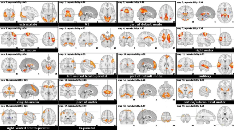
Resting-state dataset On the resting-state dataset, consisting of 820 scans, CanICA identified in average 50 non-observation-noise principal components at the subject level and a subspace of 42 reproducible patterns at the group level (see equation7). This number matches those commonly hand-selected by users in current ICA studies. Kiviniemi et al.[2009] reported 60 stable independent components and 42 brain networks in a study of group-level ICA patterns stability on a similar dataset. On this dataset made of long time sequences, model-evidence-based methods such as those used in Beckmann and Smith [2004] select 200 components at the subject level (or 340 when applied on smoothed data). Out of the 42 maps extracted by the CanICA, we identified by eye 26 putatively components as brain networks (Fig. 2). When using CanICA without CCA, we putatively identified only 11 components extracted as brain networks. Other components related to physiological noise or movement form patterns in the BOLD signal common to the group as they are related to reproducible anatomical features.
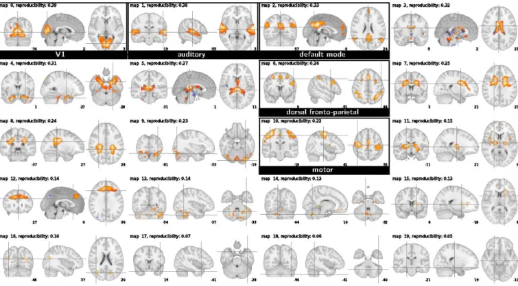
Functional localizer dataset On the functional localizer dataset, consisting of 150 scans, CanICA extracts 20 ICA patterns, out of which we identify 13 putative functional networks (see Fig. 3). When using equation20 instead of
Figure 2: The 42 ICA maps extracted by CanICA from the resting-state dataset (display in radiologic convention: the right hemisphere is on the left of the axial view). The maps are ordered by reproducibility (from left to right on each line, and top to bottom line after line). Maps corresponding to functionally plausible networks are in a black frame, whereas maps likely corresponding to artifacts are not framed. Extracted brain networks are labeled with the name of the general structure they can be related to.
Figure 3: The 20 ICA maps extracted by CanICA on the functional localizer dataset (radiologic convention).
MELODIC GIFT MELODIC CanICA CanICA TensorICA GroupICA ConcatICA no CCA CCA
Resting state Unthresholded ICA maps
e: subspace stability .47 (.06) .58 (.04) .58 (.04) .36 (.02) .71 (.01) t: one-to-one matching .36 (.03) .53 (.04) .51 (.04) .36 (.02) .72 (.05)
Thresholded ICA maps
t: one-to-one matching .35 (.02) .10 (.01) .50 (.03) .21 (.02) .62 (.04) Localizer
Unthresholded ICA maps
e: subspace stability .54 (.05) .25 (.03) .43 (.02) .35 (.01) .52 (.01) t: one-to-one matching .36 (.02) .34 (.04) .35 (.03) .37 (.02) .55 (.02)
Thresholded ICA maps
t: one-to-one matching .29 (.03) .02 (.01) .31 (.05) .26 (.03) .46 (.02)
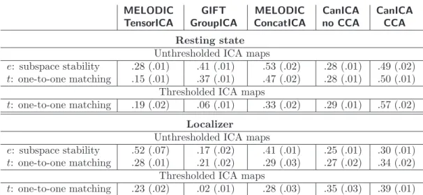
Table 1: Average reproducibility measures e and t for Group ICA, Tensor ICA and CanICA calculated on the half-split cross-correlation matrices, both for non-thresholded and thresholded maps. Numbers in parenthesis give the standard deviation across the different splits.
12 subjects 20 subjects 40 subjects 62 subjects
no CCA CCA no CCA CCA no CCA CCA no CCA CCA
Unthresholded ICA maps
e: subspace stability .35 (.01) .52 (.01) .36 (.01) .57 (.01) .42 (.01) .71 (.01) .50 (.01) .78 (.01) t: one-to-one matching .37 (.02) .55 (.02) .40 (.02) .57 (.03) .45 (.01) .68 (.03) .49 (.01) .72 (.03)
Thresholded ICA maps
t: one-to-one matching .26 (.03) .46 (.02) .29 (.02) .45 (.03) .33 (.02) .56 (.03) .38 (.03) .60 (.04)
Unthresholded Thresholded
RS Loc. RS Loc.
Matching above 50% 91% 64% 77% 44%
Matching below 25% 0% 2% 5% 25%
Matching above 75% 55% 19% 34% 28%
Table 3: Percentiles of maximum one-to-one matching between maps extracted with CanICA on two sub-group of 6 different subjects.
equation 15, i.e. without the whitening of the individual patterns imposed in the CCA, only 6 functional networks are identified (see supplementary materials).
Reproducibility results
The reproducibility metrics we obtained by cross-validation are reported in Table1. For the resting-state experiment, on non-thresholded maps, the GIFT and ConcatICA perform similarly with regards to subspace-stability, which can be explained by the fact that they implement similar group models. For this experiment, the reproducibility of the TensorICA model is not as good. Conversely, for the localizer experiment, the reproducibility of TensorICA is good. The assumption of the TensorICA model that networks share similar time courses across subjects is clearly more suitable for task-driven studies. The CCA-based estimation procedure of the two-level group model of CanICA yields the most stable subspace in both experiments. However, the relative performance of different methods changes between the two experiments that have very different signal length and TR.
Performance of the method with regards to one-to-one reproducibility of thresholded maps does not differ sig-nificantly from non-thresholded maps for all the methods using histogram-based thresholding. On the other hand, GIFT thresholds a t-statistic map over back-reconstructed subject-specific components, which is quite unstable across population splits. As a result, one-to-one matching of thresholded maps extracted by GIFT does not perform well. We also note that the independent components extracted from the functional localizer dataset are less contrasted than those extracted from the resting-state data because the number of volumes is smaller, and as a result thresholding has a more detrimental impact on stability.
The distribution of maximal component matching from one sub-group to another provides an assessment of the reproducibility of the individual maps. Table3gives the percentile of this distribution on both datasets, for thresholded and non-thresholded maps, when these are extracted with CanICA. The maps for which there is a matching above 50% are of particular interest, as they have sufficient correspondence to establish a one-to-one mapping with a simple matching scheme.
In addition, we have performed the same reproducibility analysis using a higher number of independent components, to compare the different methods for parameters similar to the analysis ofKiviniemi et al.[2009] (see table 4 in the supplementary materials). As expected, the reproducibility of the selected subspace is reduced compared to using a small number of components selected, but the relative performance of the methods is similar.
Finally, we have studied reproducibility for a large group of subjects, on the localizer dataset for CanICA with and without CCA. As can be seen on table2, reproducibility is improved when estimating ICs on larger groups. On these groups, the use of CCA remains an important factor of reproducibility.
We conclude from this cross-validation study that CanICA is a suitable tool for purely data-driven extraction of stable markers from fMRI data on a homogeneous group of subjects as it yields a small number of highly repeatable features that can be identified between different groups. The procedure is fully automatic as it does not rely on identi-fication of previously known activation patterns corresponding to cognitive paradigms. Unlike previous reproducibility studies (e.g. Damoiseaux et al.[2006]), we report on the complete set of patterns extracted.
Discussion
Factors impacting reproducibility
Importance of the signal subspace We have used two different metrics to measure reproducibility of the ICs. While t measures exact one-to-one matching of the final ICs, e is a measure of reproducibility of the subspace, and is thus independent of the ICA step. The fastICA algorithm was ran with different parameters (in symmetric or in deflation mode, and using either the cube or the logcosh non-linearity), and gave similar reproducibility results as measured by t on both datasets (t metrics differing of .01). While GIFT and MELODIC in TensorICA use different ICA algorithms, MELODIC in concatenation mode and CanICA, with and without CCA, all use the fastICA algorithm. We thus conjecture that the difference between the reproducibility scores of these last methods are mainly due to different subspace-selection procedures which consist of preprocessing and group-model estimation.
Importance of thresholding on canonical correlations We compared 4 different sub-space selection procedures: CanICA with and without CCA, MELODIC and GIFT. CanICA without CCA implements a fixed-effect model, in which the principal components of each subjects are concatenated without whitening before group-level analysis. CanICA with CCA uses whitening of the individual datasets to perform canonical correlation analysis and select group-level components via a well-known reproducibility score: the canonical correlation. The comparison of performing analysis with and without CCA over different datasets (table1), with varying group sizes (table2), and for different number of ICs (table4, supplementary materials) shows the importance of the CCA step.
To our knowledge, there is no published detailed description of the group-level estimation procedure implemented in MELODIC ConcatICA and GIFT, we therefore base our discussion on our analysis of the software packages. GIFT groups individual subject datasets and performs successive PCAs and thresholding. This can be interpreted as applying nested fixed-effects model. MELODIC applies a group-average filtering matrix before performing whitening and group-level data reduction via SVD. For these methods, the group-level components are thus not selected using canonical correlation analysis on the individual subject data. While canonical correlation selects the sub-space to optimize for reproducibility, the procedures for group-level data reduction applied by both MELODIC and GIFT impose some reproducibility criteria, as can be seen by their e score on the resting-state dataset which out-performs a simple concatenation (see table1).
We note that when performing analysis with a large number of ICs (table4, supplementary materials), selecting the signal subspace on a canonical correlation criteria is less critical, as the retained subspace covers a larger proportion of the initial signal. On the opposite, on the localizer dataset, performing CCA is important for reproducibility even
for large groups of subjects (table2).
Thresholding heuristic The metric t applied to thresholded ICs measures the reproducibility of features identified by the thresholding heuristic. This measure indicates the ability of the ICA algorithm to yield reproducible salient features, but is also a factor of the thresholding heuristic. The focus of this paper is not to discuss thresholding heuristics, and we use a simple one. However, we note that the impact of different heuristics (a mixture model, as in MELODIC, or amplitude-based thresholding, as in CanICA) on the cross-validation reproducibility score varies across the different studies. On table 1, mixture models seem to impact reproducibility to a lesser extend, whereas when using a high number of ICs (table4, supplementary materials), amplitude-based thresholding performs better. This can be understood by the fact that the heuristics depend strongly on the histogram of the maps, which vary with the number of ICs or subjects. It is thus difficult to conclude on thresholding without further study.
Interpretation of the ICA patterns
Sensitivity of the method to brain networks The patterns extracted display many different components that can be interpreted as functional networks. On the resting-state data, this is the case for 26 ICs out of 42. MELODIC’s Concat-ICA, which corresponds to a state-of-the art implementation of a one-level group model, when run on the same dataset with the same model order, yields 20 identifiable functional networks. Using the same implementation as CanICA, with the same preprocessing and thresholding steps, but without modeling two levels of variance (fixed-effect model), only 11 patterns extracted can be identified as brain networks.
However, the brain networks detected in both the fixed-effects and the random-effects group models display close resemblance: modeling two levels of variance, at the subject and at the group level, does not significantly alter the group-level brain networks extracted. The difference in extracted networks corresponds to a difference in sensitivity of the methods to brain networks. This can be understood by the fact that different networks can be activated in varying proportion in each subject. This variability is tamed by the whitening introduced in the CCA step that gives an equal weighting to all the information captured in each dataset. As a result more networks are identified: well-known networks can be segmented into reproducible sub-networks, and additional networks seldom encountered in ICA analysis are extracted.
We note that on the resting-state dataset, because of the reduced field of view, the upper part of the cortex is cropped (as can been seen on map 4), and we have no information on the networks in the lower temporal lobes and in the cerebellum.
Extracted brain networks Most of the networks extracted can be related to stable networks well-known from the resting-state literature, such as the visual system or the fronto-parietal ventral and dorsal structures labeled as attentional networks [Fox et al., 2006]. However, due to the increased statistical power, we resolve sub-structures of these networks.
For instance, the network known as default mode network appears to be split into several sub-networks separating portions of the posterior cingulate region, as well as occipito-parietal junction, precuneus and medial pre-frontal
cortex (maps 5, 6, 7, and 18 on the resting-state dataset and 2 and 10 on the localizer dataset). In particular, the retrosplenial cortex stands separated from the posterior cingulate cortex, grouped on map 7 of the resting-state dataset with parietal regions. It has been shown to be the focus of anatomical connections to the medial pre-frontal regions [Greicius et al., 2008]. Also the ventral anterior cingulate cortex, shown on map 6 of the resting-state dataset, has been consistently identified separately from the default mode network, with evidence from EEG measurements that it forms a differentiable network [Mantini et al.,2007]. This sub-network has been associated with self-referential mental activity [D’Argembeau et al., 2005, Johnson et al.,2006].
The networks identified in the frontal lobes, associated to executive functions, display considerable variability in the literature as well as between our datasets. Maps 37 and 39 on the resting-state dataset and map 12 on the functional localizer correspond to the network related to salience processing inSeeley et al.[2007] and associated with task set maintenanceDosenbach et al.[2006,2007,2008]. As reported byDosenbach et al.[2007],Seeley et al.[2007], it forms a distinct network from the parietal-frontal network made of maps 10, 19 and 29 of the resting-state dataset.
Finally, we extract from the resting-state dataset some function-specific networks such as the putative language network (map 16) or an occipito-parietal network (map 41) related to the dorsal visual pathway. Map 15 of the localizer dataset is a rich, anatomically-well-defined cortico-subcortical motor network that comprises the ventral and cingular motor cortices, as well as the insular cortex and the lentiform nucleus and thalamus.
Occurrence of the brain networks across groups
Different networks can be recruited depending on the task, and thus we may expect the occurrence of cognitive networks to vary when estimated on different experiments, or different sessions. For instance, we observe that the right and left motor cortices appear on different independent components for the localizer experiment, which may be explained by the separate right and left finger-tapping tasks present in the experimental paradigm of the localizer experiment, whereas in the resting-state experiment, the motor areas are divided symmetrically in somatotopic regions corresponding to lower body, upper body and face.
The reproducibility number, indicated on figures 2 and 3, gives an indication of the occurrence of a network identified across subgroups. Visual and attentional areas stand out among the most reproducible brain networks in both datasets – different parts of the visual cortex, and the network coined visuo-spatial system inBeckmann et al. [2005]. Parietal regions are embedded into various networks, bilateral or not, and possibly but not necessarily associated with frontal regions, according to the dataset considered or the processing strategy. The same kind of observation also applies to frontal regions. Bilateral auditory cortices, on the other hand, appear as a robust single network across datasets. In general, networks related to primary areas (sensory or motor) are more stable across groups, paradigms, and methods, whereas networks related to higher-level areas (mainly in the frontal lobes) or higher-level specific tasks (such as language processing) are less stable, and sometimes ill-resolved by the methods.
Although the comparison of resting-state versus activation datasets is not the topic of this paper, one can notice that the results are relatively consistent between the two datasets, and that the resting-state data based on longer time series tends to produce a larger number of interpretable components. This hints at the fact that these networks may be defined not only at rest, but also in much more general contexts of co-activation [Smith et al.,2009].
Limitations of the method
When running a group analysis using CanICA, signal originating from different subject are put in correspondence via spatial alignment (performed by the preprocessing steps). While the CanICA model accounts for subject-to-subject differences, one of its major limitations is that it does not model spatial variability across subjects. This is why the estimation is applied on smoothed data. Similarly, the validation metrics e and t only test for spatial correspondence. Differences between two ICs estimated on different subgroups that can be accounted for by a spatial displacement of features will induce poor reproducibility scores, and will hinder the matching procedure used in the t reproducibility score.
A fundamental limitation of the ICA-based method presented and the validation metrics is that they make no difference between neuronal and artifactual signal. Thus, not only will the method extract and report non-neuronal signal, but the corresponding maps will impact the validation metrics. Additional pattern-matching techniques can be used for these purposes [De Martino et al., 2007]. Extracting markers of the non-neuronal signal can also have some value, for instance to use them as nuisance regressors [Perlbarg et al.,2007].
Choosing the model order of an ICA method is a difficult problem, as the ICA algorithm will estimate orthogonal components spanning all the signal subspace with no measure of statistical relevance. Our approach tries to combine a criteria of non-Gaussianity at the subject level, and a reproducibility threshold on the signal subspace at the group level to identify the reproducible non-Gaussian signal subspace. One limitation of selecting a subspace of reproducible signal across subjects is that projection on this subspace may lead to projecting on the same IC components that could be separated in larger subspace, as outlined byKiviniemi et al.[2009]. This can be seen via component splitting when using higher model orders. On the other hand, selecting a higher number of components leads to less reproducible components and uncontrolled ICs that are considered as artifacts and not interpreted in most analysis.
In the CCA estimation step, the statistical measure of reproducibility (canonical correlation) is a linear correlation measure and is not informed with regards to the criteria of ICA, non-Gaussianity. This is a limitation of the canonical correlation approach in our framework. One could consider kernel or non-linear CCA models that would be more specific to ICA criteria. Such procedures are much less tractable, and there are less known results in statistics.
Finally, while CanICA models group-variability during the estimation step to extract ICs representative of the group, it does not provide a procedure to infer individual components related the group-level maps. For this purpose, we suggest using dual regression as in Filippini et al. [2009]: the dual regression framework is independent of the estimation procedure used to extract maps representative of the group.
Algorithm complexity and numerical efficiency
Because the estimation of the group-level model relies solely on simple linear algebra routines, and the ICA optimization loop is performed on a small number of selected components, it can be very efficient on large data when implemented with optimized linear algebra packs, both in terms of number of operations and memory. The computational cost of estimating the full model on a group of S subjects, with m volumes each, and p voxels in the brain is dominated by the cost of the subject-level PCA that scales in S · m2· p. The group-level inference is made of the CCA step, that
scales in S2· p, and the ICA step, that scales in S · p. For our data set, it takes a few minutes on a 2 GHz Intel
core Duo. The speed of this step is critical for cross-validation, as the initial subject-level model does not need to be recomputed.
Performance is important to scale to long fMRI time series, high-resolution data, or large groups. In addition, as the group-level pattern extraction (CCA and ICA) is very fast, cross-validation of the group patterns is feasible on modest hardware.
On the other hand, the model-order selection steps imply bootstrap analysis. These steps are computationally costly. In particular estimation of the number of principle components retained at the subject level involves evaluation of many SVDs, a lengthy process (scaling in p · m2). We do not estimate the subject-level model order for each
sub-group during the cross-validation of the group patterns.
Conclusion
We have presented a multivariate two-level generative model for multi-subject datasets and applied it to an ICA model and corresponding pattern-extraction algorithm for fMRI data, CanICA. Compared to existing methods, our approach uses non-parametric noise description for model-order selection. As a result, the method is auto-calibrated and extracts in a fully-automated way meaningful and reproducible features from fMRI data. In addition, we have introduced a cross-validation procedure and associated metrics for ICA patterns and used it to establish validity of group-level maps.
ICA is an unstable procedure with no intrinsic significance testing, but we have shown that our pattern-extraction method, based on a mixed-effects-like group model, can yield a set of thresholded maps of which many are reproducible and can be identified one to one when extracted from two different groups of only 6 healthy controls. Reproducibility is an important feature of exploratory analysis methods, as the validity of their results cannot be established by hypothesis testing. In addition, group reproducibility on control groups and one-to-one matching between groups is necessary when using extracted patterns as bio-markers for group analysis.
References
C. F. Beckmann and S. M. Smith. Probabilistic independent component analysis for functional MRI. Trans Med Im, 23:137–152, 2004. C. F. Beckmann and S. M. Smith. Tensorial extensions of independent component analysis for multisubject FMRI analysis. Neuroimage,
25(1):294–311, Mar 2005.
C.F Beckmann, M. DeLuca, J.T. Devlin, and S.M. Smith. Investigations into resting-state connectivity using independent component analysis. Philos Trans R Soc Lond B Biol Sci, 360(1457):1001–1013, May 2005.
B. Biswal, F. Zerrin Yetkin, V.M. Haughton, and J.S. Hyde. Functional connectivity in the motor cortex of resting human brain using echo-planar MRI. Magnetic Resonance in Medicine, 34(4), 1995.
E. Bullmore and O. Sporns. Complex brain networks: graph theoretical analysis of structural and functional systems. Nat Rev Neurosci, 10:186–198, 2009.
V. D. Calhoun, T. Adali, G. D. Pearlson, and J. J. Pekar. A method for making group inferences from functional MRI data using independent component analysis. Hum Brain Mapp, 14(3):140–151, Nov 2001.
D. Cordes, V.M. Haughton, K. Arfanakis, G.J. Wendt, P.A. Turski, C.H. Moritz, M.A. Quigley, and M.E. Meyerand. Mapping functionally related regions of brain with functional connectivity MR imaging. American Journal of Neuroradiology, 21(9):1636–1644, 2000. D. Cordes, V. Haughton, J.D. Carew, K. Arfanakis, and K. Maravilla. Hierarchical clustering to measure connectivity in fMRI resting-state
data. Magnetic resonance imaging, 20(4):305–317, 2002.
J. S. Damoiseaux, S. A R B Rombouts, F. Barkhof, P. Scheltens, C. J. Stam, S. M. Smith, and C. F. Beckmann. Consistent resting-state networks across healthy subjects. Proc Natl Acad Sci U S A, 103(37):13848–13853, 2006.
A. D’Argembeau, F. Collette, M. Van der Linden, S. Laureys, G. Del Fiore, C. Degueldre, A. Luxen, and E. Salmon. Self-referential reflective activity and its relationship with rest: A PET study. Neuroimage, 25(2):616–624, 2005.
I. Daubechies, E. Roussos, S. Takerkart, M. Benharrosh, C. Golden, K. D’Ardenne, W. Richter, J. D. Cohen, and J. Haxby. Independent component analysis for brain fMRI does not select for independence. Proc Natl Acad Sci U S A, 106(26):10415–10422, 2009.
F. De Martino, F. Gentile, F. Esposito, M. Balsi, F. Di Salle, R. Goebel, and E. Formisano. Classification of fMRI independent components using IC-fingerprints and support vector machine classifiers. NeuroImage, 34(1):177–194, 2007.
N.U.F. Dosenbach, K.M. Visscher, E.D. Palmer, F.M. Miezin, K.K. Wenger, H.C. Kang, E.D. Burgund, A.L. Grimes, B.L. Schlaggar, and S.E. Petersen. A core system for the implementation of task sets. Neuron, 50(5):799–812, 2006.
N.U.F. Dosenbach, D.A. Fair, F.M. Miezin, A.L. Cohen, K.K. Wenger, R.A.T. Dosenbach, M.D. Fox, A.Z. Snyder, J.L. Vincent, M.E. Raichle, et al. Distinct brain networks for adaptive and stable task control in humans. Proceedings of the National Academy of Sciences, 104(26):11073, 2007.
N.U.F. Dosenbach, D.A. Fair, A.L. Cohen, B.L. Schlaggar, and S.E. Petersen. A dual-networks architecture of top-down control. Trends in Cognitive Sciences, 12(3):99–105, 2008.
F. Esposito, T. Scarabino, A. Hyvarinen, J. Himberg, E. Formisano, S. Comani, G. Tedeschi, R. Goebel, E. Seifritz, and F. Di Salle. Independent component analysis of fMRI group studies by self-organizing clustering. Neuroimage, 25(1):193–205, 2005.
N. Filippini, B.J. MacIntosh, M.G. Hough, G.M. Goodwin, G.B. Frisoni, S.M. Smith, P.M. Matthews, C.F. Beckmann, and C.E. Mackay. Distinct patterns of brain activity in young carriers of the APOE-ε4 allele. Proceedings of the National Academy of Sciences, 106(17): 7209, 2009.
M Fox and M Raichle. Spontaneous fluctuations in brain activity observed with functional magnetic resonance imaging. Nat Rev Neurosci, 8:700–711, 2007.
M.D. Fox, A.Z. Snyder, J.L. Vincent, M. Corbetta, D.C. Van Essen, and M.E. Raichle. The human brain is intrinsically organized into dynamic, anticorrelated functional networks. Proceedings of the National Academy of Sciences, 102(27):9673–9678, 2005.
M.D. Fox, M. Corbetta, A.Z. Snyder, J.L. Vincent, and M.E. Raichle. Spontaneous neuronal activity distinguishes human dorsal and ventral attention systems. Proceedings of the National Academy of Sciences, 103(26):10046, 2006.
KJ Friston, KE Stephan, TE Lund, A. Morcom, and S. Kiebel. Mixed-effects and fMRI studies. Neuroimage, 24(1):244–252, 2005. A.G. Garrity, G.D. Pearlson, K. McKiernan, D. Lloyd, K.A. Kiehl, and V.D. Calhoun. Aberrant” default mode” functional connectivity
in schizophrenia. American Journal of Psychiatry, 164(3):450, 2007.
P. Golland, Y. Golland, and R. Malach. Detection of spatial activation patterns as unsupervised segmentation of fMRI data. Lecture Notes in Computer Science, 4791:110, 2007.
M.D. Greicius. Resting-state functional connectivity in neuropsychiatric disorders. Current Opinion in Neurology, 21(4):424, 2008. M.D. Greicius, B. Krasnow, A.L. Reiss, and V. Menon. Functional connectivity in the resting brain: a network analysis of the default
M.D. Greicius, G. Srivastava, A.L. Reiss, and V. Menon. Default-mode network activity distinguishes Alzheimer’s disease from healthy aging: evidence from functional MRI. Proceedings of the National Academy of Sciences, 101(13):4637–4642, 2004.
M.D. Greicius, K. Supekar, V. Menon, and R.F. Dougherty. Resting-state functional connectivity reflects structural connectivity in the default mode network. Cerebral Cortex, 2008.
Y. Guo and G. Pagnoni. A unified framework for group independent component analysis for multi-subject fMRI data. NeuroImage, 42(3): 1078 – 1093, 2008.
R.A. Harshman. Foundations of the PARAFAC procedure: Models and conditions for an” explanatory” multi-modal factor analysis. UCLA working papers in phonetics, 16(1):1, 1970.
J. Himberg, A. Hyv¨arinen, and F. Esposito. Validating the independent components of neuroimaging time series via clustering and visualization. Neuroimage, 22(3):1214–1222, 2004.
C.J. Honey, R. K¨otter, M. Breakspear, and O. Sporns. Network structure of cerebral cortex shapes functional connectivity on multiple time scales. Proceedings of the National Academy of Sciences, 104(24):10240, 2007.
A. Hyv¨arinen and E. Oja. Independent component analysis: algorithms and applications. Neural Networks, 13(4-5):411 – 430, 2000. M.K. Johnson, C.L. Raye, K.J. Mitchell, S.R. Touryan, E.J. Greene, and S. Nolen-Hoeksema. Dissociating medial frontal and posterior
cingulate activity during self-reflection. Social Cognitive and Affective Neuroscience, 1(1):56, 2006. J. R. Kettenring. Canonical analysis of several sets of variables. Biometrika, 58(3):433–451, 1971.
V. Kiviniemi, J.H. Kantola, J. Jauhiainen, A. Hyv¨arinen, and O. Tervonen. Independent component analysis of nondeterministic fMRI signal sources. Neuroimage, 19(2):253–260, 2003.
V. Kiviniemi, T. Starck, J. Remes, X. Long, J. Nikkinen, M. Haapea, J. Veijola, I. Moilanen, M. Isohanni, Y.F. Zang, et al. Functional segmentation of the brain cortex using high model order group PICA. Hum. Brain Mapp., 2009.
W. J. Krzanowski. Between-groups comparison of principal components. Jour of the Amer Stat Assoc, 74(367):703–707, September 1979. D.R.M. Langers. Blind source separation of fMRI data by means of factor analytic transformations. Neuroimage, 47(1):77–87, 2009. H. Laufs, A. Kleinschmidt, A. Beyerle, E. Eger, A. Salek-Haddadi, C. Preibisch, and K. Krakow. EEG-correlated fMRI of human alpha
activity. NeuroImage, 19(4):1463–1476, 2003.
Y.O. Li, T. Adali, and V.D. Calhoun. Estimating the number of independent components for functional magnetic resonance imaging data. Hum. Brain Mapp., 28(11), 2007.
MJ Lowe, BJ Mock, and JA Sorenson. Functional connectivity in single and multislice echoplanar imaging using resting-state fluctuations. Neuroimage, 7(2):119–132, 1998.
D. Mantini, MG Perrucci, C. Del Gratta, GL Romani, and M. Corbetta. Electrophysiological signatures of resting state networks in the human brain. Proceedings of the National Academy of Sciences, 104(32):13170, 2007.
M.J. McKeown, S. Makeig, G.G. Brown, T.P. Jung, S.S. Kindermann, A.J. Bell, and T.J. Sejnowski. Analysis of fMRI data by blind separation into independent spatial components. Hum. Brain Mapp., 6(3):160–188, 1998.
L. Mei, M. Figl, D. Rueckert, A. Darzi, and P. Edwards. Statistical shape modelling: How many modes should be retained? CVPRW, pages 1–8, 2008.
T.P. Minka. Automatic choice of dimensionality for PCA. Advances in neural information processing systems, pages 598–604, 2001. B. Mohammadi, K. Kollewe, A. Samii, K. Krampfl, R. Dengler, and T.F. M¨unte. Changes of resting state brain networks in amyotrophic