HAL Id: hal-02785948
https://hal.archives-ouvertes.fr/hal-02785948
Submitted on 4 Jun 2020HAL is a multi-disciplinary open access archive for the deposit and dissemination of sci-entific research documents, whether they are pub-lished or not. The documents may come from teaching and research institutions in France or abroad, or from public or private research centers.
L’archive ouverte pluridisciplinaire HAL, est destinée au dépôt et à la diffusion de documents scientifiques de niveau recherche, publiés ou non, émanant des établissements d’enseignement et de recherche français ou étrangers, des laboratoires publics ou privés.
A Statistical Method for Quantifying the Field Effects of
Urban Heat Island Mitigation Techniques
Sophie Parison, Martin Hendel, Laurent Royon
To cite this version:
Sophie Parison, Martin Hendel, Laurent Royon. A Statistical Method for Quantifying the Field Effects of Urban Heat Island Mitigation Techniques. Urban Climate, Elsevier, In press. �hal-02785948�
A Statistical Method for Quantifying the Field Effects
of Urban Heat Island Mitigation Techniques
Sophie PARISON1,2, Martin HENDEL1,3, Laurent ROYON1
1 Université de Paris, CNRS, LIED, UMR 8236, F-75006, Paris, France
2 Paris City Hall, Water and Sanitation & Road and Transportation Divisions, Paris, France 3 Université Gustave Eiffel, ESIEE Paris, département SEN, F-93162 Noisy-le-Grand, France
Abstract
The Lowry approach (1977) sets the framework for evaluating the meteorological effects of the urban heat island (UHI), by describing it as the superposition of "background”, “local” and “urban” climates. In this paper, by adapting this framework to the study of UHI countermeasures, we propose a statistical method suited for assessing their effects in the field. The framework demonstrates that direct comparisons between case and control sites cannot isolate the impacts of UHI countermeasure. It also shows that the interstation differences before and after countermeasure implementation cannot be considered as statistically independent. Consequently, statistical procedures suited for handling dependent observations are necessary such as a linear mixed or fixed effects model. As a case study, experimental data from pavement-watering experiments conducted in Paris since 2013 are used, with the goal of assessing its cooling effects for two different watering strategies. With the fixed effects model, long-lasting statistically-significant effects are found. Results indicate beneficial thermal effects for pedestrians with reductions of UTCI-equivalent temperature up to 2°C, and duration of statistically-significant effects directly linked to the watered surface area. The method is limited by the number of measurements that must be gathered both before and after the UHI countermeasure implementation.
Keywords
UHI countermeasure; pavement-watering; climate change adaptation; linear mixed model; Before-After-Control-Impact (BACI) design
Nomenclature and Abbreviations
BACI before-after-control-impact
C “background” climate counter period after implementation E local urbanization effects
FEM fixed-effects model
I impact of countermeasure i weather type
K total number of datasets k dataset number
L landscape effects
LMM linear mixed model
M measured meteorological parameter MRT mean radiant temperature
N number of observations RH relative humidity [%]
ref period before implementation Ta air temperature [°C]
t period (“reference” or “countermeasure”)
UHI urban heat island
UTCI Universal Thermal Climate Index
v wind speed [m/s] x location
Introduction
Typical countermeasures to urban heat islands (UHI) include the use of cool materials, urban greening or urban morphologies which favor regional winds (Akbari et al. 2001). Such measures have been studied in the lab or on small-scale demonstrators for decades (Spronken-Smith & Oke 1999, Rosado et al. 2014), and have provided a basis for the simulation of larger scale implementations which provide assistance for decision-makers trying to reduce the impact of UHIs in cities (Météo France & CSTB 2012). Tools to validate the predicted effects of large scale field implementations are of prime importance to evaluate and follow-up on the effectiveness of UHI-mitigation policies put in place.
Current urban microclimate impact assessment tools mostly consist of direct comparisons between more-or-less-carefully selected case and control sites (Kinouchi et al. 1997, Yamagata et al. 2008, Himeno et al. 2010, Wong & Chen 2005, Hoelscher et al. 2016, Kyriakodis & Santamouris 2018). However, this approach has been shown to be ill-founded, as pre-existing microscale variations in microclimate must be taken into account when comparing case and control site measurements (Hendel et al. 2016, Tsin et al. 2016). Yet, appropriate methods for measuring the effects of UHI countermeasures are necessary, both for the scientific community as well as for decision-makers who need to assess the effectiveness of UHI mitigation techniques as a guide for the choice of relevant policies.
In this paper, we propose a statistical methodology suited for UHI countermeasure impact assessment in ever-changing field conditions. The methodology is based on the BACI experimental design which requires performing measurements from case and control sites both before and after the countermeasure is implemented. This design is then combined with a proper statistical test, i.e. a linear mixed model (or fixed-effects model) used to isolate the impact of the countermeasure. The test accounts for the dependence between datasets, contrary to other commonly used statistical tests (t-test, Welch-test, ANOVA, etc.). Finally, the developed methodology is applied as a case-study on data collected from pavement-watering campaigns conducted in Paris since 2013. Two watering strategies are compared, and the cooling effects are assessed in terms of heat stress reduction for pedestrians. The relevance and limitations of the proposed approach are discussed as well as their applicability to other UHI-mitigation strategies.
1. Methodology
1.1. Mathematical Framework
To account for microscale variations in microclimate, case and control sites in urban areas require characterization before and after UHI countermeasures, rendering direct comparisons between case and control sites for impact assessment ill-founded (Hendel et al. 2016). Thus, microclimatic measures on each site must be performed before any definitive countermeasure is implemented. In this respect, it has been shown that an appropriate sampling configuration for detecting environmental impacts is that of the BACI design (Before-After-Control-Impact). This configuration has been largely covered in the scientific literature (Hurlbert 1984, Stewart-Oaten et al. 1986, Smith 2014, Loughin et al. 2018, Conner et al. 2016). Although most widely used in the study of ecological and biological systems, it is theoretically suited to in-field impact assessment studies in general, including that of UHI countermeasures in urban environments. Thus, using the BACI configuration, let us consider measurements conducted at control site x1 and case site x2, during
period t, i.e. either before (reference period, denoted ref) and after (countermeasure period, denoted counter) countermeasure implementation, as depicted in Figure 1.
Figure 1: Control and case sites, before and after countermeasure implementation
Control Case Before After x1, ref x2, ref x2, counter x1, counter
With the approach described by Lowry (1977), the problem of empirical estimation of urban effects on climate can be formalized in an analytical manner. In his own words, “the problem is one of devising a suitable ‘control’ in the series of experiments being conducted by Man and Nature.” This is also true when attempting to evaluate the effects of UHI countermeasures. The Lowry approach is summarized by a simple empirical expression:
𝑀𝑖𝑡𝑥 = 𝐶𝑖𝑡𝑥+ 𝐿𝑖𝑡𝑥+ 𝐸𝑖𝑡𝑥
where M, the measured meteorological parameter, is the result of the conceptual partitioning of the “background” climate C, the effect of local landscape L, and the effects of local urbanization E for a given weather type i, during time period t and at location x. Lowry discusses the implications of this equation more broadly, but it should be noted that the term E is a residual and includes the effects of local site characteristics such as urban canyon aspect ratio, material properties, anthropogenic heat release, etc. When a UHI countermeasure is implemented, it is E which is modified at the case site, while C is equal to the value M would take in the absence of landscape and urban effects (the “flat-plane” climatological background for the region), and L represents the departure from C attributable to landscape effects solely (local natural features in relation to the site’s topography, shorelines, etc.). Building on Lowry’s approach for the BACI configuration illustrated in Figure 1, control and case sites are respectively characterized by the next two equations under weather type i and for the period t, i.e. the reference or countermeasure periods:
{𝑀𝑀𝑖𝑡𝑥1= 𝐶𝑖𝑡𝑥1+ 𝐿𝑖𝑡𝑥1+ 𝐸𝑖𝑡𝑥1
𝑖𝑡𝑥2= 𝐶𝑖𝑡𝑥2+ 𝐿𝑖𝑡𝑥2+ 𝐸𝑖𝑡𝑥2 (1)
Noting that UHI-countermeasure implementation has no effect on local climate or landscape, and assuming that no changes occur at x1 between reference and countermeasure periods, i.e. that the UHI
countermeasure implemented at case site x2 does not affect control site x1, we get the following equations:
{ 𝐶𝑖,𝑟𝑒𝑓,𝑥1/𝑥2 = 𝐶𝑖,𝑐𝑜𝑢𝑛𝑡𝑒𝑟,𝑥1/𝑥2 𝐿𝑖,𝑟𝑒𝑓,𝑥1/𝑥2 = 𝐿𝑖,𝑐𝑜𝑢𝑛𝑡𝑒𝑟,𝑥1/𝑥2 𝐸𝑖,𝑐𝑜𝑢𝑛𝑡𝑒𝑟,𝑥1= 𝐸𝑖,𝑟𝑒𝑓,𝑥1 𝐸𝑖,𝑐𝑜𝑢𝑛𝑡𝑒𝑟,𝑥2= 𝐼𝑖,𝑥2+ 𝐸𝑖,𝑟𝑒𝑓,𝑥2 (2) where Ii,x2 is the impact of the countermeasure on the case location x2 under a given weather type i. By
simply comparing case and control sites during the countermeasure period, based on the set of equations (2) and (3), we obtain the interstation profile for the countermeasure period under weather type i:
∆𝑀𝑖,𝑐𝑜𝑢𝑛𝑡𝑒𝑟= 𝑀𝑖,𝑐𝑜𝑢𝑛𝑡𝑒𝑟,𝑥2− 𝑀𝑖,𝑐𝑜𝑢𝑛𝑡𝑒𝑟,𝑥1
= 𝐶𝑖,𝑟𝑒𝑓,𝑥2− 𝐶𝑖,𝑟𝑒𝑓,𝑥1+ 𝐿𝑖,𝑟𝑒𝑓,𝑥2− 𝐿𝑖,𝑟𝑒𝑓,𝑥1+ 𝐼𝑖,𝑥2+ 𝐸𝑖,𝑟𝑒𝑓,𝑥2− 𝐸𝑖,𝑟𝑒𝑓,𝑥1 (3) It is clear from equation (3) that the effect of the UHI countermeasure cannot be determined from the direct comparison ∆𝑀𝑖,𝑐𝑜𝑢𝑛𝑡𝑒𝑟 alone. Indeed, preexisting differences in terms C, L and E between x1 and x2,
i.e. case and control locations, remain present and prevent Ii,x2 from being singled out. This demonstrates
that direct case-control site comparisons are inherently flawed to determine the effects of UHI countermeasures. This remains true even if it is assumed that x1 and x2 are close enough to have identical
background climate and landscape effects, i.e. if terms C and L are assumed equal, i.e. ∆𝑀𝑖,𝑐𝑜𝑢𝑛𝑡𝑒𝑟 =
𝐸𝑖,𝑐𝑜𝑢𝑛𝑡𝑒𝑟,𝑥2− 𝐸𝑖,𝑐𝑜𝑢𝑛𝑡𝑒𝑟,𝑥1= 𝐼𝑖,𝑥2+ 𝐸𝑖,𝑟𝑒𝑓,𝑥2− 𝐸𝑖,𝑟𝑒𝑓,𝑥1.
To eliminate these, we must first characterize the reference interstation profile ∆𝑀𝑖,𝑟𝑒𝑓:
∆𝑀𝑖,𝑟𝑒𝑓∶= 𝑀𝑖,𝑟𝑒𝑓,𝑥2− 𝑀𝑖,𝑟𝑒𝑓,𝑥1= 𝐶𝑖,𝑟𝑒𝑓,𝑥2− 𝐶𝑖,𝑟𝑒𝑓,𝑥1+ 𝐿𝑖,𝑟𝑒𝑓,𝑥2− 𝐿𝑖,𝑟𝑒𝑓,𝑥1+ 𝐸𝑖,𝑟𝑒𝑓,𝑥2− 𝐸𝑖,𝑟𝑒𝑓,𝑥1 (4) Equation (3) and (4) demonstrate that both profiles are not independent, since ∆𝑀𝑖,𝑐𝑜𝑢𝑛𝑡𝑒𝑟 = ∆𝑀𝑖,𝑟𝑒𝑓+ 𝐼𝑖,𝑥2. For the reference and countermeasure interstation profiles to be considered as independent requires vector
𝐼𝑖,𝑥2= 𝑉 − ∆𝑀𝑖,𝑟𝑒𝑓 with V a vector that is orthogonal to ∆𝑀𝑖,𝑟𝑒𝑓. This would imply significant changes associated with the countermeasure that seem unlikely a priori, affecting the entire area of influence of the meteorological parameters being studied at the case site sufficiently to counter the climatological, topographical and local urbanization factors. For the general case, this will be assumed not to be true. Regardless, to isolate the effects of the UHI countermeasure, we must subtract equation (4) from equation (3):
With this approach, one is interested in the change observed between the countermeasure and reference periods of the interstation profile described in equation (5). This is sometimes referred to as the “BACI contrast”. That way, if sites are properly matched, background environmental changes will have the same effect at both sites, without affecting the interstation difference.
However, because the measurements required to obtain equation (5) cannot be conducted simultaneously, a statistical analysis must be conducted to determine the significance of the observed difference. Furthermore, the data necessary to construct the reference and countermeasure interstation profiles implies that monitoring at locations x1 and x2 must begin sufficiently ahead of UHI countermeasure implementation
in the case of a permanent countermeasure (reflective pavements, vegetation etc.) in order to capture sufficient observations of the weather types of interest, i.e. a minimum of 10-30 reference and countermeasure observations. On this basis, we now present appropriate statistical tests, i.e. tests that account for the dependence between two datasets.
1.2. Suited Statistical Tests
From a practical standpoint, determining the impact of the UHI countermeasure consists of comparing two datasets: the reference ∆𝑀𝑟𝑒𝑓 and countermeasure ∆𝑀𝑐𝑜𝑢𝑛𝑡𝑒𝑟 interstation profiles. These two datasets are constructed from the same measurements: one for the reference period and one for the countermeasure period. In addition, each dataset is composed of observations (measured meteorological data) made under the same weather type and at the same time of day. For example, under heat-wave conditions, all measurements made at 2:07 pm are grouped into a single dataset. The total number of datasets K depends on the measurement frequency used, e.g. K = 1,440 if measurements are made every minute, K = 24 if measurements are made every hour. The number of reference and countermeasure observations for the k-th dataset is noted Nref and Ncounter, respectively. A sample mean and variance can then be calculated for each
of the K reference and countermeasure datasets.
Comparing the obtained mean interstation profiles will provide an estimate of the mean difference between datasets. However, given the statistical nature of meteorological observations, the difference between dataset means must be tested for statistical significance. As mentioned, the reference and case interstation profiles cannot be considered as independent. Thus, commonly-used tests (t-test, Welch-test, ANOVA, etc.), which typically assume independence, cannot be used (Stewart-Oaten et al. 1986). Nonetheless, in many studies this assumption is often taken for granted and thus overlooked (Bernstein et al. 1983, Stewart-Oaten et al. 1986, Conquest 2000). A handful of papers, principally in the field of ecology or biology, have sought and proposed suited statistical procedures to account for dependence between datasets, whether heavy or weak (Millar & Anderson 2004, Chaves 2010, Bolker et al. 2009). For example, a matched-pairs t-test or a linear mixed model can be conducted. It should be noted that the type of t-test, even an independent one, does not affect the amplitude of the observed reference-countermeasure difference, but simply how its significance is tested.
The natural alternative to the independent t-test, which is not suited to comparing dependent datasets, is the matched-pairs t-test, which requires pairing observations two-by-two. However, using this method is problematic when dealing with non-simultaneous different-sized datasets due to the multiple possible pairing schemes, resulting in dropping some of the data. Linear mixed models (LMMs) provide a more robust alternative which do not require identically-sized datasets.
LMMs assume a linear relationship between experimental observations and both fixed and random effects. For the general case, fixed effects are often those of the tested treatment (e.g. UHI countermeasure implementation), while random effects reflect the variability of the observations due to external factors (e.g. weather conditions, time-of-year, etc.).
For instance, let us consider a set of interstation observations ∆𝑀𝑡made during period t, i.e. during the reference or countermeasure period. A reasonable assumption is that this observation is systematically influenced by the countermeasure put in place. Thus, we expect a direct, predictable relationship between
∆𝑀𝑡and this fixed effect I. Building on equation (5), considering only one given weather type (e.g. typical heat-wave conditions), the linear fixed-effects model (FEM) applied to our problem is expressed by equation (6):
with 𝑡 the indicator function for the treatment (t = 1 for the countermeasure period, with the subscript t thus being “counter”, and t = 0 for the reference period, with the subscript t thus being “ref”). The corresponding deviation from the linear model is noted 𝜀𝑡. Here, the indicator function 𝑡 represents the
fixed effects, i.e. either considering the “countermeasure” or “reference” period. Thus, based on equation (6), the intercept is the countermeasure profile ∆𝑀𝑟𝑒𝑓, while the slope represents the quantity that is needed to go from ∆𝑀𝑟𝑒𝑓to ∆𝑀𝑐𝑜𝑢𝑛𝑡𝑒𝑟, in other words the countermeasure impact 𝐼.
In addition to a fixed-effects model, a linear mixed model also accounts for “random effects”. These refer to identifiable factors (e.g. different weather types, insolation, solar masks, etc.) which are expected to unpredictably influence the datasets ∆𝑀𝑡. For our problem, the linear mixed model is:
∆𝑀𝑡= (∆𝑀𝑟𝑒𝑓+ 𝑅𝑖𝑛𝑡𝑒𝑟𝑐𝑒𝑝𝑡) + (𝐼 + 𝑅𝑠𝑙𝑜𝑝𝑒)𝑡 + 𝜀𝑡 (7) with 𝑅𝑖𝑛𝑡𝑒𝑟𝑐𝑒𝑝𝑡and 𝑅𝑠𝑙𝑜𝑝𝑒the random intercept and slope respectively for the modelled random factor. Both are assumed Gaussian, centered on zero and with their own variance. A conceptual illustration of a LMM applied to our framework is depicted in Figure 2.
Figure 2: Conceptual representation of a LMM applied to our framework. ∆𝑴𝒕 is a function of the fixed-effects, while random effects manifest as different clusters, each with its own linear regression (dashed-lines).
LMMs are exhaustive and flexible tools, which can be used to account for any number of random factors which may uncontrollably affect observations besides the tested fixed effect. They can be used to test the influence of external factors not controlled for during the experiment.
However, adding random factors splits the total number of observations into additional datasets. In doing so, the population size of each sample decreases. This is acceptable so long as a minimum sample size of 10 to 30 observations is reached for each dataset.
If there isn’t enough data to reach this threshold while accounting for random factors, the LMM proposed in equation (7) cannot be applied. The random factors must be dropped and the analysis must be conducted only on the fixed-effects, as per equation (6). In the schematic illustration in Figure 2, this is equivalent to combining the two random factors into one, i.e. performing only one linear regression.
Applying the model to the dataset yields a best-estimate of the slope and intercept as well as their variance, p-value and confidence interval. The slope provides the estimate of the UHI countermeasure’s effect.
1.3. Pavement-Watering
The proposed analysis method will be applied to pavement-watering observations conducted in Paris, France as a case study. Pavement-watering has been under study as an emergency cooling technique during heat-waves in Paris since 2013. The methodology of this experiment will only briefly be presented here. The
interested reader is invited to read previous publications for further details (Hendel et al. 2014, 2015a, 2015b, 2016), performed on the same test site.
Watering Protocol
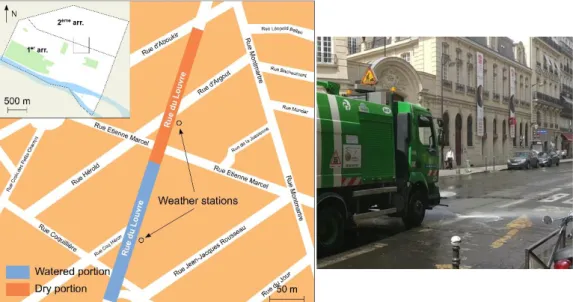
For the present case study, meteorological data was collected from two weather stations located at case and control sites under a BACI design on rue du Louvre (1st and 2nd Arrondissements) in Paris, over the summers of 2013 to 2018. Table 1 sums up the watering protocols carried out from 2013 to 2015 and from 2016 to 2018 between June and mid-September, if the criteria were met. As the pavement is shaded in the morning, the watering frequency is lower than in the afternoon while under direct insolation.
Table 1: Watering protocols carried out from 2013 to 2015 and from 2016 to 2018.
Watering protocol Portion watered Period Frequency
2013 to 2015 Road and sidewalk
(100% of the street width)
6:30 am to 12 pm 2 pm to 6:30 pm
every 1 to 2 hours every 30 minutes
2016 to 2018 Road only
(66% of the street width)
7 am to 11:30 am 2 pm to 6:30 pm
every 1.5 hours every 30 minutes Site Characteristics and Instrumentation
An illustration of the watered (case) and control portions as well as a photograph of the case weather station are provided in Figure 3. Unfortunately, from 2016 to 2018 construction work was undergoing in rue du Louvre preventing us from watering the sidewalk. Each portion is about 200 m long and 20 m wide and is equipped with a weather station in its center placed near the edge of the sidewalk. The street has a canyon aspect ratio (H/W) of approximately one and is paved with impervious asphalt concrete laid on a cement-treated base.
Figure 3: Illustration of the case and control portions in rue du Louvre (left, adapted from Hendel et al., 2016) and photograph of a cleaning truck performing watering (right).
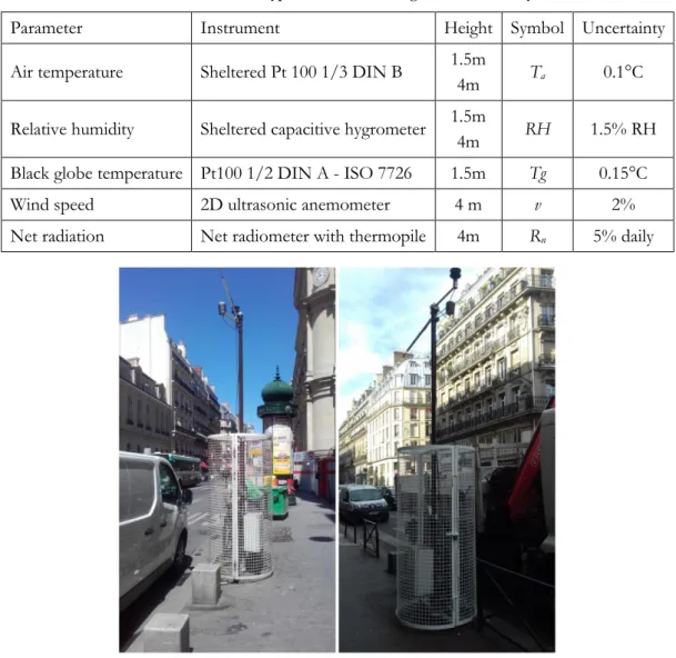
Case and control weather stations measure a number of microclimatic parameters either at pedestrian height, 4 m above ground level or both, including air temperature, relative humidity, black globe temperature, wind speed and net radiation. Instruments were placed inside white-painted cylindrical cages to prevent them from being vandalized. The net radiometer placed 4-meter height was laterally deported with a 1.5 m-metallic arm to limit the station’s cage potential impact on the measurement. All measured parameters are listed in Table 2.
Table 2: Instrument type, measurement height and uncertainty.
Parameter Instrument Height Symbol Uncertainty
Air temperature Sheltered Pt 100 1/3 DIN B 1.5m
4m Ta 0.1°C
Relative humidity Sheltered capacitive hygrometer 1.5m
4m RH 1.5% RH
Black globe temperature Pt100 1/2 DIN A - ISO 7726 1.5m Tg 0.15°C
Wind speed 2D ultrasonic anemometer 4 m v 2%
Net radiation Net radiometer with thermopile 4m Rn 5% daily
Figure 4: Photographs of the case (left) and control (right) weather stations in rue du Louvre.
Watering Criteria
Pavement-watering is conducted with a cleaning truck and manual operator if certain meteorological conditions are met, corresponding to relaxed heat-wave conditions. These conditions are based on Météo-France’s 3-day forecast for the test day. Pavement-watering criteria, as well as the heat-wave warning criteria for Paris, are summarized in Table 3.
Table 3: Weather conditions required for pavement-watering and heat wave warnings (Hendel et al. 2016)
Parameter Pavement-watering Heat-wave warning level
Ta
3-day mean of Tmin ≥ 16°C ≥ 21°C for three consecutive days
3-day mean of Tmax ≥ 25°C ≥ 31°C for three consecutive days
v ≤ 10 km/h -
Sky conditions Sunny (less than 3 oktas cloud cover) -
The sky and wind speed conditions automatically filter for days of Pasquill Stability Class A or A-B, i.e. strong to moderate solar radiation with wind speeds lower than 3 m/s (Pasquill 1961). The three-day mean condition imposed on maximum and minimum air temperature entails that observations in the days leading up to or following pavement-watering are often also of Pasquill Stability Class A or A-B. Since these days are not watered, they are used as reference observations. Furthermore, since pavement-watering is a fully reversible UHI countermeasure, reference and watered observations continue to be obtained every summer
that the weather stations continue recording and that pavement-watering is tested. Reference and countermeasure periods are thus intertwined, occurring throughout the summer.
Two families of datasets are constructed from the same measurement stations: one for the reference days and one for the watering days. Measurements were performed every minute (i.e. the total number of datasets is K = 1,440). For all the upcoming analyses, one-minute data series are smoothed with a ten-minute centered moving average as per Van der Hoven (1957) to filter out outliers and spikes caused by meteorological turbulence.
The effects on pedestrian heat stress were assessed using the Universal Thermal Climate Index (UTCI) (Blazejczyk et al. 2010). The UTCI-equivalent temperature was calculated using the fast-calculation script available online (Bröde 2009).
2. Results
We begin by presenting the results of the 2013 to 2015 campaigns for which 100% of the street width was watered.
2.1. Effects of Street and Sidewalk Watering: 2013 to 2015
During the experimental campaigns from 2013 to 2015, a total of Ncounter = 16 watering days and Nref = 28
reference days were recorded based on the criteria presented in Table 3, the vast majority of which occurred in June and July. For the linear fixed-effects approach, the relationship between interstation profiles was studied considering the implementation of the countermeasure as the fixed effect, i.e. is the pavement watered (countermeasure period) or not (reference period). To avoid compromising the statistical robustness of the method, no random effects were considered due to the lack of observations.
On the results, we will only take interest in the value of the slope of the model, which is equivalent to the impact of watering (see eq. (6)). Both the intercept (∆𝑀𝑟𝑒𝑓) and slope (𝐼) are left free (not imposed) as far as they are expected to change throughout the day. The calculation of the statistical significance is independent from the measurement frequency: for each minute, a test is performed to compare the random variables from each population (namely ∆𝑀𝑟𝑒𝑓and ∆𝑀𝑐𝑜𝑢𝑛𝑡𝑒𝑟) on the whole sample available (that is Ncounter and Nref
observations). That way, all 1,440 datasets are tested independently, each with all reference and watered observations recorded.
Figure 5 shows the results for the 2013 to 2015 campaign using the FEM model for air temperature (Ta)
and relative humidity (RH) at 1.5 m (left) and 4 m height (right), mean radiant temperature (MRT) and UTCI-equivalent temperature. Average effects are plotted as solid blue lines. 95%-confidence intervals are plotted as dashed green lines while statistically significant observations (i.e. those outside of the 95% confidence interval) are emphasized in red. A close-up of the statistically significant results is provided in Table 4.
Figure 5: Average watering effects at Louvre calculated with a linear fixed-effects model with 16 watering days and 28 reference days overs the summers of 2013, 2014 and 2015 (top to bottom) for Ta, RH at 1.5m (left) and 4m (right) above ground level and MRT (bottom left) and UTCI (bottom right). Average effects are solid blue, confidence interval with
significance interval 95% is dashed green and statistically significant events are emphasized in red.
MRT h=1.5m UTCI h=1.5m
h=4m h=1.5m
h=4m h=1.5m
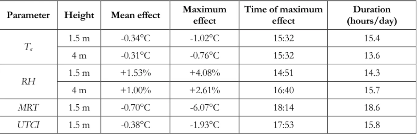
Table 4: Duration, average and maximum values and occurrence hour of maximum effect for statistically significant events of pavement watering at Louvre between 2013 and 2015 using a linear fixed-effects approach
Parameter Height Mean effect Maximum effect Time of maximum effect (hours/day) Duration
Ta 1.5 m -0.34°C -1.02°C 15:32 15.4 4 m -0.31°C -0.76°C 15:32 13.6 RH 1.5 m +1.53% +4.08% 14:51 14.3 4 m +1.00% +2.61% 16:40 15.7 MRT 1.5 m -0.70°C -6.07°C 18:14 18.6 UTCI 1.5 m -0.38°C -1.93°C 17:53 15.8
Table 4 summarizes mean and maximum statistically significant effects. The total duration of statistically significant events is used as a control parameter that quantifies the robustness of the watering effects. Although not presented here, the analysis could be further refined by averaging the effects in the morning only, or the afternoon or evening.
Compared to previous work by Hendel et al. (2016) on the assessment of the watering effects in 2013 and 2014 only, very similar results are found, especially for the mean effects and the duration of statistically significant events. The only significant exception is noted for RH for which fewer statistically significant events are identified, not because of a larger margin of error but because of a reduction of the average effects following the addition of 2015 data to the analysis, i.e. a smaller signal-to-noise ratio.
On the other hand, thanks to the additional days of the summer of 2015 and to the analysis method, maximum effects are roughly doubled for all microclimatic indicators with regard to previous analyses (Hendel et al. 2016). Globally, for Ta and RH, statistically significant events occur soon after the beginning
of watering (around 9am) and remain so until 6am the next day. Two main interruptions in the statistically significant events should be noted: approximately between 1pm and 2pm, corresponding to the interruption of watering due to operational team turnover, and the another one between 8pm and 10pm. Although the reason for the latter is unclear, even if effects are not statistically significant, average profiles are always positively affected by watering. For MRT and UTCI, most of the statistically significant events occur in the morning and the evening with fewer statistically significant effects in the afternoon because of the stronger data variability, while some statistically significant effects can even be observed at night up until the next morning.
Possibly, the latter events could be influenced by the data treatment, in case watering were to affect the suitability of the previous/following day to be used as a reference day. However, this is only true if a reference day directly precedes (leading to a cumulative watering effect) or follows (leading to an underestimation of the impact in the following morning) a watering day. Here this seems unlikely as only one reference day directly follows watering, while remaining watering and reference observations are decorrelated. The same goes for the 2016-to-2018 period with two reference days following watering. Thus, possible lagged-correlation in time should be smoothed out in the complete set of observations used in the FEM. Furthermore, night-time and next-morning effects have a particularly small amplitude (close to zero for all indicators), and as such are the only effects eliminated when setting the statistical significance to 99% instead of 95%. Their microclimatic impact therefore remains limited, although not unlikely: slight thermal effects were observed at night after watered on 5 cm deep pavement heat flux signal (Hendel et al. 2015a). In all cases, maximum effects occur during the afternoon, i.e. under direct insolation of the street. An improvement of UTCI-equivalent temperature up to -1.93°C is detected.
2.2. Effects of street-only watering: 2016 to 2018
For the 2016-2018 campaign, where only the pavement was watered, 9 watering days and 20 reference days were recorded. Results for the 2016-2018 campaign using the fixed-effects model are plotted in Figure 6 and associated results summarized in Table 5.
Figure 6: Average watering effects at Louvre calculated with a linear fixed-effects model with 9 watering days and 20 reference days overs the summers of 2016, 2017 and 2018 (top to bottom) for Ta, RH at 1.5m (left) and 4m (right) above ground level and MRT (bottom left) and UTCI (bottom right). Average effects are solid blue, confidence interval with
significance interval 95% is dashed green and statistically significant events are emphasized in red.
h=1.5m h=4m
MRT UTCI
h=1.5m h=4m
Table 5: Duration, average and maximum values and occurrence hour of maximum effect for statistically significant events of pavement watering at Louvre between 2016 and 2018 using a linear fixed-effects approach
Parameter Height Mean effect Maximum effect maximum Time of
effect Duration (hours/day)
Ta 1.5 m -0.36°C -0.97°C 13:50 7.5 4 m -0.37°C -0.81°C 13:31 10.8 RH 1.5 m +1.34% +3.03% 16:27 13.7 4 m +1.13% +2.33% 15:57 14.8 MRT 1.5 m -0.82°C -10.01°C 17:49 12.6 UTCI 1.5 m -0.46°C -3.42°C 17:49 6.0
In this configuration, similar mean and maximum effects are obtained compared to watering both road and sidewalk (Table 4), with the exception of MRT and UTCI, discussed below. The duration of statistically significant effects however is globally halved compared to the 2013-2015 campaign. For Ta, most of the
statistically significant effects are observed either in the morning or in the evening, but vanish in the afternoon, that is during the direct insolation period. This holds true for MRT as well. On the other hand,
RH is only weakly affected by the change of watering strategy both in terms of duration and mean value of
statistically significant effects, although maximum statistically significant effects are reduced by one percentage point compared to Table 4, which is, all else being equal, beneficial for thermal comfort. For both Ta and RH, the mean effect and duration of statistically significant effects are higher 4 m above
ground level than at pedestrian height. This can be interpreted as being the result of the microclimatic spatial contrast between the sidewalk (dry) and the road (wet). This contrast between the wet road and dry sidewalk is stronger 1.5 m above ground level than at a height of 4 m where the air is better mixed.
Concerning MRT, strong variability is observed in the afternoon with an important margin of error. As a result, only sporadic statistically significant effects are observed during this period. This is also true for
UTCI, although statistically significant effects are only observed in the morning for the latter while some
are also observed in the evening for MRT. As a result, compared to 2013-2015, three times fewer statistically significant effects are observed in 2016-2018 (with respective durations of the effects of 6h versus 15.8h). Also, under direct insolation, maximum effects reached for MRT seem to be unreasonably high with regard to results obtained from the 2013-2015 campaign (with maximum effects of -6.07°C versus -10.01°C here), given that results from 2016-2018 are expected to be smaller, since a smaller surface is watered. Consequently, UTCI is also affected.
From 2016 to 2018, data from only 9 watering days is available for this analysis. Combined with the strong variability in both ∆𝑀𝑟𝑒𝑓and ∆𝑀𝑐𝑜𝑢𝑛𝑡𝑒𝑟in the afternoon, especially for black globe temperature, we assume that the lower signal-to-noise ratio in 2016 to 2018 compared to that of 2013 to 2015 partly explains the results mentioned in the previous paragraph. The higher maximum effects for 2016 to 2018 could also be explained by summer 2018’s harsher-than-usual meteorology which may have increased the efficiency of watering that year. It should be noted that, 12 reference days out of 20 and 7 watering days out of 9 occurred in 2018.
3. Discussion
In both watering strategies tested, statistically significant effects were observed for each microclimatic indicator considered, resulting in a reduction of pedestrian heat stress with longer-lasting effects when watering both road and sidewalk.
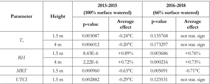
To assess the effectiveness and robustness of each strategy in greater detail, a FEM analysis can be performed on the 24-hour averaged watering effect to test for its statistical significance or not with a 95% confidence interval. Results are reported in Table 6 for each watering strategy. No average effect is presented if not statistically significant.
Table 6: p-value and associated 24-hour average statistically significant effect at Louvre for the 2013-2015 and 2016-2018 campaigns Parameter Height 2013-2015 (100% surface watered) 2016-2018 (66% surface watered) p-value Average effect p-value Average effect
Ta
1.5 m 0.003087 -0.24°C 0.135768 not stat. sign
4 m 0.006012 -0.20°C 0.173297 not stat. sign
RH 1.5 m 8.43E-6 +0.89% 0.003686 +0.76%
4 m 2.22E-6 +0.72% 0.000216 +0.73%
MRT 1.5 m 0.000960 -0.63°C 0.005091 -0.71°C
UTCI 1.5 m 0.002882 -0.29°C 0.123531 not stat. sign For 2013 to 2015, for each parameter, we denote that the p-value is much lower than 0.05, meaning that the 24-hour average effect is highly stat. sig. This was already the case for 2013-2014 (Hendel et al. 2016). Also, the p-values for 2013-2015 are systematically lower than for 2016-2018 for all parameters. For the latter campaign, the 24-hour average effect is nonetheless statistically significant for RH at both heights and for
MRT. On the other hand, no statistically significant effect is observed for Ta nor for UTCI when considering
a significance level of 0.05.
In terms of heat stress, this confirms that watering of the road and the sidewalk, i.e. 100% of the street width, is more efficient than watering only the road, i.e. about 66% of the street width for this site. Such results were already highlighted in previous work where only 33% of the pavement at Belleville site was watered compared to 100% at Louvre (Hendel et al. 2016). This is unsurprising since the cooling effects are directly linked to the watered surface area, though other factors directly influencing evaporation must be taken into account such as the ground surface temperature, air temperature, convection exchanges, vapour pressure gradient in the near air, etc.
The first limitation when comparing both watering campaigns is that the weather stations used to perform the measurements were placed on the sidewalk where pedestrians are expected to be present. As such, the stations were not in the watered area (road) from 2016 to 2018 contrary to watering conducted from 2013 to 2015. Watering only the sidewalk instead of only the road for the same watered surface area might lead to greater cooling effects than those exhibited here.
The second limitation of the comparison of both strategies is due to the fact that the number of days used to conduct the statistical analyses is much smaller for 2016-2018 than for 2013-2015 (respectively, 20 versus 28 for reference days and 9 vs 16 for watered days). For the general case, the main risk is that even though the average interstation profile is positively affected by watering, the higher variance of the measurements results in p-values greater than the significance level (thus not statistically significant). This may not necessarily be due to the less efficient strategy itself, but because of an increased standard deviation due to the smaller sample size. This compounds with the fact that the expected effects of a reduced watering strategy are particularly small and decrease the signal-to-noise ratio, requiring a larger number of measurements to compensate for this. In a nutshell, ideally, different strategies should be compared under the same conditions. Here, this means using the exact same number of days in the analysis for each campaign. This is necessary to obtain identical noise and thus properly isolate the exact impact of each strategy. However, this does not affect the average effects found here. Again, the best way to overcome this problem is to increase the sample size.
In the case of our experiment, acquiring more data can be complicated since it is quite time-consuming (several summers in Paris given the weather criteria that were set) and operationally-intense, combined with the fact that weather station failures reduce the number of observations further. Also, the use of a greater number of days acquired on a large time span should be carefully performed in a BACI experiment and is only relevant provided that the difference between stations either remains constant or depends on known factors that can be accounted for in a LMM.
Future avenues for improvement of the analysis concern this point, i.e. taking into account relevant random factors to apply a proper LMM, which requires a larger statistical sample to be relevant. In its current state, the FEM assesses a global impact of the countermeasure on the whole set of observations, regardless of potential intra-correlations between datasets caused by random factors (weather or insolation conditions, summer period, etc.). These must be investigated to incorporate their influence on the gathered data. Finally, alternative Bayesian or machine learning approaches as alternative statistical tools could also be useful for further improvements of the method.
Conclusion
A methodology for assessing the effects of UHI-countermeasure in the field was proposed by adapting the Lowry approach. The framework identified that the performance of UHI countermeasures cannot be evaluated in the field with direct comparisons between case and control observations as these do not eliminate pre-existing interstation differences. To evaluate their performance, the difference between reference (before) and countermeasure (after) measurements must be tested under the BACI design. Furthermore, it was also shown that countermeasure and reference observations cannot be considered independent and the statistical tools used to test their statistical significance must account for this. A statistical methodology was proposed to evaluate the cooling performance of pavement-watering conducted at rue du Louvre in Paris from 2013 to 2018. The methodology can be generalized to other UHI countermeasures, provided that microclimatic measurements start sufficiently ahead of the implementation of the countermeasure put in place.
For the linear fixed-effects model, the interstation difference for each parameter was expressed as a function of fixed effects, i.e. before or after implementation of the countermeasure. Unfortunately, the total number of observations was too small to conduct a robust linear mixed model analysis, taking into account relevant random factors. A fixed-effect model was therefore used in place of a LMM. This approach does not require data pairing and can therefore be used with asymmetric sample datasets, making it much simpler to implement in the general case.
From 2013 to 2015, the whole street width was watered (pavement and sidewalk). Results showed that watering days were cooler and more humid than reference days and is effective for reducing heat stress as perceived by pedestrians. In particular, watering effects reached maximum values up to -1.02°C and -0.76°C for 1.5 and 4 m air temperature respectively, +4.08% and +2.61% for 1.5 and 4 m relative humidity, and -6.07°C and -1.93°C for 1.5 m MRT and UTCI-equivalent temperature. These effects are slightly greater than those found for previous analyses performed from 2013 to 2014 using an ill-suited two-sample t-test. This is most likely thanks to the addition of the days of summer 2015 for which particularly hot conditions were experienced during all summer. Indeed, the analysis of the watering effects of only 2015 at Louvre exhibited even greater cooling effects, with reductions up to -2.84°C and average reduction of -1.16°C for 1.5 m air temperature. From 2013 to 2015, daily average effects of -0.34°C and -0.31°C for 1.5 m and 4 m air temperature, +1.53% and +1.00% for 1.5 and 4 m relative humidity, -0.70°C and -0.38°C for 1.5 m MRT and UTCI-equivalent temperature. Such effects were observed all day almost as soon as watering begins, with less robust marginal effects lasting until 6 am the next day. Fewer but stronger statistically significant effects are observed in the afternoon in general. While watering only represents a 9-hour intervention per day, its effects can be felt for about 15 hours.
From 2016 to 2018, only 66% of the street width was watered (pavement only). Unsurprisingly, this strategy was found to be less efficient than the previous though similar effects were observed. Of interest, a significant decrease of the duration of statistically significant effects was found, i.e. two or three times shorter depending on the parameter. The duration of statistically significant relative humidity effects is the least affected and UTCI-equivalent temperature the most. Statistically significant effects mainly occurred in the morning, apart for relative humidity, when the area is shaded.
The methodology will be tested further on other sites with different UHI countermeasures to provide additional information about its relevance. Such projects include the use of alternative pavements, currently being prepared by the City of Paris (Life Cool & Low Noise 2017), or the conversion of a parking lot from a dark mineral environment to a green space with permeable pavement (Parison et al. 2018). As previously stated, proper monitoring ahead of UHI countermeasure implementation is crucial in order for the method
to be robust, i.e. requiring at least 10-30 reference and countermeasure observations (i.e. measured data sampled from a given statistical population).
The method is based on a BACI design, it therefore inherits its limitations. For instance, in ever changing urban environments, an intervention lasting over several years may be subject to data drifting due to long term or periodic effects, potentially making the earliest and latest observation periods incomparable. Also, in the case where control and case sites x1 and x2 are close enough to both be affected by the UHI
countermeasure, the BACI contrast will likely be reduced, thus leading to an underestimation of the countermeasure effects. In the literature, those issues are pinpointed as the main limitations of the simple BACI design (Smith 2014). Possibilities for improvement mainly concern the implementation of a multiple BACI design (MBACI), involving a network of control stations spread across the direct vicinity of the case station (Downes et al. 2002). This limits the problem of poorly-matched sites and improves the reliability of the analysis.
For the general case, provided that enough data is available, the impact of the expected causes of long-term or periodic data drifting can be isolated by adding a corresponding random effect in a LMM. In the case of strong dependence to these effects, it is expected that the margin of error of the test would be narrowed. In either case, correlation of the datasets to random effects will be even weaker provided that case and control stations are carefully paired and that analysis days are filtered using given criteria, for example such that shading patterns change in a similar fashion. Otherwise, the effects of the countermeasure may not be properly isolated. The criteria that is chosen will most likely help filter large, local and long-lasting random effects.
Acknowledgments
Funding for this study was provided by the Waste and Water and Roads and Traffic Divisions of the City of Paris.
References
Akbari, Hashem, Melvin Pomerantz, and Haider Taha. "Cool surfaces and shade trees to reduce energy use and improve air quality in urban areas." Solar energy 70.3 (2001): 295-310.
Bernstein, Brock B., and James Zalinski. "An optimum sampling design and power tests for environmental biologists." Journal of Environmental Management 16.1 (1983): 35-43.
Błażejczyk, Krzysztof, et al. "Principles of the new Universal Thermal Climate Index (UTCI) and its application to bioclimatic research in European scale." Miscellanea Geographica 14.1 (2010): 91-102.
Bröde, Peter. "UTCI Fast Calculation Script." Documents Available Online (2009): (accessed: february 2020).
Bolker, Benjamin M., et al. "Generalized linear mixed models: a practical guide for ecology and evolution." Trends in
ecology & evolution 24.3 (2009): 127-135.
Chaves, Luis Fernando. "An entomologist guide to demystify pseudoreplication: data analysis of field studies with design constraints." Journal of medical entomology 47.3 (2010): 291-298.
Conner, Mary M., et al. "Evaluating impacts using a BACI design, ratios, and a Bayesian approach with a focus on restoration." Environmental monitoring and assessment188.10 (2016): 555.
Conquest, Loveday L. "Analysis and interpretation of ecological field data using BACI designs: discussion." Journal of
Agricultural, Biological, and Environmental Statistics (2000): 293-296.
Downes, Barbara J., et al. Monitoring ecological impacts: concepts and practice in flowing waters. Cambridge University Press, (2002).
Hendel, Martin, et al. "Improving a pavement-watering method on the basis of pavement surface temperature measurements." Urban Climate 10 (2014): 189-200.a
Hendel, Martin, et al. "An analysis of pavement heat flux to optimize the water efficiency of a pavement-watering method." Applied thermal engineering 78 (2015a): 658-669.
Hendel, Martin, and Laurent Royon. "The effect of pavement-watering on subsurface pavement temperatures." Urban
Climate 14 (2015b): 650-654.
Hendel, Martin, et al. "Measuring the effects of urban heat island mitigation techniques in the field: Application to the case of pavement-watering in Paris." Urban Climate 16 (2016): 43-58.
Himeno, S., et al. "Using Snow Melting Pipes to Verify the Water Sprinkling s Effect over a Wide Area." NOVATECH 2010 (2010).
Hoelscher, Marie-Therese, et al. "Quantifying cooling effects of facade greening: Shading, transpiration and insulation." Energy and Buildings 114 (2016): 283-290.
Hurlbert, Stuart H. "Pseudoreplication and the design of ecological field experiments." Ecological monographs 54.2 (1984): 187-211.
Kinouchi, Tsuyoshi, et al. "An observation of the climatic effect of watering on paved roads." Journal of hydroscience and
hydraulic engineering 15.1 (1997): 55-64.
Kyriakodis, G. E., and M. Santamouris. "Using reflective pavements to mitigate urban heat island in warm climates-Results from a large scale urban mitigation project." Urban Climate 24 (2018): 326-339.
Life Cool & Low Noise Asphalt Project official website (Juily 2017): https://www.life-asphalt.eu/
Loughin, Tom M., Stephen Nicholas Bennett, and Nicolaas W. Bouwes. "A comparison of asymmetric before-after control impact (aBACI) and staircase experimental designs for testing the effectiveness of stream restoration." BioRxiv (2018): 359406.
Lowry, William P. "Empirical estimation of urban effects on climate: a problem analysis." Journal of Applied
Meteorology16.2 (1977): 129-135.
Météo France and CSTB, “EPICEA Project - Final Report,” Paris, France (in French), (2012).
Millar, Russell B., and Marti J. Anderson. "Remedies for pseudoreplication." Fisheries Research 70.2-3 (2004): 397-407. Parison, Sophie, et al. "“Tierce Forêt”: Measuring the Cooling Effects from Greening a Parking Lot." in in ICUC10
& 14th Symposium on Urban Environment, (2018)
Pasquill, Frank. "The estimation of the dispersion of windborne material." Met. Mag. 90 (1961): 33.
Rosado, P., et al. "Cool pavement demonstration and study." Third International Conference on Countermeasures to Urban
Heat Island. (2014).
Smith, Eric P. "BACI design." Wiley StatsRef: Statistics Reference Online (2014).
Spronken-Smith, R. A., and T. R. Oke. "Scale modelling of nocturnal cooling in urban parks." Boundary-Layer
Meteorology93.2 (1999): 287-312.
Stewart-Oaten, Allan, William W. Murdoch, and Keith R. Parker. "Environmental impact assessment:" Pseudoreplication" in time?." Ecology 67.4 (1986): 929-940.
Tsin, Pak Keung, et al. "Microscale mobile monitoring of urban air temperature." Urban Climate 18 (2016): 58-72. Van der Hoven, Isaac. "Power spectrum of horizontal wind speed in the frequency range from 0.0007 to 900 cycles
per hour." Journal of meteorology 14.2 (1957): 160-164.
Wong, Nyuk Hien, and Chen Yu. "Study of green areas and urban heat island in a tropical city." Habitat international 29.3 (2005): 547-558.
Yamagata, H., et al. "Heat island mitigation using water retentive pavement sprinkled with reclaimed wastewater." Water science and technology 57.5 (2008): 763-771.