University of Neuchâtel
Centre for Hydrogeology
Faculty of Science
and Geothermics
Ph.D. Thesis
Riverbank Filtration
within the Context of
River Restoration and Climate Change
presented to the Faculty of Science of the University of Neuchâtel to satisfy
the requirements of the degree of Doctor of Philosophy in Science
by
Samuel Diem
Thesis defense date: 20.08.2013 Public presentation date: 19.09.2013
Ph.D. Thesis evaluation committee:
Prof. Dr. Daniel Hunkeler, University of Neuchâtel (Director of the thesis) Prof. Dr. Mario Schirmer, University of Neuchâtel (Co-director of the thesis) Prof. Dr. Philippe Renard, University of Neuchâtel
Acknowledgments
The completion of this Ph.D. Thesis would not have been possible without the support of colleagues, friends and family.
I would like to start by thanking my supervisor, Mario Schirmer. He gave me the opportunity to write this Ph.D. Thesis, supported me in any situation, had always time for discussions, provided helpful inputs, and never refused a request (course, conference, field equipment,…). I am grateful to Daniel Hunkeler for the possibility to do my Ph.D. at the CHYN and for many helpful discussions. I thank John Molson for his commitment as external examiner. I further would like to thank Philippe Renard and Olaf Cirpka who supported me with substantial ideas and instructive discussions. I am also thankful to Eduard Hoehn and Daniel Käser for their advice in various situations and stages of my Ph.D. and for motivating me in times of local and global minima in my motivation space.
Many thanks to the RIBACLIM-Team: Urs von Gunten for leading and initiating the project and for many fruitful discussions; Matthias Rudolf von Rohr for his continuous support in the field, his introduction to lab work and his optimism; Sabrina Bahnmüller for her help in the lab and the field and for always reminding me that we are all in the same boat; Janet Hering, Hans-Peter Kohler and Silvio Canonica for their uncomplicated exchange and their collaboration.
A big THANK YOU to the Hydrogeology Group (Anne-Marie, Ben, Dirk, Jana, Mehdi, Stefano, Vidhya), my office mates (Ryan, Sabine, Stephan) and the RoKi Group (Lars, Lina, Matthias, Simon, Yama). You all contributed to this thesis in some way and created an enjoyable working environment at Eawag. I thank Lena Froyland (Master student) and Roger Mégroz (Intern) for the opportunity to supervise their work. I also thank the Eawag-Werkstatt (Andy, Peter, Richi) for their technical support in the field, the Aua-Lab for analyzing all the samples, as well as the IT- and Empfang-Team for their excellent service.
Many thanks to all my friends; you helped me to release and re-adjust my mind. Finally, I would like to thank my family, especially my parents, my famous four sisters and my parents-/brother-/sisters-in-law, who always supported and encouraged me. Last but certainly not least, I would like to thank Murielle, my beloved wife. She was my backbone, supportive and understanding through it all – she showed me true love.
Abstract
Drinking water derived by riverbank filtration is generally of high quality and is an important source of drinking water in several European countries. In the future however, riverbank-filtration systems will face two major challenges – river restoration and climate change. The goal of this Ph.D. Thesis was to deepen the understanding of physical and biogeochemical processes that occur during riverbank filtration and develop new tools in order to facilitate the assessment of potential adverse effects of river restoration and climate change on the quality of river-recharged groundwater.
River restoration measures can lead to shorter residence times between the river and the pumping well and therefore can increase the risk of drinking water contamination by bacteria or pollutants. Numerical groundwater models provide quantitative information on groundwater flow paths and residence times, but require a rigorous definition of the spatial and temporal river water level distribution. In this thesis, two new interpolation methods were developed to generate time-varying 1D and 2D river water level distributions. The methods were implemented at the partly restored Niederneunforn field site at the peri-alpine Thur River (NE-Switzerland), and were applied to a 3D groundwater flow and transport model. The results confirmed the method’s suitability for accurately simulating groundwater flow paths and residence times.
The increased occurrence of heat waves due to climate change likely favors the development of anoxic conditions in the infiltration zone, which may significantly deteriorate the quality of river-recharged groundwater. Results from field sampling campaigns and column experiments suggest that particulate organic matter (POM) degradation mainly accounted for the variability of dissolved oxygen (DO) consumption during riverbank filtration. Furthermore, DO consumption was found to positively correlate with temperature and discharge. The latter was attributed to an enhanced trapping of POM within the riverbed during high-discharge conditions. To quantify the temperature and discharge dependence of DO consumption during riverbank filtration, a new semi-analytical model was developed and successfully applied to the Niederneunforn field site. The modeling approach can be transferred to other riverbank-filtration systems to efficiently estimate groundwater DO concentrations under various climatic and hydrologic conditions and, hence, to assess the risk of arising anoxic conditions.
Kurzfassung
Mittels Uferfiltration gewonnenes Trinkwasser ist generell von hoher Qualität und stellt eine wichtige Trinkwasserressource für mehrere europäische Länder dar. In der Zukunft werden Uferfiltrationssysteme jedoch mit zwei bedeutenden Herausforderungen konfrontiert – Flussrevitalisierung und Klimaänderung. Das Ziel dieser Doktorarbeit war es, das Verständnis physikalischer und biogeochemischer Prozesse während der Flussinfiltration zu vertiefen und Instrumente zu entwickeln, um potentielle negative Auswirkungen von Flussrevitalisierung und Klimaänderung auf die Qualität des Uferfiltrats besser zu erfassen.
Massnahmen der Flussrevitalisierung können zu verkürzten Fliesszeiten zwischen Fluss und Trinkwasserfassung führen, was das Risiko einer Trinkwasserkontamination mit Bakterien und Schadstoffen erhöhen kann. Numerische Grundwassermodelle liefern quantitative Informationen über Grundwasserfliesspfade und Fliesszeiten, benötigen aber eine genaue Definition der räumlichen und zeitlichen Flusswasserstandsverteilung. In dieser Arbeit wurden zwei neue Interpolationsmethoden entwickelt, um zeitlich variable 1D und 2D Flusswasserstandsverteilungen zu generieren. Die Methoden wurden am teilweise revitalisierten Feldstandort Niederneunforn am voralpinen Fluss Thur (Nordostschweiz) implementiert und auf ein 3D Grundwasserströmungs- und Transportmodell angewandt. Die Resultate bestätigten die Eignung der Methoden zur präzisen Simulation von Grundwasserfliesspfaden und Fliesszeiten.
Das vermehrte Auftreten von Hitzewellen aufgrund der Klimaänderung begünstigt möglicherweise die Ausbildung anoxischer Verhältnisse in der Infiltrationszone, was die Qualität des Uferfiltrats deutlich verschlechtern würde. Die Resultate aus Feldprobennahmen und Säulenversuchen deuten darauf hin, dass der Abbau von partikulärem organischem Material (POM) hauptsächlich für die Variabilität der Sauerstoffzehrung während der Flussinfiltration verantwortlich war. Zusätzlich wurde eine positive Korrelation zwischen der Sauerstoffzehrung und der Temperatur sowie dem Abfluss festgestellt. Letztere wurde einem erhöhten Eintrag von POM in das Flussbett während Hochwasserbedingungen zugeschrieben. Um die Temperatur- und Abflussabhängigkeit der Sauerstoffzehrung während der Flussinfiltration zu quantifizieren, wurde ein neues semi-analytisches Modell entwickelt und erfolgreich am Feldstandort Niederneunforn angewandt. Der Modellansatz lässt sich auf weitere Uferfiltrationssysteme übertragen, um Sauerstoffkonzentrationen im Grundwasser effizient abzuschätzen, und somit das Risiko aufkommender anoxischer Bedingungen zu beurteilen.
Résumé
L’eau de consommation provenant de la filtration sur berge est généralement de bonne qualité et constitue une source d’eau potable dans plusieurs pays de l’Union Européenne. A l’avenir pourtant, la filtration sur berge devra faire face à deux défis majeurs: les programmes de restauration de rivière et les changements climatiques. La présente thèse vise, d’une part, à approfondir la compréhension des processus physiques et biogéochimiques liés à la filtration sur berge et, d’autre part, à développer de nouveaux outils pour évaluer les impacts potentiels des programmes de restauration et des changements climatiques sur la qualité de l’eau souterraine provenant de ces techniques de filtration.
Les mesures de restauration de rivière peuvent conduire à un raccourcissement des temps de résidence de l’eau entre la rivière et le puits de pompage, et ainsi augmenter les risques de contamination chimique et microbiologique. La modélisation hydrodynamique est une approche quantitative privilégiée pour identifier les chemins d’écoulements souterrains et quantifier les temps de résidence; elle requiert cependant une définition rigoureuse de la variabilité spatiale et temporelle des niveaux de rivière. Dans cette thèse, deux méthodes d’interpolation sont développées pour générer une représentation temporelle adéquate des niveaux de rivières en 1D et 2D. Ces méthodes sont testées sur le site expérimental et partiellement restauré de Niederneunforn (NE de la Suisse), situé sur la rivière préalpine Thur, et sont implémentées dans un modèle numérique d’écoulement et de transport souterrain 3D. Les résultats confirment la pertinence de ces méthodes pour la simulation précise des chemins d’écoulements et des temps de résidence.
Avec les changements climatiques, l’augmentation de la fréquence des vagues de chaleur favorisera probablement le développement de conditions anoxiques dans les zones d’infiltration de la rivière, ce qui tendra à détériorer la qualité de l’eau souterraine rechargée par filtration de berge. Les résultats de campagnes d’échantillonnage et d’expériences sur colonne suggèrent que la dégradation de la matière organique particulaire (MOP) est la principale cause de variabilité de la consommation en oxygène dissous (OD) liée au processus de filtration sur berge. En outre, la consommation de l’OD apparaît positivement corrélée à la température et au débit de la rivière. Cette seconde corrélation est attribuée au piégeage accru de la MOP dans le lit du cours d’eau pendant les périodes de hauts débits. Finalement, afin de quantifier l’influence de la température et du débit sur la consommation en OD dans un contexte de filtration sur berge, un modèle semi-analytique original est développé et évalué, avec succès, sur les données du site de Niederneunforn. Cette approche de modélisation est
transférable à d’autres sites de filtration sur berge où des outils performants sont nécessaires pour estimer les teneurs en OD dans diverses conditions climatiques et hydrologiques, et évaluer ainsi le risque de développement de conditions anoxiques.
Keywords
Riverbank filtration; river restoration; climate change; groundwater flow and reactive transport modeling; stochastic-convective reactive transport; river water level distribution; particulate organic matter; oxygen consumption
Stichwörter
Uferfiltration; Flussrevitalisierung; Klimaänderung; Grundwasserströmungs- und reaktive Transportmodellierung; stochastisch-konvektiver reaktiver Transport; Flusswasserstands-verteilung; partikuläres organisches Material; Sauerstoffzehrung
Mots clés
Filtration sur berge; restauration de rivière; changements climatiques; modélisation numérique d’écoulement et de transport souterrain; transport stochastique-convectif réactif; distribution des niveaux de rivière; matière organique particulaire; consommation en oxygène dissous
Content
Chapter 1 Introduction ... 1
1.1 Motivation and background ... 1
1.2 Objectives and structure of this thesis ... 8
Chapter 2 New methods to estimate 2D water level distributions of dynamic rivers ... 11
2.1 Introduction ... 12
2.2 Interpolation methods to estimate river water levels ... 13
2.3 Application to the Niederneunforn field site ... 17
2.4 Discussion ... 22
2.5 Conclusions ... 23
2.6 Supporting information ... 25
Chapter 3 Assessing the effect of different river water level interpolation schemes on modeled groundwater residence times ... 37
3.1 Introduction ... 38
3.2 Interpolation methods ... 39
3.3 Method implementation ... 41
3.4 Groundwater flow and transport model ... 47
3.5 Results and discussion ... 51
3.6 Conclusions ... 58
3.7 Supporting information ... 61
Chapter 4 NOM degradation during river infiltration: Effects of the climate variables temperature and discharge ... 65
4.1 Introduction ... 66
4.2 Materials and methods ... 68
4.3 Results and discussion ... 73
4.5 Supporting information ... 86
Chapter 5 Modeling the dynamics of oxygen consumption during riverbank filtration by a stochastic-convective approach ... 89
5.1 Introduction ... 90
5.2 Theory ... 92
5.3 Materials and methods ... 95
5.4 Results and discussion ... 99
5.5 Conclusions ... 111
Chapter 6 Conclusions and Outlook ... 115
6.1 Conclusions ... 115
6.2 Outlook ... 120
Chapter 1
Introduction
1.1 Motivation and background
Riverbank filtration provides an inexpensive, sustainable and yet effective means to improve the quality of surface water (Tufenkji et al., 2002). During passage through the riverbed and the aquifer, the infiltrated river water is exposed to processes like sorption, physicochemical filtration and biodegradation. These natural attenuation processes efficiently remove suspended particles, bacteria, viruses, parasites, micropollutants, and other organic and inorganic compounds usually present in surface waters, such as natural organic matter and ammonium (Kuehn and Mueller, 2000; Sacher and Brauch, 2002). The effectiveness of riverbank filtration has long been recognized in Europe, where several countries cover considerable fractions of their drinking water demand by riverbank filtration (~50% in France and Slovak Republic, ~48% in Finland, ~45% in Hungary, ~25% in Switzerland and ~16% in Germany (Hiscock and Grischek, 2002; Tufenkji et al., 2002)). Hence, riverbank filtration provides an important drinking water resource, which needs to be maintained and protected, especially within the context of upcoming challenges such as river restoration and climate change. Even though experience of more than a century in the operation of riverbank-filtration systems exists, the current understanding of bank-riverbank-filtration schemes is primarily based on empirical knowledge (Hiscock and Grischek, 2002). Therefore, the adequate management of riverbank-filtration systems in a changing environment requires a better understanding of the physical and biogeochemical processes that occur during riverbank filtration (Hoehn and Meylan, 2009), which is the motivation for this Ph.D. Thesis.
1.1.1 Riverbank filtration
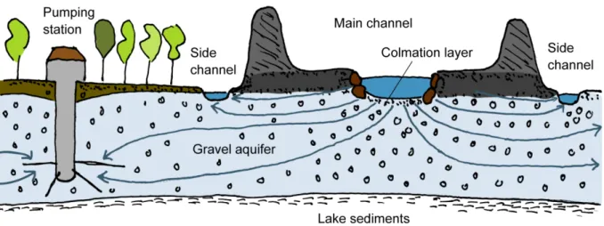
Riverbank filtration can occur under natural conditions or can be induced by a lowering of the groundwater table below surface water levels either by hydraulic boundaries such as side channels, or by groundwater abstraction at pumping wells (Fig. 1.1). Infiltration occurs mostly under saturated conditions, in direct hydraulic connection to the groundwater table (Hiscock and Grischek, 2002). If the groundwater table is more than a few decimeters below the riverbed, the hydraulic connection is lost and river water infiltrates through an unsaturated zone, which is aerated (Brunner et al., 2009; Hoehn and Meylan, 2009). Riverbank-filtration systems are typically positioned in alluvial valley aquifers, which predominantly consist of
gravels and sands allowing for high abstraction rates. However, floodplain deposits are complex geologic systems that exhibit heterogeneity on different scales and can include highly conductive “open framework gravels” forming preferential groundwater flow paths, as well as layers of silt and clay (Huggenberger et al., 1998).
Besides the dilution of the freshly infiltrated river water with ambient groundwater at the pumping well, the residence time of the bank filtrate has been identified as one of the key factors determining the removal efficiency of riverbank filtration. Several studies have shown that concentrations of natural organic matter and organic contaminants decreased with increasing travel time (Sontheimer, 1980; Grünheid et al., 2005). Also, the removal of pathogenic microbes was found to be strongly related to the residence time. A breakthrough of E. Coli at a pumping station at the Rhine River was observed after a flood event, due to shortened groundwater residence times (Eckert and Irmscher, 2006). Therefore, to ensure an adequate quality of produced water, minimal residence times are often required by law and are regulated via the definition of protection zones (FOEN, 2012b). The required minimal groundwater residence time between the river and a pumping well is 10 d in Switzerland (BUWAL, 2004) and 50 d in Germany (DVGW, 2000).
Infiltrating river water is subject to strong geochemical changes that are related to redox reactions, dissolution/precipitation of minerals, ion exchange and gas exchange (Jacobs et al., 1988; Tufenkji et al., 2002). Numerous studies have demonstrated that the most significant geochemical changes were associated with the biodegradation of natural organic matter (Jacobs et al., 1988; Bourg and Bertin, 1993; Brugger et al., 2001b; Sobczak and Findlay, 2002; Tufenkji et al., 2002). These degradation reactions were found to occur dominantly within the first meters of infiltration, where the microbial abundance and activity was highest (von Gunten et al., 1994; Brugger et al., 2001a). This interface between the river and alluvial groundwater, the hyporheic zone, has been identified as a distinct environment playing a crucial functional role in the biogeochemical cycling of nutrients and organic matter (Brunke and Gonser, 1997; Boulton, 2007).
Natural organic matter (NOM) in river systems originates from both allochthonous (terrestrially-derived) sources and generally more biodegradable autochthonous sources (periphyton) (Pusch et al., 1998; Leenheer and Croue, 2003). NOM is composed of dissolved organic matter (DOM) and particulate organic matter (POM). During infiltration of river water, DOM is transported through the riverbed as a “mobile substrate”, whereas POM is retained in the riverbed sediments as a “stationary substrate” (Pusch et al., 1998). The
retention and storage of POM within the riverbed was found to depend on the grain-size distribution of the riverbed sediments and the hydrologic conditions (Brunke and Gonser, 1997).
The microbial degradation of NOM in riverbed sediments leads to a consumption of dissolved or solid terminal electron acceptors such as oxygen (O2), nitrate (NO3-) and
Mn(III/IV)-/Fe(III)(hydr)oxides. In case of oxygen depletion, the redox sequence proceeds to denitrification followed by reductive dissolution of manganese and ferric oxyhydroxides releasing dissolved Mn(II) and Fe(II). These species are undesired and need to be removed from pumped water by additional cost-intensive treatment steps (Kuehn and Mueller, 2000). Furthermore, re-oxidation of dissolved Mn(II) and Fe(II) when mixing with aerobic water at the pumping well can cause clogging of the well screen. It also has been recognized that redox conditions can significantly influence the removal efficiency of riverbank filtration. The degradation of DOM and several organic micropollutants was found to be less effective under anoxic conditions (Schwarzenbach et al., 1983; Grünheid et al., 2005; Massmann et al., 2006; Maeng et al., 2010).
The temperature dependence of the microbially mediated NOM degradation is well known (O'Connell, 1990; Kirschbaum, 1995). As a result, redox conditions at various bank-filtration systems were observed to undergo seasonal variations with the occurrence of anoxic conditions in summer (von Gunten et al., 1991; Greskowiak et al., 2006; Massmann et al., 2006; Massmann et al., 2008). Besides temperature, the redox conditions in the infiltration zone are also influenced by the availability of electron donors (NOM, ammonium) and electron acceptors (dissolved oxygen, nitrate). During industrialization in the 1950s and 1960s, rivers in urban catchments carried higher loads of organic substances and ammonium (Eckert and Irmscher, 2006). Combined with lower oxygen concentrations in river water, strongly reducing conditions prevailed in the infiltration zones of many riverbank-filtration systems, which caused the mobilization of manganese and iron. Since the 1970s, river water quality has improved significantly and oxic conditions in infiltration zones re-established (Kuehn and Mueller, 2000).
The retention of fine suspended particles (<2 mm) during riverbank filtration contributes to the clogging of the riverbed and the development of a colmation layer (Fig. 1.1), which is characterized by a reduced permeability causing lower infiltration rates and higher residence times of infiltrated river water (Brunke, 1999). The colmation layer may be subject to strong spatial heterogeneity and temporal variability. Bed-moving floods can rework the riverbed
and cause a decolmation with an inherent increase in riverbed permeability (Schubert, 2002; Doppler et al., 2007). The higher permeability during floods was found to promote the import of POM into gravelly riverbed sediments, which in turn enhanced the microbial respiration rate (Naegeli et al., 1995). The colmation of the riverbed can have a positive effect on the removal of organic and inorganic pollutants and bacteria due to higher residence times (Hiscock and Grischek, 2002). On the other hand, a colmation layer may adversely affect groundwater quality, as higher residence times also favor the development of anoxic conditions and the mobilization of Mn(II) and Fe(II) (Tufenkji et al., 2002).
Fig. 1.1. Schematic illustration of riverbank filtration. Infiltrated river water passes the riverbed and the aquifer and is extracted at a pumping station, where it mixes with ambient groundwater and may undergo secondary treatment steps before being supplied to the drinking water distribution system. Adapted from Schirmer (2013).
1.1.2 Challenge 1: River restoration
Over the past few decades, there has been a shift in perspective of water authorities from river corridor channelization toward restoration. As a consequence, several laws have been established such as the European Water Framework Directive (European-Commission, 2000) or the Swiss Water Protection Law (GSchG, 2011; GSchV, 2011) that require engineering tasks in river courses to jointly improve flood protection, ecological status and water quality. In Switzerland, 15000 km of river length are strongly engineered, channelized and in a bad ecological condition, of which 4000 km will undergo river restoration during the next 80 years (FOEN, 2012c).
River restoration measures may comprise removal of the bank stabilization and the colmation layer, widening of the riverbed, as well as the establishment of braided river sections, re-meandering stream reaches and gravel bars (Fig. 1.2). These actions enhance the exchange between the river and the hyporheic zone and increase the habitat diversity, both being essential for the ecological health of a river system (Brunke and Gonser, 1997; Baumann et al., 2009). The higher exchange with the hyporheic zone is thought to increase the interstitial microbial activity and therefore the removal of various contaminants. However, the widening of the riverbed and the higher riverbed permeability might decrease groundwater residence times and therewith increase the risk of drinking water contamination by pollutants or bacteria (Hoehn and Scholtis, 2011). Due to a lack of process understanding and following the precautionary principle, river restoration measures are not allowed within the protection zones of drinking water wells (FOEN, 2012b).
To mitigate this conflict of interest between river restoration and drinking water protection, a good knowledge of the physical and biogeochemical processes is needed. More specifically, the well-capture zone, groundwater flow paths, flow velocities, groundwater residence times and the fraction of freshly infiltrated river water need to be known (Hoehn and Meylan, 2009). Several methods based on natural tracers such as temperature and electrical conductivity were developed to quantify exchange rates (Anderson, 2005; Kalbus et al., 2006; Vogt et al., 2010b), travel times and the fraction of riverbank filtrate in abstracted water (Hoehn and Cirpka, 2006; Cirpka et al., 2007; Vogt et al., 2010a). However, these methods are not able to provide information on groundwater flow paths and flow velocities. To this end, groundwater flow and transport modeling is a powerful tool, as it provides a quantitative link between groundwater residence times, flow paths and flow velocities (Wondzell et al., 2009).
It is well known from modeling studies and field observations that riverbed morphology affects the river water level distribution, which in turn affects or drives the exchange with groundwater (Harvey and Bencala, 1993; Woessner, 2000; Cardenas et al., 2004; Cardenas, 2009; Käser et al., 2009). Accordingly, one of the prerequisites for the setup of a groundwater flow model of a real river-groundwater system is an accurate description of the water level distribution in the river (Käser et al., 2013). However, restored river systems may have complex water level distributions that need to be characterized by their full spatial (i.e. two horizontal dimensions) and temporal extent (i.e. for any discharge condition). Ideally, such water level information is extracted from hydraulic models (Doppler et al., 2007; Derx et al., 2010; Engeler et al., 2011), but their setup is time consuming and requires a considerable amount of data input, that is, the riverbed’s bathymetry and water level information for the
calibration and validation process. Therefore, there is a need for alternative methods to describe surface water level distributions of dynamic rivers that allow for reliable simulations of the groundwater flow field and accurate predictions of groundwater residence times. Additionally, the sensitivity of these predictions on the method selection and the level of detail in the water level distribution related to these methods should be assessed.
Fig. 1.2. Schematic illustration of a restored riverbank-filtration system. The riverbed was widened, the colmation layer removed and gravel bars were established. These river restoration measures promote hyporheic exchange (orange arrows) and the development of new habitats. On the other hand, flow paths between the river and the pumping well may be shortened, which can cause a contamination of the drinking water by pollutants or bacteria. Beaver dams in side channels can lead to higher water levels that may reverse the hydraulic gradient. Adapted from Schirmer (2013).
1.1.3 Challenge 2: Climate change
Today, most peri-alpine alluvial gravel-and-sand aquifers are oxic owing to the low loads of organic matter and nutrients in rivers. Oxic conditions allow a beneficial minimal treatment of pumped groundwater before supplying it as drinking water to the distribution system. However, during the hot summer of 2003, which was accompanied by low river discharges and river temperatures of more than 25°C (OcCC, 2005), the redox conditions in numerous riverbank-filtration systems turned anoxic over a period of up to three months (Eckert et al., 2008) and the onset of denitrification was observed (Sharma et al., 2012). Denitrification may result in elevated concentrations of nitrite (NO2-), which is of concern due to its toxicity.
Hoehn and Scholtis (2011) even reported a case where the redox sequence proceeded to Mn(IV)- and Fe(III)-reducing conditions. As mentioned in Section 1.1.1, the appearance of dissolved Mn(II) and Fe(II) in the abstracted water requires additional treatment processes, and precipitation of Mn(IV)-/Fe(III)(hydr)oxides can lead to clogging of the filter screen.
Furthermore, compounds that are better degraded under oxic conditions such as DOM, ammonium and certain micropollutants are more persistent under anoxic conditions and may appear at the pumping well in elevated concentrations (Section 1.1.1).
For Europe, climate models predict an increase in air temperature, a decrease in summer rainfall and an increase in winter rainfall, as well as an increased frequency and intensity of weather extremes such as heat waves or flood events (IPCC, 2007), which is consistent with the climate-change scenarios for Switzerland (CH2011, 2011). River discharges are expected to decrease in summer and increase in winter. River water temperature, which is decisive for the degradation processes within the riverbed, is likely to increase by the same extent as air temperature, especially during low-flow conditions (FOEN, 2012a).
The effects of climate-related changes in temperature and discharge on the quality of surface water and groundwater are manifold (Murdoch et al., 2000; Zwolsman and van Bokhoven, 2007; Park et al., 2010; Green et al., 2011). Riverbank-filtration systems are most vulnerable to changes in residence time and redox conditions (Section 1.1.1). An increased occurrence of flood events may raise the risk of drinking water contamination by pathogenic bacteria or other pollutants. However, flood events are temporally limited to a few days, facilitating their management.
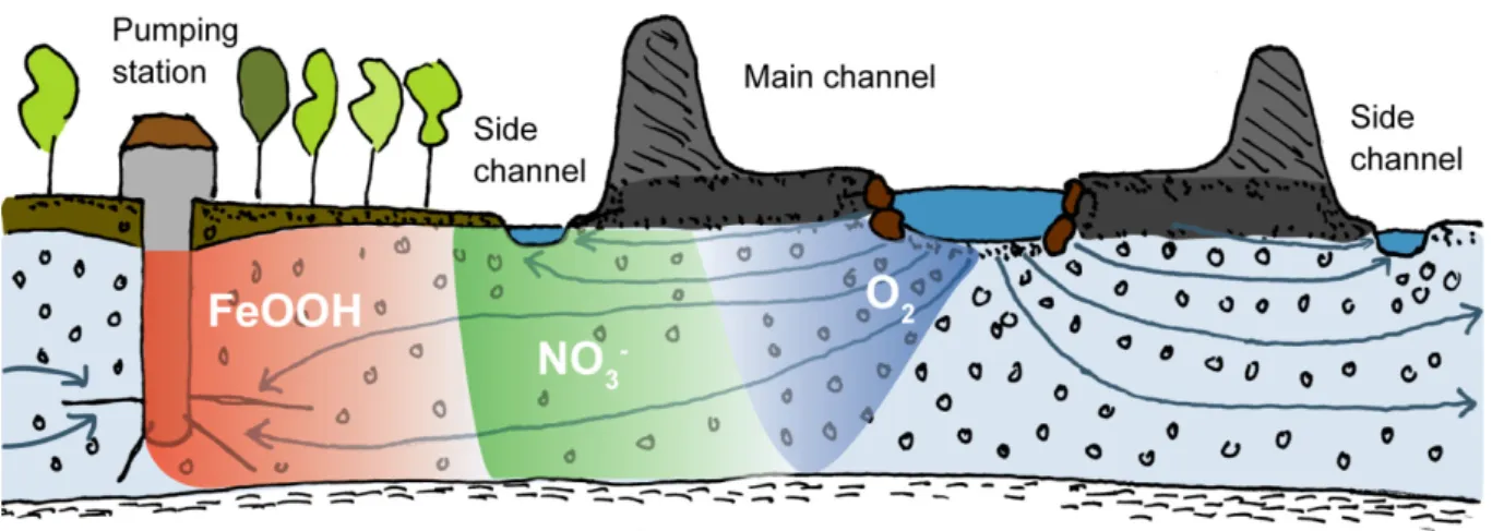
Low discharges are expected to increase groundwater residence times, as well as the loads of organic matter and nutrients in rivers due to less dilution of wastewater effluent (Sprenger et al., 2011). Combined with higher temperatures, summer heat waves tend to promote the development of anoxic conditions in the infiltration zone, as observed in summer 2003. An increased frequency and intensity of long-lasting heat waves is therefore likely to increase the risk for riverbank-filtration systems to become denitrifying or even Mn(IV)- or Fe(III)-reducing (Fig. 1.3) over periods of several months (Sprenger et al., 2011). Such long-lasting anoxic conditions would require complementary drinking water treatment technologies, the implementation of which is expensive and needs to be planned in advance to ensure the supply of high-quality drinking water. To assess the risk of arising anoxic conditions more accurately, it is crucial to understand the dynamics of NOM degradation during riverbank filtration and its dependence on the climate-related variables temperature and discharge. The quantification of these dependencies might allow for model-based estimates of oxygen concentrations in river-recharged groundwater, which would facilitate the anticipation of possible changes in redox conditions under various climatic and hydrologic conditions.
Fig. 1.3. Higher temperatures during future summer heat waves will enhance the microbial degradation of NOM, which might lead to a complete consumption of oxygen. In case of anoxic conditions, denitrification and eventually reductive dissolution of manganese and ferric oxyhydroxides can take place. The occurrence of nitrite and especially dissolved manganese and iron would require additional drinking water treatment steps. Furthermore, the re-oxidation of dissolved manganese and iron at the pumping well can lead to a clogging of the filter screen. Adapted from Schirmer (2013).
1.2 Objectives and structure of this thesis
The overall goal of this Ph.D. Thesis is to deepen the understanding of physical and biogeochemical processes affecting the quality of river-recharged groundwater, and to develop tools that may help to assess potential impacts of river restoration measures and climatic changes on the effectiveness of riverbank-filtration systems. This overall goal of the thesis was subdivided into four main objectives (i-iv), which will be addressed in Chapters 2-5, respectively. To achieve these objectives, an integrative approach was employed that combines field investigations, laboratory experiments, as well as groundwater flow and reactive transport modeling.
This thesis was written within the RIBACLIM project (RIverBAnk filtration under CLIMate change scenarios) in the framework of the National Research Program “Sustainable Water Management” (NRP61). Field investigations, method development and modeling work were performed at a partly restored field site in Niederneunforn (northeastern Switzerland) at the peri-alpine Thur River. Chapters 2-5 contain detailed descriptions of the field site.
Within the context of river restoration, the objectives of this Ph.D. Thesis were (i) to develop alternative methods to generate water level distributions of dynamic rivers for the application in groundwater models, and (ii) to assess the predictive capability of these methods with respect to the simulated groundwater residence time.
Chapter 2 presents two new alternative interpolation methods to estimate water level distributions of highly dynamic rivers in the context of modeling riverbank-filtration systems at scales in the order of kilometers. These methods were implemented at the Niederneunforn field site and water level time series at multiple locations within the river reach were generated. These water level predictions were compared with those of a third reference method, which is based on an existing hydraulic model, to test the accuracy of the alternative interpolation methods.
Chapter 3 investigates the impact of the method selection and the considered level of detail in the river water level distribution on the simulated groundwater residence time. Thereto, steady-state surface water level distributions were generated using both alternative methods, the reference method, as well as two simplified methods, and were assigned to a 3D groundwater flow and transport model of the field site. After calibration against groundwater heads, each of the models was used to predict the spatial groundwater residence time distribution within the modeling domain.
Within the context of climate change, the objectives of this Ph.D. Thesis were (iii) to investigate the dependence of NOM degradation during riverbank filtration on the climate-related variables temperature and discharge and (iv) to develop a model that simulates oxygen consumption during riverbank filtration as a function of river temperature and discharge. Chapter 4 elucidates the contribution of DOM consumption to the overall consumption of electron acceptors and its dependence on the climate-related variables temperature and discharge. Two detailed groundwater sampling campaigns were performed during typical summer and winter conditions to capture different temperature ranges. The results were compared to those of laboratory column experiments that were conducted at temperatures that span the range of the field conditions. Additionally, data of periodic field samplings that covered a wide range of temperature and discharge conditions over a period of five years were evaluated.
Chapter 5 presents a newly developed semi-analytical model that allows estimating oxygen concentrations in river-recharged groundwater under various climatic and hydrologic conditions. The model is based on the stochastic-convective reactive approach and incorporates a dependence of the oxygen consumption rate on river temperature and discharge. These dependencies were inferred from high-resolution oxygen time series measured in the Thur River and an adjacent observation well.
Chapter 2
New methods to estimate 2D water level distributions of
dynamic rivers
Published in Ground Water
Diem, S., Renard, P., Schirmer, M., 2012. New methods to estimate 2D water level distributions of dynamic rivers. Ground Water, doi: 10.1111/gwat.12005.
Abstract
River restoration measures are becoming increasingly popular and are leading to dynamic riverbed morphologies that in turn result in complex water level distributions in a river. Disconnected river branches, nonlinear longitudinal water level profiles and morphologically induced lateral water level gradients can evolve rapidly. The modeling of such river-groundwater systems is of high practical relevance in order to assess the impact of restoration measures on the exchange flux between a river and groundwater or on the residence times between a river and a pumping well. However, the model input includes a proper definition of the river boundary condition, which requires a detailed spatial and temporal river water level distribution. In this study, we present two new methods to estimate river water level distributions that are based directly on measured data. Comparing generated time series of water levels with those obtained by a hydraulic model as a reference, the new methods proved to offer an accurate and faster alternative with a simpler implementation.
2.1 Introduction
Over the past few decades there has been a shift in focus from river corridor channelization toward restoration. It has been recognized that rivers need more space for the purpose of flood protection (Woolsey et al., 2007). Furthermore, restoration measures such as widening of the riverbed, re-meandering stream reaches, and constructing gravel bars, should increase the exchange between rivers and groundwater, which is essential for the ecological health of a river (Brunke and Gonser, 1997). On the other hand, riverbed widening can decrease travel times between rivers and pumping wells, which may increase the risk of drinking water contamination by pollutants or bacteria (Hoehn and Scholtis, 2011).
Groundwater flow and transport modeling is a valuable tool to obtain a process-based understanding of (restored) surface water-groundwater systems. Compared to tools developed to work with artificial and natural tracers, a calibrated model provides quantitative conclusions on flow paths, mixing ratios and travel times (Wondzell et al., 2009). It is well known that riverbed morphology affects the river water level distribution, which in turn affects or drives the exchange with groundwater (Woessner, 2000; Cardenas et al., 2004; Cardenas, 2009). Therefore, one of the prerequisites for the setup of a groundwater flow model of a real river-groundwater system is an accurate description of the water level distribution in the river.
Restored river systems may have complex water level distributions that need to be characterized by their full spatial (i.e. two horizontal dimensions) and temporal extent (i.e. for any discharge condition). Past small-scale field and modeling studies (10 to 100 m) applied one or two sets of detailed water level measurements in one or two dimensions (Wroblicky et al., 1998; Storey et al., 2003; Lautz and Siegel, 2006; Wondzell et al., 2009). On the scale in the order of kilometers, which is more relevant for practical problems, this approach is not applicable. Instead, the extraction of river water level information from a hydraulic model might be a proper solution (Doppler et al., 2007; Derx et al., 2010; Engeler et al., 2011). However, the setup of a hydraulic model is time consuming and requires a large amount of data input, that is, the riverbed bathymetry and water level information for the calibration and validation process.
In this study, we present two alternative methods to estimate water level distributions of highly dynamic rivers in the context of modeling river-groundwater systems at scales in the order of kilometers. The two methods combine continuous and periodic water level measurements from different locations in order to account for the spatial and temporal
variability of the water level distribution. We predicted water levels at several locations at a restored reach of the peri-alpine Thur River and compared them with water level predictions of a reference method, which is based on an existing hydraulic model. Finally, we point out the advantages and disadvantages of the different methods and discuss the optimal use of each method when assigning the water level distribution of restored and dynamic river systems to groundwater flow and transport models.
2.2 Interpolation methods to estimate river water levels 2.2.1 Problem setup
Instrumentation of a 1 kmriver reach is typically comprised of two water level gauges, one upstream and one downstream of the field site. For groundwater flow modeling, river water levels need to be estimated at each river boundary node between the two gauging stations. The simplest method assumes a constant gradient (linear interpolation) in the longitudinal direction and a zero gradient in the lateral (transverse) direction. Although this might be adequate for a channelized system, for restored corridors the dynamic riverbed morphology might lead to a nonlinear longitudinal water level profile and to lateral water level gradients. Furthermore, the water level distribution might change as a function of the discharge.
The basic idea of the two new interpolation methods is to combine continuous water level records from water level gauges with water levels measured periodically under different discharge conditions. The latter are measured at “fixpoints”, which are distributed throughout the river reach to refine the water level distribution at locations where the installation of a water level gauge is technically difficult or simply too expensive. A fixpoint is defined as a reference point in the river, for example, a point on a construction rock or a steel rod, whose altitude is known. By establishing a mathematical relationship between the water level data at the gauging stations and the fixpoint, the water level at the fixpoint can be estimated for any measured water level at the gauging station.
We consider the river as a two-dimensional (2D) domain, which is discretized by multiple lines parallel to the main flow direction of the river and several sections of support points ( ) perpendicular to the flow direction (Fig. 2.1). The key task of the interpolation methods is to estimate a water level at each support point from any water level measured at the gauging station (i.e. for any discharge condition). Support points are placed at a location where a fixpoint ( ) or a gauging station ( ) exists. One fixpoint per section is enough unless lateral water level gradients are observed, in which case a fixpoint must be defined on both sides of
the river (Fig. 2.1). The periodic water level measurements at the fixpoints are denoted as , while the continuous water level measurements at the gauging station are denoted as . The estimation of consists of three steps:
1. Establish a mathematical relationship between the measurements and 2. Use to compute for any time step or time series:
3. Estimate the water levels or water level time series for the support points located on the same section as the fixpoint .
Different options for these steps have been considered for the two new methods, which are referred to as alternative methods. In order to compare these alternative methods with a reference, we developed a third method that is based on a hydraulic model and is referred to as the reference method. These three methods are described in the following sections. The explanation is descriptive in order to convey the main idea. A thorough mathematical development of the methods and their application to real data is presented in the Supporting information (Section 2.6).
Fig. 2.1. Schematic representation of a river system with multiple lines and sections of support points ( , black dots). Gauging stations ( ) and fixpoints ( ) are shown as black circles.
Once the set of lines and support points with water levels has been obtained using one of the three methods, the final interpolation of the water levels from the support points to the river boundary nodes of the numerical model has to be performed. This step is identical for all three methods and is accomplished by a one-dimensional linear interpolation along the lines, which implies that each of the lines is mapped by a curvilinear system of longitudinal coordinates to account for different curvatures of the lines. More precisely, each of the river boundary nodes of the groundwater model is projected perpendicularly onto the closest line and the water level is linearly interpolated between the upstream and downstream support point. Some simulation codes (e.g. FEFLOW) offer tools to accomplish this final interpolation step.
2.2.2 Method 1: Regression of measured data (RM)
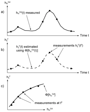
The first alternative method uses a polynomial regression technique to obtain the mathematical relationship . The method requires a continuous water level time series at one gauging station and periodic water level measurements at a fixpoint (Fig. 2.2). Each time a measurement is made at the fixpoint, the corresponding water level at the gauging station can be extracted from the continuous water level time series. A polynomial equation is then fitted to the data pairs, which constitutes the mathematical relationship . The polynomial order has to be chosen according to the range and the characteristics of the data. A guideline to defining the polynomial order is given in the Supporting information (Section 2.6). Applying to any water level time series measured at the gauging station produces predictions of corresponding water level time series at the fixpoint. If there are two fixpoints on the same section to capture lateral gradients, a separate polynomial equation is fitted to the corresponding data pairs. The gauging station is denoted as determining gauging station , as its water level uniquely defines the water level at the fixpoint.
Fig. 2.2. Illustration of the regression approach. (a) Continuous water level time series measured at the gauging station. (b) Periodic water level measurements at a fixpoint (black dots). For the same measurement times, water levels at the gauging station are extracted in (a). (c) is established between and by polynomial regression and is used to estimate the water level time series (dashed line) at the fixpoint in (b).
The estimation of the water level at the support points from the water level at the fixpoint is made in the simplest possible manner. If no lateral gradients exist, the water level of the fixpoint is assigned to all of the support points located on the same section. However, if a second fixpoint was installed on the same section to capture a lateral gradient, assigning the water levels to the support points should be based on field observations. For example, if a discrete step forms the lateral gradient, the water level at each support point can be determined from the most representative fixpoint. Otherwise, a linear interpolation between the two fixpoints might be an appropriate solution.
2.2.3 Method 2: Interpolation of measured data (IM)
The second alternative method uses an interpolation approach that requires two gauging stations. One of them has to be defined as determining gauging station . The fixpoints can be located between or outside of the two gauging stations.
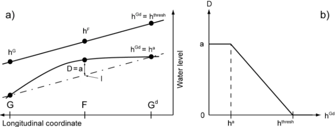
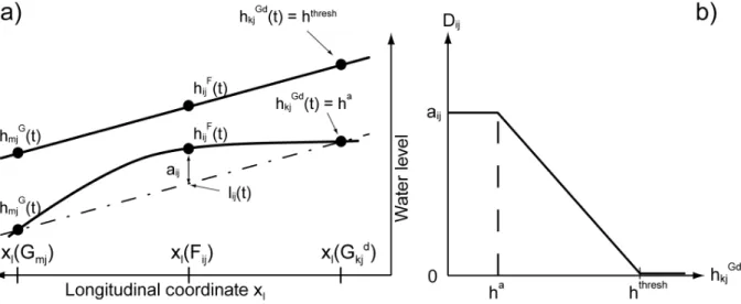
This IM method is based on a conceptual behavior model. According to the model, the riverbed morphology exerts a high influence on the river water level distribution under low-flow conditions, potentially leading to nonlinear longitudinal water level profiles or lateral water level gradients. As the water level rises, the influence of the riverbed morphology on the water level distribution decreases, and at some point lateral water level gradients disappear and a linear longitudinal water level profile is reached. In general, the IM method describes the water level at a fixpoint by an interpolation function ( ) that consists of a linear interpolation term between the water levels at the two gauging stations ( and ) and a deviation from the linear trend (Fig. 2.3). Following the conceptual behavior model, the deviation is at a maximum, , when water levels at the determining gauging station are smaller than . On the other hand, the deviation goes to zero for water levels higher than a threshold water level . Between and , the deviation is assumed to decrease linearly (Fig. 2.3). Similarly, we can describe the water level at a second fixpoint on the same section by the water level of the first fixpoint plus a lateral difference . Again, is at a maximum for low water levels and goes to zero above a threshold water level.
To estimate the parameters , and , the deviation from the linear trend has to be calculated for each measurement at a fixpoint and plotted against the corresponding water level at the determining gauging station. More details on how to estimate the parameters for the IM method are given in the Supporting information (Section 2.6). The estimation of the water level at the support points is identical to the procedure described in the previous section for the RM method.
Fig. 2.3. Illustration of the interpolation approach. (a) Two longitudinal water level profiles for the conditions and . (b) Deviation from the linear trend ( ) as a function of .
2.2.4 Method 3: Regression of hydraulic model data (RH)
To compare the two alternative methods with an independent reference, we developed a third method that is based on data from an existing hydraulic model of the main river channel in the section of interest. The hydraulic model output consists of 2D water level distributions, each corresponding to a specific discharge condition. Similar to the RM method, the RH method applies a polynomial regression technique to obtain the mathematical relationship . However, the relationships are based on water levels extracted from the hydraulic model output at each support point and at the location of the determining gauging station, and not on measured water levels.
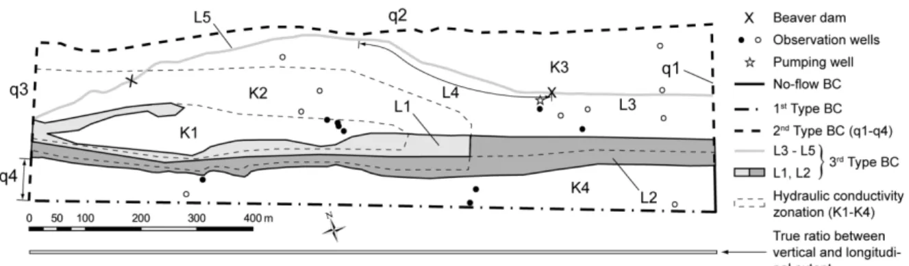
2.3 Application to the Niederneunforn field site 2.3.1 Field site
The peri-alpine Thur River drains a catchment area of 1730 km2 and originates in an alpine
region that reaches its highest point on Mount Säntis (2502 m above sea level, m asl). The Thur River is the largest river in Switzerland without a retention basin. This leads to a very dynamic discharge regime ranging from 3 to 1100 m3/s with an average of 47 m3/s. The field
site (Fig. 2.4) is located approximately 12 km upstream of the confluence with the Rhine River. In the western part of the field site, restoration measures were realized in 2002. Restoration measures were forbidden in the upstream section to protect the water quality at the nearby pumping station, where a pumping well supplies the community of Nieder- and Oberneunforn with drinking water. The field site was instrumented with more than 80 piezometers (2’’) during the interdisciplinary RECORD project (Restored corridor dynamics, http://www.cces.ethz.ch/projects/nature/Record; Schneider et al. (2011)). The aquifer has a
thickness of 5.3±1.2 m and its hydraulic conductivities were estimated to range from 4×10⁻³ to
4×10⁻² m/s (Diem et al., 2010; Doetsch et al., 2012). The silty sand of the alluvial fines on top of the aquifer has a much lower hydraulic conductivity and can be regarded as the semi-confining unit, with a thickness of 0.5-3 m.
The Thur River has a width of 50-100 m (Fig. 2.4). In the restored section a large gravel bar has evolved during the past few years. To the north, a disconnected branch of the river exists, which is only flooded at high river stages (>200 m3/s). The longitudinal river water level profile does not have a linear shape for low-flow conditions. In the upstream 400 m of the river the gradient is 0.5‰ and in the downstream 800 m it is 2‰. In the middle of the river reach, lateral water level gradients occur during low-flow conditions. These lateral surface water level differences exist due to the asymmetrical riverbed morphology and can reach up to 0.4 m. Two side channels (north and south) flow parallel to the river and have an average width of 4-8 m. Two beaver dams are located in the northern side channel. The upstream dam has a significant effect on water levels, creating differences of up to 0.5 m.
A 2D hydraulic model of the Thur River was developed by Pasquale et al. (2011) and forms the basis for the reference RH method (Section 2.2.4). Riverbed cross sections measured in September 2009 with an average spacing of 50 m were interpolated using the technique presented by Schäppi et al. (2010) to obtain the river bathymetry. The hydrodynamic simulations were performed using the 2D model BASEMENT, which applies the finite volume method to integrate the shallow water equations (Pasquale et al., 2011). The model deals with both sub- and supercritical flow regimes, thus providing a suitable tool to simulate 2D water level distributions of dynamic rivers. The modeling results comprise 19 steady-state simulations for flows ranging between 10 and 650 m3/s, and provide water level altitudes at each raster cell (2×2 m). The hydraulic model does not include the side channels and the disconnected branch and is considered to be valid until the major flood events of June 2010.
Fig. 2.4. Field site located in Niederneunforn at the Thur River with indicated lines, support points, fixpoints and gauging stations. Selected piezometers are shown as well. The white polygon shows the perimeter of method implementation.
2.3.2 Data collection and method implementation
We installed two water level gauges in the main channel of the river, as well as in both side channels, and one in the river branch (Fig. 2.4). Three of these water level gauges are maintained by the Agency for the Environment of the canton Thurgau. The sensors (DL/N 70, STS AG, Switzerland) have been continuously measuring pressure, temperature and electrical conductivity (EC) at 15-min intervals since April 2010 (error of single measurement: ±0.1% for pressure, ±0.25% for temperature and ±2% for EC, according to the manufacturer’s manual). We installed sensors of the same type in selected piezometers shown in Fig. 2.4. The raw data were processed in order to remove outliers, to subtract the barometric air pressure and to transform the pressure data to absolute water levels (m asl). To have more information on the water level distribution between the water level gauges, we installed several fixpoints along the river and the northern side channel. We chose the fixpoint positions according to the location of piezometer transects and visibly steep water level gradients (e.g. hydraulic jumps at beaver dams) or lateral gradients (central part of the river). We defined an indexing system that allows a distinct identification of each point. The first index refers to the section number and the second index to the line number. We leveled the absolute height of the fixpoints using a high-precision differential GPS (Leica GPS1200, Leica Geosystems AG, Switzerland) and a leveling device (Sprinter 100M, Leica Geosystems AG, Switzerland). We measured water levels at these fixpoints periodically between February and May 2011 covering a discharge range of 10 to 100 m3/s.
Based on the resulting data set, we implemented both alternative methods and the reference method, each of which covered the three steps described in Section 2.2.1. As the hydraulic model did not include the disconnected branch and the side channels, we coupled the RH method to the RM method. More details on the method implementation can be found in the Supporting information (Section 2.6).
2.3.3 Comparison of the interpolation methods
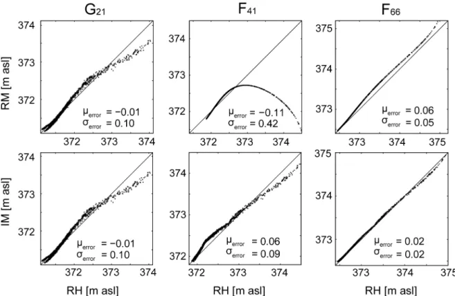
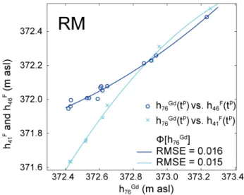
To evaluate the performance of the two alternative methods, we applied each of the interpolation methods (RM, IM, and RH) to generate water levels for a 1-month period (May 26, 2010 to June 30, 2010, vertical lines in Fig. 2.5) at each fixpoint and gauging station within the river domain. The upstream gauging station was used as the determining gauging station for each of the methods. We plotted the generated time series of water levels (30-min intervals) of the reference method (RH) against the time series of both alternative methods (RM and IM). Fig. 2.6 shows examples for one gauging station and two fixpoints. If
the generated water levels were the same for each time step, the dots of the scatter plots would be located on a line with a slope of one. Deviations from this line correspond to deviations of the RM/IM methods from the RH method and were quantified by a mean and a standard deviation (Fig. 2.6, Table 2.1).
Fig. 2.5. (a) Water level time series in the Thur River at fixpoint predicted with the RH method and measured groundwater heads in a nearby piezometer between May and October 2010. (b) Calculated water level difference between the river and groundwater. The vertical lines indicate the 1-month period used for creating the scatter plots of Fig. 2.6.
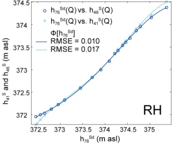
The scatter plots for the gauging station are identical for the RM and the IM method, which both used the gauging station data directly for this point. The water levels of the RH method however, were generated based on the hydraulic model. Therefore, these two plots actually compare the measured water level data with the water level predictions of the hydraulic model. The match was good for lower water levels but deviations of up to 0.5 m occurred for the peak flows during flood events. As only a small portion of the data was subject to such large errors, the mean error of water level prediction with the RH method was small (1 cm). The uncertainty of the water level prediction is reflected in the standard deviation of 10 cm (Table 2.1).
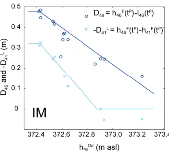
The scatter plots of the fixpoint revealed a difference in the behavior of the two alternative methods. The water level predictions for the study period (Fig. 2.5) exceeded the range of water levels measured at (371.6-372.5 m asl). Depending on the polynomial fit, the RM method is likely to fail for predictions outside of the measured range, as there are no data points constraining the polynomial equation. In our case, the parabola that was fitted to the data at the fixpoint was obviously too narrow in order to reliably predict water levels beyond the measured range. Correspondingly, the deviations with respect to the RH method
showed a mean error of -11 cm and a standard deviation of 42 cm. The IM method performed better for the peak flow water levels. As the water level predictions at a fixpoint are always bounded by two measured water levels at the upstream and downstream gauge, the stability beyond the measured range was better for the IM method. For the fixpoint , both the RM and the IM method performed well despite the systematic positive offset for the RM method at high water levels. This offset might be attributed to the problem described above for the fixpoint .
Most of the mean errors and their standard deviations for the fixpoints within the river domain varied between 1 and 10 cm (Table 2.1). We considered this level of error to be acceptable as the reference RH method itself had an accuracy of ±10 cm at . As was the determining gauging station for all fixpoints in the river, predictions were identical for all methods, explaining the values of zero in Table 2.1. The high standard deviations for the fixpoints and for the RM method can be blamed on the failure of the regression approach beyond the measured data.
Fig. 2.6. Scatter plots for one gauging station ( ) and two fixpoints ( , ) within the river domain. The time series of water levels generated by the reference method RH are plotted against the time series of water levels generated by the RM (top three figures) and the IM method (bottom three figures). Mean (µerror) and standard deviations (σerror) of the
The alternative methods – especially the IM method – tend to show higher deviations (>10 cm) from the RH method at the fixpoints on sections 1 to 4, which are located in the restored part of the river. We found evidence that the major flood event on June 17 through 24, 2010 (Fig. 2.5) led to a change in the riverbed morphology in the restored river section and to a corresponding change in the relationship between the water levels at the determining gauging station and at the fixpoints. First, the scatter plot for the gauging station (Fig. 2.6) reveals two distinct regimes at the lower end of the water level spectrum for the 1-month period that covers the major flood event. Second, after the flood event there is a clear and permanent decrease (~10 cm) in the difference between the water levels at predicted with the RH method, and groundwater heads measured at a nearby piezometer (Fig. 2.5). The drop in the water level difference could be due to a change in the riverbed morphology after the flood, resulting in an underprediction of water levels by the RH method, which assumed a constant morphology. Because the data for the RM and the IM method were collected after this morphologically active flood event, they might have captured the higher water levels and accordingly led to an overestimation of water levels compared to the RH method. Therefore, the differences in predicted water levels among the different methods were presumably not only caused by structural artifacts, but also by real differences due to morphology changes in the river.
Table 2.1. Mean (µerror) and standard deviations (σerror) of the residuals [m] between the time
series of water levels generated by both alternative methods and the reference method at the gauging stations and fixpoints within the river domain.
RM F18 G21 F36 F31 F46 F41 F51 F66 G76 µerror 0.07 -0.01 0.05 0.06 -0.08 -0.11 -0.01 0.06 0.00 σerror 0.12 0.10 0.04 0.04 0.42 0.42 0.07 0.05 0.00 IM F18 G21 F36 F31 F46 F41 F51 F66 G76 µerror 0.11 -0.01 0.16 0.17 0.12 0.06 -0.04 0.02 0.00 σerror 0.16 0.10 0.09 0.08 0.08 0.09 0.04 0.02 0.00 2.4 Discussion
A hydraulic model has the advantage of being physically based, which allows a wide range of discharge conditions to be simulated. This makes water level predictions by the RH approach very robust. However, setting up a hydraulic model is time consuming, and needs both a large data set and to be thoroughly calibrated. At our field site, the hydraulic model was not able to include the water levels of the disconnected river branch, because during low-flow conditions this branch is fed by groundwater. Furthermore, the hydraulic model did not cover the side
channels. The RH method had to be coupled to the RM method in order to include the full surface water level distribution required for the assignment of boundary conditions in a groundwater model.
Compared to the RH method, both alternative methods presented in this chapter (RM and IM) provide a more efficient way of predicting water level distributions in a hydraulically and morphologically varying environment. First, the accuracy of the water level predictions with the alternative methods was in the same range as the accuracy of the reference RH method itself. Second, the alternative methods require minimal data and computational effort, making them simpler and faster to implement than the hydraulic model.
In comparison to the IM method, the RM method benefits from the regression approach, which is fast and straightforward in its implementation and its application. However, the RM method does not provide reliable water level predictions when they exceed the range of water levels measured at the fixpoints. This in turn is the strength of the IM method, whose water level predictions are always bounded by water levels measured at two gauging stations. Furthermore, the IM method is based on a conceptual behavior model that is physically consistent. Even though the IM method is empirical and more complex in its implementation, the measured data at most of the fixpoints supported the method’s underlying assumptions.
2.5 Conclusions
Several field and modeling studies have shown that the water level distribution in rivers exerts an important influence on the exchange between rivers and groundwater. In this study, we presented two new methods to define spatial and temporal river water level distributions for the purpose of modeling surface water-groundwater systems. The basic idea is to record water levels continuously at water level gauges and measure water levels periodically under different discharge conditions at fixpoints to refine the water level distribution at locations where it is technically difficult or too expensive to install a gauging station. The RM method applies a polynomial regression approach for the prediction of water levels at fixpoints as a function of the corresponding water levels at the determining gauging station, while the IM method uses an interpolation approach between two gauging stations. To compare these alternative methods to a reference method, we developed a third method, which is based on water level data from a 2D hydraulic model and also applies a regression approach (RH). The hydraulic model has the clear advantage of being physically based and covering a wide range of discharge. On the other hand, the alternative methods are simpler and faster in their implementation, while still being able to account for typical hydromorphological features of
dynamic (restored or natural) river sections (e.g. nonlinear longitudinal water level distributions, lateral water level gradients, disconnected river branches and hydraulic jumps). We compared water level time series generated by both alternative methods with those generated by the reference method at all of the fixpoints located in the 1.2 km long river reach of our field site. For most cases, the accuracy of the water level predictions of the alternative methods was comparable to the accuracy of the reference method itself. In addition, we found evidence that the riverbed, and hence the water level distribution for a given discharge condition, changed between the implementation of the reference and the alternative methods. This change in riverbed morphology might have contributed to some of the larger deviations among water level predictions.
The results of this study allow us to recommend both alternative methods for the river water level assignment in future modeling studies of river-groundwater systems at scales in the order of kilometers. The RM method is straightforward in its implementation, but is limited to water level predictions within the range of measurements made at the fixpoints. If discharge conditions beyond the measured range have to be simulated, we recommend the use of the IM method instead.
Each of the presented methods has limitations in terms of accuracy in water level predictions. Even though we consider each of the methods to be accurate, water level predictions will differ for a specific discharge condition. The impact of the river water level uncertainty on key predictions of groundwater models as exchange flux or groundwater residence time, both in steady state and transient conditions, could be the basis for future research.
Acknowledgments
This study was accomplished within the National Research Program “Sustainable Water Management” (NRP61) and funded by the Swiss National Science Foundation (SNF, Project No. 406140-125856). Many thanks to Matthias Rudolf von Rohr, Lena Froyland, and Urs von Gunten for their support. We would like to thank Nicola Pasquale (IfU, ETH Zurich) for having provided the results of the hydraulic model. We thank John Molson and Ryan North for many helpful discussions. The Agency for the Environment of the canton Thurgau provided data, logistics and financial support. Additional support was provided by the Competence Center Environment and Sustainability (CCES) of the ETH domain in the framework of the RECORD project (Assessment and Modeling of Coupled Ecological and Hydrological Dynamics in the Restored Corridor of a River (Restored Corridor Dynamics)). We thank the three anonymous reviewers for their constructive comments.
2.6 Supporting information
This section contains a detailed description of the interpolation methods and their implementation at the Niederneunforn field site.
2.6.1 Problem setup
At our field site, we considered the river as a two-dimensional domain and the two side channels as a one-dimensional domain, based on their different widths. The river geometry was represented by a set of six lines for the main channel plus one line for the disconnected branch. Both side channels were represented by one line (Fig. 2.7). A more general and schematic river system is illustrated in Fig. 2.8. We consider now that each of the lines is mapped by a curvilinear system of longitudinal coordinates . The lines were numbered with an index for the main river channel in our example. Similarly, sections perpendicular to the main course of the river were considered and numbered with another index . The same numbering system was used for the river branch and the side channels with the line indices .
Fig. 2.7. Field site located in Niederneunforn at the Thur River with indicated lines, support points, fixpoints and gauging stations. The colors of the support points indicate the line/fixpoint, from which the water level was transferred. The general flow direction in the river and the side channels is from right to left.
The intersections between the lines and the sections (Fig. 2.8) define the locations of support points where water levels will be estimated using the interpolation methods described below. Support points are identified in this coordinate system with a letter and two indices, . The first index always refers to the section number and the second index always refers to the line number.
Fig. 2.8. Schematic representation of a curvilinear coordinate system with the lines and the sections . The dots at intersections between the lines and the sections represent support points and the circles represent gauging stations or fixpoints
.
represents a gauging station located on section and line where water levels are measured continuously. represents a fixpoint on section and line with periodic manual measurements. Their curvilinear coordinates are denoted and , respectively. The measured water levels are denoted as for those continuously recorded at , and
for those recorded periodically at fixed times at . The longitudinal position of the sections perpendicular to the main river axis are chosen such that each section contains at least one fixpoint or gauging station.
The aim of the interpolation methods is to estimate the water levels at any support point , where only limited or no water level data is available, by combining the measured water levels at a gauging station with those at a fixpoint . The indices and have the same meaning as but refer to a different location within the coordinate system. The estimation of is comprised of three steps.
1. Establish a mathematical relationship , such that . 2. Use to compute for any time step : .
3. Estimate the water levels for the support points located on section and lines and , based on .
Different options for these steps have been considered for the two new methods, which are both based on measured data at gauging stations and fixpoints and are referred to as alternative methods. In order to compare these alternative methods with a reference, we developed a third method, which is based on a hydraulic model and is referred to as reference method. These three methods are described in the following sections. All three methods have been implemented in a MATLAB program. The final interpolation of the water levels from