Estimation in Surveys Using Conditional Inclusion Probabilities: Simple Random Sampling

Key words: Simple random sampling; Conditional estimation; Weighted observation.

1 Introduction

In survey sampling theory, conditional inference has been discussed especially in the context of post-stratification. Holt & Smith (1979) advocate in this case that "inferences should be made on the achieved sample configuration of the sample post-stratum frequencies". They argue for conditional inference after selecting the sample and point out that the post-stratified estimator "offers protection against extreme sample configurations". Other authors have considered how to obtain estimators which have small or no conditional bias. The idea of suppressing the conditional bias has been applied to the ratio estimator by Robinson (1987) who computes the conditional bias of the ratio estimator un der assumptions of normality and then corrects it by using an estimator of the conditional bias. The computation and estimation of the conditional bias is presented as an estimation principle by Rao (1985) who applies a conditional bias adjustment to the mean estimator, the ratio estimator in simple random sampling and stratified sampling design and for domain estimation. More recently Rao (1994) has given a general set-up for estimation using auxiliary information and compares the calibration methods to the conditional approach. The aim of this paper is to propose a general estimator based on conditional inclusion probabilities that allows us to construct directly an estimator with a small conditional bias with respect to a statistic. lt is also shown that many classical estimators used in survey sampling can be derived from this general estimator.

Before defining this general estimator, we give an example to show that the basic idea of conditional estimation is very intuitive. Suppose that a sample of size n

=

200 is drawn by means of simple random sampling in a population of size N

=

2000 composed of N1

=

1000 males and N2

=

1000

Estimation in Surveys Using Conditional

Inclusion Probabilities: Simple Random

Sampling

Yves Tillé

CR ST - SAI, École ationale de la Statistique et de ['Analyse de l'Information, rue Blaise Pascal, Campus de Ker Lann, 35170 Bruz, France. e-mail: [email protected]

Summary

In survey sampling, auxiliary information on the population is often available. The aim of this paper is to develop a method which allows one to take into account such auxiliary information at the estimation stage by means of conditional bias adjustment. The basic idea is to attempt to construct a conditionally unbiased estimator. Four estimators that have a small conditional bias with respect to a statistic are proposed. lt is shown that many of the estimators used in the literature in the case of simple random sampling can be obtained by using this estimation principle. The problem of simple random sampling with replacement, poststratification, and adjustment of a 2 x 2 dimensional

contingency table to marginal totals are discussed in the conditional framework. Finally it is shown that the regression estimator can be viewed as an approximation of an application of the conditional principle.

females. The aim is to estimate the average height

z

in the population. Denote by

z

I and z2 respectively the male and female average heights and suppose that the sample obtained is composed of n 1

=

90 males of average height i1

=

172 and n2

=

110 females of average height i2

=

164. Two estimators can be used to estimate the average height.

or � n1 x ZI

+

n2 x z2 172 x 90

+

164 x 110 6 ,ZA

=

n

=

200

=

1 7 .6, � NI X

I1

+

N2 X 12 172 X 1000

+

164 X 1000 Zn =

=

=

168.

N

2000 (1)

(2)

Estimator

in

looks more appropriate than

i

A because it includes a correction with respect to the real

ratio males/females. Estimator

i

A is the usual sample mean which is unconditionally unbiased for

i

A

,

but which is biased conditional on the number of males and females in the sample. Estimator

in

is well-known to survey statisticians and is called the poststratified estimator, is unconditionally unbiased for

z

and has a very slight conditional bias. We show below that the poststratified estimator can be obtained from the sample mean by a conditional bias adjustment. The aim of the paper is to formalise this idea and to show that, in survey sampling, many classical estimators can be viewed also as applications of a similar conditional bias adjustment.

The opportunity to apply a conditional bias adjustment ensues practically from the existence of auxiliary information that allows us to estimate a conditional expectation with respect to a statistic. We shall refer to this statistic as an auxiliary statistic and denote it by TJ. The objective is to decrease the variance of an estimator in the following way. Let ê be an unbiased estimator of a parameter e. If B ( ê

1

7J)

=

E ( ê

1

7J) - e, the condition al bias of ê given 7/ is known, it is possible to construct the adjusted estimator ê*

=

ê - B(ê

I

TJ). We gel

Since

we obtain

Var(ê*)

=

Var(ê)

+

Var {B(ê

I

7/)}- 2Cov

{ê,

B(ê

1

7/)}. Cov(ê, B(ê

I

7/))

= .

EE { (ê - e)(E(ê

1

7/) - e)

1

7/}

Var {E(ê

I

7/)},

Var(ê*)

=

Var(ê) - Var {E(ê

I

7/)}. _'(3)

The variance of the adjusted estimator ê* will thus be no greater than that of the original estimator ê. The problem of this approach is that the conditional bias must in general be estimated, and that the benefits gained in attempting to decrease the conditional bias could be thwarted by the instability of the conditional bias estimator used.

This approach can be applied to the estimator

i

A defined in ( 1 ). If the statistic used to compute

the conditional bias is 7/

=

(n1, n2), and if it is supposed that the probability of obtaining an empty poststratum is negligible, we obtain

and thus

� 1

which can be estimated by

�r?

1

1 � � 1 � �

B lZA ni, n2)

= -

_n (niz1

+

n2z2} - - (Nizi _N

+

N2z2). Finally we obtain the adjusted estimator

ZA

-

Ê(zAln1, n2}

=

ZB·

Estimator ZB is thus obtained from ZA by suppressing the conditional bias.

The approach proposed in this paper is a formalization of an approach that appears in numerous publications about survey sampling. The construction of a conditionally unbiased estimator is treated as a technique to develop a more precise estimator. The original feature of this paper is that, instead of obtaining ê* from ê by a conditional bias adjustment, we propose to construct conditionally un­ biased estimators directly using conditional inclusion probabilities. The existence of a conditionally unbiased estimator with respect to a statistic is discussed in Section 2. Four conditionally unbiased estimators are proposed. These estimators generalise the poststratified estimators and can be used to build a method of adjustment of a 2 x 2 table to known marginal totals (Section 3). Next it is shown that the regression estimator is an approximation of one of these estimators (Section 4). Finally the issues of conditional bias adjustment is discussed in Section 5.

2 Conditionally Unbiased Estimators

2. I Existence of a Conditionally Unbiased Estimator

Suppose that a random sample S is drawn without replacement from a finite population U {l, ... , k, ... , N} following a sampling design p(.). The probability of selecting the sample s is Pr(S

=

s)

=

p(s) for ail non-empty s C U. The indicator variables h take the value 1 if unit k is in the sample and O if not, for ail k E U. The probability that unit k is selected is JCk

=

E(h)

and is called the first-order inclusion probability. The probability of selecting both units k and l is Jeu

=

_{E(hle.) and is called the second-order inclusion probability. Consider Yk and Xk, respectively} the value of the variable of interest y and the value of the auxiliary variable x on the kth unit. The values Xk are assumed known for ail k E U.

is

The Horvitz-Thompson estimator ( 1952) of the mean

- 1 Y = N LY_kEU k (4) " 1 '"' Yk

Y

1r

= -

_N L.., -. kES 1Ck

Let 7J

=

TJ(Xk, k E S) be a statistic. Since the population is finite, the statistic 7/ takes a finite number of possible values denoted {7/1, ••• , TJ;, ... , T/1 }. The objective is to estimate ji with a conditional bias as small as possible with respect to TJ. Define the first-order conditional inclusion probabilities to be 7rkJ,,

=

E(h I TJ) for ail k E U and the conditional joint inclusion probabilities to be

7rkfl�

=

E(hlr

1

7/) for ail k E U, l E U, k # l.

An estimator constructed with conditional inclusion probabilities will be called a conditionally weighted (CW) estimator. First, we introduce the simple CW (SCW) estimator given by

(5) The conditional inclusion probabilities are assumed to be calculable for any possible value of TJ. The

statistic 7/ is called the auxiliary statistic. The conditional bias of the SCW-estimator is given by : B(.Y1 11

1

7/)

=

E(y,.,

1

7/) - Y

=

_!_

L

E ( Ykh 17/) - y N kEU 1l'kl11 1l"tJ,,>0 1

= --

_N LYkl[rrk111

=

0), kEU

where /[.] is the indicator fonction given by

/[rrkl11 = 0) = { _{0 ifrrkl., > O.} 1 ifrrkl.,

=

0

(6)

Remember that a well-known result of sampling theory is that a necessary condition for the existence of an unbiased estimator of y is that 1Z'k > 0, for ail k E U. This result can be transposed

conditionally to 7/ and gives that a necessary condition for the existence of a conditionally unbiased estimator of y is that rrkl'I > 0, for ail k E U, and for ail possible values of 7].

Note that in the general case, (see Example 2) the conditional inclusion probabilities can take the value O even if the unconditional inclusion probabilities are strictly positive and thus an ex­ actly conditionally unbiased estimator generally does not exist. A weaker definition of conditional unbiasedness will also be considered.

DEFINITION 1: An estimator of y denoted

y

is said to be virtually conditionally unbiased (VCU)

with respect to a statistic 7J if

B(y

1

7/)

=

L YkŒk(TJ)l (1Tkl11

=

0),

kEU

for all _{(y1 ... Yk ... YN)} E RN, where the coefficients ak(TJ) can depend on TJ.

When an estimator is VCU, this does not necessarily imply that the conditional bias is near zero but that the conditional bias only depends on the units having null conditional inclusion probabilities. Expression (6) directly shows that the SCW-estimator is VCU.

EXAMPLE 1: If a simple random sample is drawn without replacement from a population of size N with random size ns where ns > 0, then if 7J

=

ns, we obtain rrkl'I

=

E(hlns)

=

ns/ N, k E U.

Since ns/ N > 0, k E U, an exactly conditionally unbiased estimator with respect to ns always

exists.

EXAMPLE 2: If a simple random sample of size n

=

2 is drawn without replacement from a population U

= {

_{1, 2, 3, 4, 5} of size N}

=

5 and if the statistic used is

7/

=

k1 + k2

where k1 and k2 are the index numbers of the two units drawn in the sample, the possible values for the conditional inclusion probabilities are given in Table 1.

Table 1

Conditional inclusion probabilities: Example 2

values of 71'kl� 1/i Pr(TJ

=

11;) k=I 2 3 4 5 3 1/10 1 0 0 0 4 1/10 0 0 0 5 1/5 1/2 1/2 1/2 1/2 0 6 1/5 1/2 1/2 0 1/2 1/2 7 1/5 0 1/2 1/2 1/2 1/2 8 1/10 0 0 0 9 1/10 0 0 0

So, if TJ takes the value 5, either the sample { 1, 4} or {2, 3} was selected, thus E[Js l TJ

=

5]

=

0, and E[h I TJ

=

5]

=

1 /2, k -=1-5. In this case, many conditional inclusion probabilities equal zero and thus an exactly conditionally unbiased estimator does not exist in the class of linear estimators. 2.2 Other Conditionally Weighted Estimators

It is possible to derive other CW-estimators. First, it is always possible to construct an uncondi­ tionally unbiased estimator given by

where

hk = EI[rrklry > 0] = Pr (rrklry > 0).

Estimator (7) will be called the corrected CW (CCW) estimator. lts conditional bias is � _{_!__ � Yk ( J[rrklry > 0] -}

1) .

B(Yc1,,l11)

=

_{N � h}

kEU k

The CCW-estimator is not VCU but it is unconditionally unbiased. Indeed, by (8), we get B(Yclry)

=

EB(Yclry

I

TJ)

=

O.

(7)

(8)

Both SCW and CCW-estimators can be criticised because they are not invariant by translation, i.e. these estimators do not increase by a value C when all the units Yk are increased by a value C. Indeed, for the SCW-estimator, we obtain

1 � Yk

+

C " C � l "

N �-- = Y_c1

ry+ N �--=1-Yclry+C.

kES 1l'k_{lry kES} 1l'k_lry

To solve this problem, two 'ratio' versions of Yiry and Yclry can be constructed.

1. the SCW-ratio

2. the CCW-ratio

( )-1

" � 1 � Yk

Y,1ry= _{�- �-,}

kES 1l'k_{lry kES} 1l'k_lry

( )-1

" � 1 � Yk

Ycrlry = �-- �--.

kES hk1l'k_{lry kES hk}1l'k_lry

(9)

They are invariant by translation. This property is appreciated by practitioners who consider it is more important to have an estimator where all the sums of percentages equal one hundred than a conditionally unbiased one. An approximation of their bias and conditional bias can be found by means of the linearization technique used for the research of a bias in the classical ratio estimator (see for instance Cochran, 1977, p. 161).

Among the four CW-estimators, which one should be chosen? Since a conditionally unbiased estimator rarely exists, it will usually be necessary to allow for a slight conditional bias. lt is also interesting to note that it is always possible to correct the CW-estimator in order that it be uncondi­ tionally unbiased. Nevertheless, this correction enlarges the conditional bias and thus increases the MSE. For this reason, we prefer to use the estimator (5) and (9). We advocate the use of SCW-ratio when the sum of the inverses of the inclusion probabilities is not equal to N.

2.3 Conditional Inclusion Probabilities

To construct the CW-estimators, the conditional inclusion probabilities must be evaluated. Using Bayes's theorem, we obtain

E(h

I

T/

=

r,;)

=

Pr(k ES

I

T/

=

r,;) Pr(r,

=

T/i

I

k E S)

=

7rk , z

=

1, ... , /.

Pr(r,

=

T/i)

To compute the conditional inclusion probability, the probability distribution of T/ unconditionally and conditionally on the presence of each unit in the sample must be known. In the perspective of conditionally weighted estimation, the auxiliary information required is the knowledge of the probability distribution of the auxiliary statistic T/. The probability distribution of T/ can theoretically be derived from the sampling design. Indeed,

and Pr(r,

=

r,;)

=

L

p(s) si�=�; Pr(r,

=

T/i I\ k E S) _{1 �} Pr(r,

=

T/i I k E S)

=

= - �

p(s). 1fk _{1fk si�=�;} s=>k

In practice, it is far from self-evident exactly how the conditional inclusion probabilities are to be computed. We shall see that, in some cases, conditional inclusion probabilities can be calculated exactly; in other cases, approximations must be used.

3 Applications to Simple Random Sampling 3.1 Sampling with Replacement

One of the simplest applications of CW-estimators occurs in simple random sampling with re­ placement. Consider the following classical problem: m units are drawn with replacement with equal probabilities from a population of size N. The resulting sample is composed of the ns distinct units. 1t is known (see Basu, 1958, Raj & Khamis, 1958, Pathak, 1961, Konijn, 1973, chap. IV, and Rao 1985) that

and ( (N - l)m) E(ns)

=

N l - _Nm (N - 1r (N - 2r (N - 1)2m Var(ns)

=

Nm-1

+

(N - 1) Nm-1 N2m-2 . (11) (12) Suppose now that ns is used as the auxiliary statistic. Since, conditionally on ns, the design is with equal probabilities and without replacement, we get 7rklns

=

E(h

I

ns)

=

ns/N for all k E U. The unconditional inclusion probabilities are E(1rk1ns>

=

N-1 E(ns)

=

(1- N-m(N - Ir). Moreover Pr(rrklns > 0)

=

1 and thus the four CW-estimators are all equal to the simple sample mean

_Y

₁

_�

=

.Ys

=

n

s

1

LkES Yk while the Horvitz-Thompson estimator is given by

- _ ___!!_!_- - N l-

'°'

� _{{ (} (N-l)m

)}-1

Yrr - E(ns) Ys - Nm _�

fu

Yk·

Note that .Ys is unbiased conditionally on ns while Yrr is not. Moreover, .Ys is invariant by translation while

y

rr is not.

Konijn (1973, Chap IV), proved that the variance of the CW-estimator is given by

where

V [-] E a.Y ( -ns cr.Y L.j=I J 2 N ₎ 2 '\'N-1 ·m-1 ar Ys = -_{ns N - l} = -_{m Nm-1} 2 l" -2 ay

=

N L..., (Yk - y) kEU

The variance of the Horvitz-Thompson estimator is given by Var[yrr] Var --ys [ _E(ns) ns _ ]

=

EV ar [ ___!!_!_.Ys I ns] _E(ns)

+

Var E [___!!_!__.Ys! ns]_E(ns)

a; ( N E[ni] ) ji2

= -- ---

+--Var[ns]

N - 1 E[ns] E[nsF E[nsF

(13)

(14) where ns is defined as in (11). Examining (13) and (14), we see that the CW-estimator has a smaller variance if and only if

_2 a; { E[ns ]2

( [ 1 '] 1 ) 1}

y>--·- NE----+

N - 1 Var[ns] ns E[ns] ·

This application is interesting. lt shows that, even in case all the conditionaJ inclusion probabilities are larger than zero, the CW-estimator has not necessarily a smaller variance than the Horvitz­ Thompson estimator. lndeed, for this example, the Horvitz-Thompson estimator has a smaller variance if the population mean is close to zero. This simple result shows that it is impossible to determine the best estimation procedure without taking into account the relation between the auxiliary statistic and the interest variable.

This result cou Id appear to be in contradiction to expression (3) that shows that if the conditional bias is corrected, the variance of the estimator will be smaller. Nevertheless, as we write in Section l, the benefit gained in attempting to decrease the conditional bias could be thwarted by the instability of the conditional bias estimator used. For this reason, the CW-estimators are not better than the Horvitz-Thompson estimator for ail possible values of ji.

3.2 Poststratification

Suppose that a simple random sample of size n is drawn without replacement from a population of size N. The population is assumed to be divided into H poststrata Uh, h

=

1, ... , H, of sizes

Nh, h = 1, ... , H. We denote nh, h = 1, ... , H, the sample poststratum sizes. Since the sampling

design is simple without replacement, rrk

=

n / N for all k E U. Suppose now that 7/

=

(n1 ... nh ... nH ). Note that

(N)-I

H (Nh₎

Pr(nh=rh,h=l, ... ,H)= _n

n

,

h=I rh

where rh = 0, ... , Nh, I:f=l rh = n, and, if k E Ua,

Pr(nh = rh, h = 1, ... , H I k ES)

=

(N -1)-

1(Na

-1)

Il

(Nh)·

n - 1 ra - 1 _{h=I r}h h#a

lt follows that 7rkl� =na/Na and

(N - Na)lnl

Pr(rrkl� > 0) = 1 - Pr[na = 0] = 1 - _Nin]

where Nlnl

=

N(N - 1) ... (N - n

+

1). The four CW-estimators become

1. from (5), the SCW-estimator

2. from (7), the CCW-estimator

"- 1 H NhyhNln]

Yci�

=

_N

L

_{Nin]_ (N _ N )ln]'} 3. from (9), the SCW-ratio

4. from (10), the CCW-ratio

h=I h

nh>O

where Yh denotes the simple sample mean within the hth poststratum.

(15)

(16)

(17)

(18)

by Holt & Smith (1979). Doss, Hartley & Somayajulu (1979) discuss estimator (16) which is exactly unconditionally unbiased but not VCU. In the same paper, these authors discuss CCW-ratio (18). An interesting discussion of these estimators is given by Rao (1985). In practice, we advocate the use of SCW-ratio because it is invariant by translation and, if nh > 0, h

=

1, . . . , H, it is calibrated on the Nh i.e. if the SCW-ratio is used to estimate Nh, one gets exactly Nh.

3.3 2 x 2 Contingency Tables

A classical application of the use of auxiliary information occurs in modifying cell estimates in a contingency table with the aid of known marginal counts. The application of CW-estimator to this case is rather complex. For this reason, we only consider a 2 x 2 contingency table. Suppose that the population is divided into four subpopulations Uh_q, h

=

1, 2, q

=

1, 2, of size Nh_q, h

=

1, 2, q

=

1, 2. We also denote Nh.

=

Nh1

+

Nh2, h

=

1, 2, and N._q

=

N_1q

+

N2_q, q

=

1, 2. In the population, only the marginal totals of the table are assumed to be known.

Suppose that a sample of size n is drawn with a simple random sampling design without replace­ ment and that the number of units selected in each subpopulation is denoted nh_q, h = 1, 2, q = 1, 2, with nh. � nh1

+

nh2, h

=

1, 2, and n._q

=

n_1q

+

n2_q, q

=

1, 2. The Horvitz-Thompson estimator of N11 is N11,r

=

Nn11/n. However, the objective is to construct an estimator of N11 that takes into account the auxiliary information given by the marginal totals of the population.

Generally this problem is viewed as a calibration problem. The sample contingency table is adjusted to the marginal totals of the population table. (See, e.g., Stephan, 1942, Frielander, 1961, Ireland & Kullback, 1968, Fienberg, 1970, Thionet, 1959 and 1976, Froment & Lenclud, 1976, Durieux & Payen, 1976). The estimator obtained by applying such an adjustment is usually called a raking ratio estimator.

The interest fonction Nu is a total as in (4) and can thus be estimated by a SCW-estimator. The following result gives a VCU-estimator of N11 with respect to the auxiliary statistic (n1., n.1) by using a SCW-estimator.

RESULT 1: The SCW-estimator of N11 with respect to T/

=

(n1., n.1) is given by

(19) where

1/l(N11, z)

Nf�l(N1. _ Nu)lni.-zl(N.i _ Nu)ln.1-zl(N _ N.i _ N1.

+

Nu)ln-n1.-n.1+z]

=

_z!(n 1. - z)!(n., - z)!(n - n1. - n.1

+

z)! (20) b-

=

max(O, n1.

+

n.1 - n, N11 - N1.

+

n.1, N11 - N.1

+

ni) (21) and b+

=

_{min(n1., n.1, N11, N - N1. - N.1}

+

_N11

+

_n1.

+

_{n.1 - n). (22)}

The proof is given in Appendix 1.

Note that this estimator (19) depends on Nu, which we want to estimate. It is thus impossible to construct a CW-estimator without knowing Nu. As the problem cannot be solved when only the marginal totals are known, we must use an aprroximation. The estimator that best respects the idea of suppression of conditional bias is denoted

N

u1., and satisfies the relation

Knowing that

N u1., E [max(nu, N1.

+

N.1 - N

+

n - n1. - n.1

+

nu), min(N1. - n1.

+

nu, N.1 - n.1

+

nu)]

and that generally the hypergeometric distribution can be defined for non-integer values of N_hq, the problem can be easily solved numerically.

EXAMPLE 3: Suppose that a simple random sample without replacement of size n

=

22 is drawn from a population of size N

=

40 and that we obtain the results in Table 3.

Table3 Sample data n11 = 3 n12 = 10 n21 = 6 n22 = 3 n.1= 9 _{n.2 =} 13 n1.

=

13 n2.

=

9 n =22

Suppose also that the following auxiliary information is known: N1. = 20, N2. = 20, N.1 = 11, N.2

=

29. If NhqRR denotes the raking ratio estimator for Nhq, the result is given in Table 4.

Table4

Adjusted data by the raking ratio-estimators N11RR

=

2.13 N21RR = 8.87 N.1

=

Il N12RR = 17.87 N1. = 20 N22RR= 11.13 . N2. =20 N.2 = 29 N =40

The result is not very coherent. lndeed, NuRR

=

2.13 is smaller than nu

=

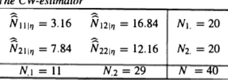
3 while Nu is necessarily larger or equal to nu. The raking ratio estimator does not take into account that the population is finite. In cases with small sample sizes as in this example, this can lead to absurd results. The approximation of the SCW-estimator of the N_hq denoted

N

_hqll/ is given in Table 5.

Table S

The CW-estimator

N111� = 3.16 N121� = 16.84 N1. = 20 N211� = 7.84 N221� = 12.16 N2. = 20

The result is now very coherent. Indeed, N₁�11

=

3.16 is larger that n11.

It thus appears that, in this example at least, the approximation of the SCW-estimator gives a more coherent result than the raking ratio estimator. As for the raking ratio estimator, it seems impossible to give an exact expression for the variance or MS E of the estimator. The following example is the comparison of the mean square error (M SE) for a simple example.

EXAMPLE 4: A simple random sample of 'iize n

=

8 was drawn without replacement from a population of size N

=

12. We examined ail thl- 2 x 2 population contingency tables with non-null cells. For each table, ail the possible sample contingency tables with non-null cells were computed with their probabilities of being selected. Both estimators were computed: the SCW-estimator N 111� and the raking ratio estimator

N

11RR· Next, the exact expectations and mean square errors of these estimators were computed in the following way

E1

=

E[Nu1�lnhq > O,h

=

1,2,q

=

1,2], E2

=

E[NuRRlnhq > 0, h

=

l, 2, q

=

l, 2],

�

2

MSE1

=

E[(Nu1� - N11) lnhq > 0, h

=

l, 2, q

=

l, 2],

�

2

MSE2

=

E[(N11RR - Nu) lnhq > 0, h

=

l, 2, q

=

l, 2].

The expectations and mean square errors were calculated conditional on nhq > 0 because the raking ratio estimator does not exist when one of the nhq

=

O. The effect was defined as the ratio of the two MSE.

MSE1

Effect

= -­

MSE2

Finally, we give the chi-square statistic for the population contingency table

Results are given in Table 6.

(

N N

)

2

2_ 2 2 Nhq -�

X

-LL

_{N N}

h=I q=I �

In one case only, the raking ratio estimator (see bold line in Table 6) gives a better result than SCW-estimator. A detailed examination of Table 6 shows that the larger the value of x

2

, the better

the relative precision of the CW-estimator. For small populations and sample sizes, this example shows that it is generally possible to get an estimator which is much more precise than the raking ratio estimator.

4 Regression Estimation and the Use of Auxiliary Information on Means 4.1 Auxiliary Information on Means

Suppose that the known auxiliary information is the population mean

- 1

x=-I:xk. N _kEU

Table 6

Expectation and MSE of CW ( 1) and raking-ratio (2) estimators

N11 N1. N.1 Ei E2 MSE1 MSE2 Effect x2

1 2 2 1.00 0.81 0.00 0.04 0.00 1.92 1 2 3 1.00 0.95 0.00 0.03 0.00 0.80 1 3 3 1.17 1.15 0.09 0.10 0.89 0.15 2 3 3 1.71 1.58 0.14 0.19 0.74 3.70 1 2 4 1.00 1.00 0.00 0.05 0.00 0.30 1 3 4 1.22 1.22 0.13 0.17 0.76 0.00 2 3 4 1.77 1.73 0.12 0.14 0.85 2.00 1 4 4 1.28 1.31 0.19 0.26 0.74 0.19 2 4 4 1.95 1.93 0.20 0.18 1.11 0.75 3 4 4 2.62 2.48 0.18 0.28 0.64 4.69 1 2 5 1.00 1.01 0.00 0.05 0.00 0.07 1 3 5 1.22 1.23 0.13 0.18 0.70 0.11 2 3 5 1.78 1.78 0.12 0.16 0.76 1.03 1 4 5 1.29 1.32 0.19 0.28 0.69 0.69 2 4 5 2.00 2.00 0.23 0.24 0.95 0.17 3 4 5 2.69 2.64 0.18 0.24 0.75 2.74 1 5 5 1.31 1.34 0.19 0.30 0.64 1.66 2 5 5 2.06 2.07 0.29 0.33 0.88 0.01 3 5 5 2.89 2.84 0.26 0.27 0.96 1.19 4 5 5 3.60 3.46 0.18 0.31 0.57 5.18 1 2 6 1.00 1.00 0.00 0.05 0.00 0.00 1 3 6 1.22 1.22 0.12 0.18 0.71 0.44 2 3 6 1.78 1.78 0.12 0.18 0.71 0.44 1 4 6 1.30 1.32 0.19 0.27 0.70 1.50 2 4 6 2.00 2.00 0.23 0.26 0.89 0.00 3 4 6 2.70 2.68 0.19 0.27 0.70 1.50 1 5 6 1.32 1.39 0.18 0.27 0.67 3.09 2 5 6 2.07 2.10 0.29 0.34 0.87 0.34 3 5 6 2.93 2.90- 0.29 0.34 0.87 0.34 4 5 6 3.68 3.61 0.18 0.27 0.67 3.09 1 6 6 1.40 1.55 0.17 0.31 Ù.55 5.33 2 6 6 2.12 2.19 0.27 0.31 0.88 1.33 3 6 6 3.00 3.00 0.35 0.40 0.87 0.00 4 6 6 3.88 3.81 0.27 0.31 0.88 1.33 5 6 6 4.60 4.45 0.17 0.31 0.55 5.33

Consider the rr -estimator of i given by

i

=

_{_!_}

L

X_k

.

N keS Jrk

The aim is to use

i

as an auxiliary statistic to estimate y. Note that the SCW-estimator is given by

Y

�--_!_"�

li - L, . N keS Jrkli

where rr kli

=

E ( h I

i)

.

In order to construct the SCW-estimator, of y, we thus need an approxi­ mation of rrkJi· If the random vector

i

takes the value z, we have by Bayes's theorem that

A A Pr(i=zlkes)

E (h I i = z) = Pr (k ES I i = z) = rrk

(� ) Pr x =z

In order to compute the conditional inclusion probabilities, it is thus necessary to know the probability distribution of i unconditionally and conditionally on the presence of each unit in the sample. Except for some particular cases, this probability distribution is very complex; for this reason we shall construct approximations of the conditional inclusion probabilities. Next, these approximations will be used to construct an approximation of the SCW-estimator.

lt is possible to derive the means and variances of

i

unconditionally and conditionally on the presence of each unit in the sample:

and

(�) 1 "

Xt.Xf. 1 " " Xt.X_m

Vx = Var X = -₂ L.., -- (1 - Jrr.)

+ -

₂ L.., L, -- (rrem - Jre:7rm)

N f.eU 1rt N ieU meU 1rt.1rm m#-f.

1

L L

X_eX_m

( 1rkf.1rkm)

+-

---

1rkfm -

---N2 _{f.eU meU} rrkrrerrm rrk

f.# m#-f. m#-k

where 1rkt.m is the third-order inclusion probability. Note that Vx can also be written

1 Vx

= -

L(ilk - i)xk. N keU (23) (24) (25) (26) (27)

For simple random sampling without replacement, we get n n n-l n n-ln-2 nk = -,nkl = --- andnkl_{N NN-l} m

= ---.

_NN-lN-2 By C24), C25), C26), we get where _ _ N - n xk -i x1k=_x+----, N-l n N-n a2 V ___ _x 2_ -N-ln' NCN - n)C n - 1) _{ 2 Cxk -

x)

2

}

V1k-x a--- CN a--- 2)CN a--- l)n2 x _N - l 2 l"" 2 a_{x= -L..,Cxk-i).} N kEU

4.2 SCW-Estimation and Regression Estimation

C28) C29) C30)

For simple random sampling without replacement, the normality of the mean estimator was proved by Madow C1948) under some conditions and for a large sample size. If we suppose that i has a normal distribution conditionally and unconditionally in the presence on k E S, then

� n Pr Ci) f Ci)

akC i) = -- = --�---_{Nnkli Pr(i I k E S) fkCi)}

where f (.) Cresp. fk(.)) is the density function of a normal variable with mean i Cresp. i1k) and variance Vx Cresp. Vx1k). Thus,

The SCW-estimator is thus defined by

V-,1x 2 exp----cl -x)_2V 2 x Vx-11lk exp- 2V2 cl -x1k)2 ·

xlk

The following result gives an approximation of the SCW-estimator:

C3 l)

RESULT 2: In simple random sampling, if

1

has a normal distribution unconditionally and conditionally on the presence of each unit in the sample, then an approximation of the SCW-estimator of y conditionally to

1

is given by

y

11

=

t

+ ex

-

1)� I:<xk -x)yk + o,,cn-1

), (32)

nax kES

where n x O_,,(n-1) is a quantity that remains bounded in pro bability when n tends to infinity. Proof of Result 2 is given in Appendix 2.

The approximation given in expression (32) is very similar to the regression estimator given by

A A A 1 � A

Y R

=

Yir + (i - i) ... 2 L.,(Xk - X)Yk· _na

x keS (33)

The only difference between the regression estimator and the approximation of the SCW-estimator is the way we estimate a; and

1

Œ:,:y

= -

L(Xk - X)(yk -

y).

N keU Indeed, in (32), the covariance axy is estimated by

1 �

- L.,(Xk - X)Yk_{n keS} while, in (33), it is estimated by

1� A 1� A A

- L.,(Xk - i)yk

= -

L.,(xk - i)(Yk -

y).

n keS n keS

Moreover, estimator (32) uses the population variance a; while estimator (33) uses an estimatorâ; of a;. The SCW-estimator approximation thus needs more complete auxiliary information.

Result 2 is interesting because it shows that the regression estimator can be introduced without using a superpopulation model. Indeed, it is a natural approximation of the SCW-estimator for large sample size. Moreover, Result 2 also shows that, for simple random sampling, the regression estimator leads to valid conditional inference for large sample size. Indeed, from Result 2, it is obvious that it is asymptotically conditionally unbiased.

5 Discussion

As a conditionally unbiased estimator rarely exists, the conditional unbiasedness concept must thus be enlarged to be really operational. A general method to construct a conditionally VCU�estimator with respect !O an auxiliary statistic is given. Nevertheless, this method brings up a new problem: how to choose the statistic r,?

We advocate the choice of the estimator having the smallest unconditional MS E. Note that a CW-estimator does not necessarily have a smaller MS E than the Horvitz-Thompson estimator. If we consider the example developed in Section 3.1, we see that even if ail the conditional inclusion probabilities are strictly positive, the MS E of the CW-estimator can be larger than the MS E of the Horvitz-Thompson estimator. In poststratification also, it is known that when the interest variable is independent of the poststratification variable, it is preferable to use the Horvitz-Thompson estimator. The following result is useful in order to choose the auxiliary statistic. The conditional bias of the Horvitz-Thompson estimator is given by:

B (� 1 ) 1 � ,rklij - ,rkYir Y/ = _N L., Yk

keU ,rk

By expression (5), the SCW-estimator of this bias is given by B1ij

(Y

ir

I

_{ri)= NI LYk}

(_!_ - -

1 ) ·

keS ,rk 1l'kjij

we get the SCW-estimator. Indeed,

=

_{2_}

L

_{Yk -}

_{2_}

_LYk

(_!__ - -

1 ₎

N kES 7rk N kES 7rk 7rkl11

2-

_N

I:

_{kES 7rkl11} _B.__

Thus, the SCW-estimator can be presented as a Horvitz-Thompson estimator to which a conditional unbiasedness correction is applied.

Note that if the conditional bias was known, we should get the following result as seen in Section 1: (34) Expression (34) gives a first indication on the choice of the auxiliary statistic. The auxiliary statistic r, must be chosen in such a way that Var[E(yirlT/)] is as large as possible. The statistics r, and Yir

must thus be very dependent. Nevertheless, another element must be taken into account. In order that the conditional bias should remain small, the conditional inclusion probabilities must be strictly positive. The choice of the auxiliary statistic must thus be made according to two qui te contradictory criteria: r, must be highly dependent on

y

ir but most of the _7rkl'1 must stay strictly positive.

Finally, the conditional inclusion probabilities must be computable. Auxiliary information is thus necessary to calculate the probability distribution of the auxiliary statistic unconditionally and conditionally on the presence of each unit in the sample. Generally, the knowledge of the probability distribution of r, can be derived from the sampling design p(s) and from the vector (x1 ... Xk ... x N). In some cases, as in poststratification, the conditional inclusion probabilities are computable without difficulty. In some other cases, as in the table adjustment problem, the calculus becomes more difficult. In more complex sampling designs, it becomes practically impossible to find the exact value of the conditional inclusion probability.

The complexity of this problem is due to the fact that three variables ( or three groups of variables) interact: the interest variable; the auxiliary variables used a priori (as the stratification variables or the variables used to sample with unequal probabilities); the auxiliary variables used a posteriori (variables used at the estimation stage). The use of an auxiliary variable without any !eference to a model in a complex sampling design, must thus take into account this third-order interaction. For this reason, the computation of the conditional inclusion probabilities becomes very complex. It is possible, however, to give approximations of these inclusion probabilities even for the complex cases. These approximations will be given in a further paper.

Acknowledgements

The author is grateful to Carl Siirndal for helpful comments and suggestions on earlier versions of this manuscript. I also wish to thank an Associate Editor and a Referee, both of whom provided useful comments that have improved this article.

References

Basu, D. (1958). On sampling with and without replacement. Sankhyii, 20, 287-294. Cochran, W.G. ( 1977). Sampling Techniques, 3rd edition, New York: John Wiley.

Doss, D.C., Hartley, H.0. & Somayajulu, G.R. (1979). An exact small sample theory for post stratification. Journal <!f

Statistical Planning and lnference, 3, 235-248.

Durieux, B. & Payen, J.-F. (1976). Ajustement d'une matrice sur ses marges: la méthode ASAM. Annales de l'INSEE, 22-23, ·311-337.

Fienberg, S.E. ( 1970). An iterative procedure for estimation in contingency tables. Annals <!f Mathematical Statistics, 41, 907-917.

Frielander, D. (1961). A technique for estimating a contingency table, given the marginal totals and some supplementary data.

Journal of the Royal Statistical Society, Al24, 412-420.

Froment, R. & Lenclud, B. (1976). Ajustement de tableaux statistiques. Annales de /'INSEE, 22-23, 29-53. Holt, D. & Smith, T.M.F. (1979). Post stratification. Journal <!{the Royal Statistical Society, Al42, 33-46.

Horvitz, D.G. & Thompson, D.J. (1952). A generalization ofsampling without replacement from a finite universe. Journal <!f

the American Statistical Association, 47, 663-685.

Isaki, C.T. & Fuller, W.A. (1982). Survey design under a regression population model. Journal <!f the American Statistical

Association, 77, 89-96.

Ireland, C.T. & Kullback, S. (1968). Contingency tables with given marginais. Biometrika, 55, 179-188. Konijn, H.S. (1973). Statistical Theory <!fsample survey design and analysis, Amsterdam: North-Holland.

Madow, W.G. ( 1948). On the limiting distributions of estimated based on samples from finite universes. AnnaLî <!fMathematical

Statisâcs, 19, 535-545.

Pathak, P.K. (1961). On simple random sampling with replacement. Sankhyii, A24, 415-420.

Raj, D. & Khamis S.D. (1958). Sorne remarks on sampling with replacement. Annals <!fMathematical Statistics, 29, 550-557.

Rao, J.N.K. (1985). Conditional inference in survey sampling. Survey Methodology, 11, 15-31.

Rao, J.N.K. (1994). Estimating totals and distribution fonctions using auxiliary information at the estimation stage. Journal

<!{Official Statistics, 10, 153-165.

Robinson, J. (1987). Conditioning ratio estimates under simple random sampling. Journal <!f"the American Statistical Asso­

ciation, 82, 826-831.

Stephan, F. ( 1942). An iterative method of adjusting sample frequency data tables when expected marginal totals are known.

Annals of Mathematical Statistics, 13, 166-178.

Thionet, P. (1959). L'ajustement des résultats des sondages sur ceux des dénombrements. Revue de flnstitut International de

Statistique, 27, 8-25.

Thionet, P. (1976). Construction et reconstruction de tableaux statistiques. Annales de l'INSEE, 22-23, 5-27.

Appendix 1 : Proof of Result 1

Note that the use of the auxiliary statistic (n1., n.1) leads to the same result as (n1., n2., n.1, n.2) because of the relations n2. = n -n1. and n.2 = n -n.2. If k E Uu, we get

(N)-

1 2 2 (Nh ) Pr(nh_q

=

rh_q, h

=

l, 2, _q

=

1, 2)

=

_n

n n

_r q , h=I q=I hq Pr(nhq

=

rhq, h

=

l, 2, q

=

1, 2 1 k ES)

=

(N -

1)-'

(Nu -

1)

(N12) (N21) (N22) n - 1 ru - 1 r12 r21 r22 Nru

=

_nNu --Pr(nhq

=

rh.q, h

=

1, 2, q

=

1, 2), Pr(n1.

=

r1., n.1

=

r.1)

=

L

Pr(nu

=

z. n12

=

r1. -Z, n21

=

r.1 -.Z, n22

=

n - ri. - r.1

+

z) z

where

L

_{z extends from max(O,} r1. +r.1 -n, Nu -N1. +r.1, Nu -N.1 +rd to min(r1., r.1, Nu, N

-N1. - N.1 + Nu + r1. + r.1 - n). Moreover, Pr(n1. = r1., n.1 = r.1 1 k E S)

=

L

Pr(nu

=

Z, n12

=

r1. -z, n21

=

r.1 -z. n22

=

n -r1. -r.1 + z

I

k E S)

=

-N N

L

zPr(n11

=

z.n12

=

ri. -z. n21

=

r., -z. n22

=

n -r1. -r.1 + z). n 11 z

Since

E(/k

I

n1.

=

r1., n.1

=

r.1)

n Pr(n1.

=

r1., n.1

=

r.,

1

k E S)

=---

_{N Pr(n1. = r1., n.1 = r.1)}

the conditional inclusion probabilities for the units that belong to U11 can be written

"b+

(N ) _ L...,z=b- zl/l(Nu, z)

1r111,, 11 - _b+

Nu Lz=b- 1/l(Nu, z)

where b-, b+_{, and 1/l(Nu, z) are given in (21), (22), and (20).}

Appendix 2 : Proof of Result 2

The following lemmas will be used in the proof of Result 2.

LEMMA 1: _{Ifn = V}x- 11\i1k -i), then Yk

=

O(n-112), where nao (n-a), a < 0, i saquantity tha t remains bounde d when n � O.

Proof By (28) and (29), we get LEMMA2: Proof By (29) and (30), we get LEMMA3: = (N

-

n a;)-'12 x N

-

n Xk -i Yk _{N-ln N-1 n} = [ _{n(N - 1)} N -n ] 112 Xk -i_Œx = O(n-112). Vxlk = l + O

(.!.) .

Vx n = N(n -1) _{(N - 2 )n} { _{l - (N -l)a;} (Xk -i)2

}

= 1--_n 1 { N -2n N(n -1) (Xk -i)_{(N -2)}

+---

_{(N -2) (N -l)a;} 2 } = 1

+

0 (�).

If

Vxlk vx-1 -1 = O(n-1 ), then Vx Vxli = 1

+

O(n-1 ).

The proof is straightforward.

Proof of Result 2

If we define

X

_e =

v;'

12(x - i), Yk = Vx-'1\x1k - i), and

then (31) can be written

(Vxlk)'/2 x: ( Vx ) ck

= -

exp - - - 1 , Vx 2 Vxlk ( Vxlk) 112

1

x:

(Xe

-

nJ2

Vx }

= -

exp -- + ---Vx 2 2Vxlk Vx A

=

ckexp yk--(Yk - 2ic). 2Vxlk

By using a Taylor development for the vector Yk of (37), we get

where ak(X)

=

Ck

(1 -

Yk Vx

t)

_{+ ncr?\} Vxlk R,(yi°>)

=

ck { exp ri°> 2�:lk (yi°> - 2xc)} x Y{ V Vx _{ V Vx ( Yi°> -

X

_e

r -

_{1 } ,} xlk xlk (36) (37) (38)

where ri°_{> is a vector whose elements are included between the correspondent elements of Yk and}

O. By Lemma 1, we directly get rl

=

0 (n-1) and thus R,(yi°_>)

=

_O

p(n-1). On the other hand, we

have by (36), Lemma 2 and Lemma 3 that

Ck

= {

i

+

0Cn-•) )"2 exp

I

i{

X 0Cn-•)}

=

i

+

o,cn-•

). C39)

By (38) and (39), we get

Finally, we get

Résumé

a(x)

=

(1 +

a;'){

1 - yk(l + O(n-1))

X

_e

+

_Op(n-1)}

= {

1 - YkXc

+

Op(n-1)}

= {

1

+

(i - x)Vx-'(i1k - i)

+

Op(n-1)}.

Dans les enquêtes par sondage, une information auxiliaire sur l'ensemble de la population est souvent disponible. Le but de cet article est de développer une méthode qui permet de prendre en compte cette information auxiliaire à l'étape de

l'estimation au moyen d'un ajustement du biais conditionnel. L'idée de base est de tenter de construire un estimateur sans biais conditionnel. Quatre estimateurs ayant un faible biais conditionnel sont proposés. On montre ensuite que beaucoup d'estimateurs présentés dans la littérature dans le cas du plan simple sans remise peuvent être obtenus en utilisant ce principe d'estimation. Les problèmes du sondage aléatoire simple avec remise, de la poststratification, de l'ajustement d'un tableau de contingence de dimension 2 x 2 sont discutés dans le contexte de l'estimation conditionnelle. Finalement on montre que !'estimateur par la régression peut être obtenu en cherchant une approximation de ce principe conditionnel.