Lire la première partie de la thèse

Lire

la première partie

de la thèse

Chapter 6

Supersonic under-expanded dual

stream jet

The nowadays turbofan engines installed in commercial aircrafts have been designed for specific conditions in order to increase the efficiency at cruise taking into account take-off constraints. The secondary stream of a turbofan engine, in general, is either subsonic or fully expanded, and does not present a shock-cell system characteristic of shock-cell noise. However, due to traffic constraints, the flight level at which the pilot could have the ideal atmospheric conditions for the design point of the engine, cannot always be achieved. The atmospheric conditions and the thrust required at that point determines if a system of shock-cells appears. Due to the fact that the exhaust of the combustion chamber goes through the primary stream, its temperature is higher than the one encountered in the secondary stream. For this reason, it is most likely to find the shock-cell system in the secondary stream.

This chapter discusses the results obtained with LES of a dual stream configuration at condi-tions representative of real flight. This case of study has been tested experimentally at the von Karman Institute for Fluid Dynamics in the new Free jet AeroacouSTic laboratory (FAST). First, the definition of the case of study, the characteristics of the mesh and the simulation pa-rameters are described in Sec. 6.1. Next, in Sec. 6.2 a few words are given to the experimental setup against which the numerical results are compared. Then, the analysis of the results are discussed in Sec. 6.3. Finally, a summary and some perspectives are introduced.

A part of the results discussed in this chapter were presented in the 2016 AIAA/CEAS con-ference [205]. Some of the data produced with this case of study was used by other partners of the project AeroTraNet2. More information about the collaborations can be found in Appx. C.

6.1

LES configuration

This section presents the main characteristics of the large eddy simulation of a dual stream jet. The characteristics of the code used for the LES are explained in Ch. 2. In addition, the LES procedure and mesh generation are extensively described in Ch. 3.

6.1.1 Case conditions

The case of study is a coaxial jet where the primary flow is cold and subsonic with an exit Mach number of Mp = 0.89 (CNP R = 1.675) and the secondary stream is operated at supersonic under-expanded conditions with a perfectly expanded exit Mach number of Ms = 1.20 (F NP R = 2.45). Here, CNP R and F NP R stand for Core and Fan Nozzle to Pressure Ratio respectively (see Ch. 1 for a wider explanation of the NPR). The jets are established from two concentric convergent nozzles with primary and secondary diameters of Dp = 23.4 mm and Ds= 55.0 mm respectively. The thicknesses of the nozzles at the exit are of 0.3 mm. The Reynolds numbers based on the exit diameters and the perfectly expanded conditions are

Rejp= I ρjUjD µj J p = 0.67 × 106_{, (6.1)} and Rejs= I ρjUjD µj J s = 2.64 × 106_{, (6.2)}

where the subscript {•}j refers to the perfectly expanded conditions, and the subscript {•}p and {•}s refer to the primary and secondary streams respectively. The ambient conditions used for this case of study are a pressure p∞ = 101, 325 Pa and a temperature T∞ = 283 K.

The generating pressure or total pressure is ptp = 1.6972 × 105 Pa for the primary stream and

pts = 2.4825 × 105 Pa for the secondary stream. The total temperature Tt is set equal to the ambient temperature T∞ for both streams.

A supersonic under-expanded jet expands to the ambient pressure by means of the so-called shock-cell system. Its subsonic counterpart matches the nozzle exit pressure with the local static pressure found outside the nozzle without the need of an expansion fan. The three-dimensional effects of the secondary stream and the shape of the nozzle can modify the local pressure in its vicinity. When the local static pressure is modified with respect to the room static pressure the jet actually expands to the new static pressure, modifying the local nozzle to pressure ratio. In this study, the regular definition of NPR for the primary jet is kept, i.e. with respect to the room static pressure and not the local static pressure.

The main conditions are summarized in table 6.1.

D [mm] Mj N P R pt [Pa] Tt [K] Rej

Primary 23.4 0.89 1.675 _{1.6972 × 10}5 _{283 0.67 × 10}6

Secondary 55 1.20 2.45 _{2.4825 × 10}5 _{283 2.64 × 10}6

Table 6.1: Conditions for the primary and secondary nozzles.

6.1.2 Mesh definition

The structured multi-block mesh used for the LES is defined in this section. The mesh contains 200 × 106 _{cells. Figure 6.1 (a) displays a gridplane of the mesh at z/D}

s= 0 where the interior of the pink region represents the physical domain. The region outside the pink region defines

x/D

y

/D

0

5

10

15

20

-5

0

5

A

B

C

D

E

Figure 6.1: Mesh grid planes representing every fourth nodes in the plane z/Ds= 0 for (a) a

general view and (b) a closer look at the nozzle exit. (c) shows the exit plane of the nozzle. The capital letters [A, E] illustrate different sections of the mesh.

the singularity at the axis. The capital letters [A, . . . , E] depicted in Figure 6.1 (b) illustrate different sections of the mesh. Section A is situated forward to the primary nozzle exit plane. Section B considers the region between the exit of the primary and secondary nozzle. Section C is located over the secondary nozzle and sections D and E, define the interior of the primary (D) and secondary (E) nozzles respectively. The lips of both nozzles are discretized with 6 cells. The axial gridplane situated at the exit of the primary nozzle is shown in Fig. 6.1 (c). Table 6.2 summarizes the mesh distributions in each section.

A B C D E

Axial 1, 132 108 172 100 110

Radial 600 490 326 100 162

Azimuthal 256 256 256 256 256

Table 6.2: Mesh distribution in each section for the axial, the radial and the azimuthal direc-tions.

The walls of the internal sections of the nozzles (section D and E) as well as the external section of the primary nozzle (section B) attain a resolution at the wall of y+ _{≈ 15 with 20}

points in the boundary layers. The maximum expansion ratio between adjacent cells achieved in the mesh is not greater than 4%. The radial discretization at different axial positions is shown in Fig. 6.2 (a).

0 5 10 15 20 25 −4 −3 −2 −1 0 1 2 3 4 dr/D s x10 3 r/D_s 0.5D_s 2D_s 4D_s 6D_s 8D_s 10D_s (a) 0 5 10 15 20 25 0 2 4 6 8 10 12 14 1 23 4 5 6 dx/D s x10 3 x/D_s x−axis (b)

Figure 6.2: Discretization of the mesh along (a) the radial distribution for different x/Ds and

(b)the axial distribution along the axis, where dr is the radial step and dx the streamwise one.

The maximum Helmholtz number (Hes= fDs/a∞) that the mesh is able to capture at the end

of the physical domain is about 4. The radial domain size grows with the axial position in order to take into account the expansion of the jet (from r/Ds= 2.5 at the exit of the primary nozzle to r/Ds = 5 at x/Ds = 13), nonetheless, the maximum Hes number is kept constant at the boundary with the sponge layer. The axial discretization shown in Fig. 6.2 (b) is composed of 6 sections defined by the enumerated symbols. In the interior of the primary nozzle, segments 1 2 and 2 3, the mesh is refined where the vortex-ring is located (point 2). At this position,

vortex-ring used to transition to turbulence. At the exit of the primary nozzle (point 3), the aspect ratio of the cells at the wall attains a value of 4. In the third segment 3 4, the mesh elongates at a rate of 3%. This stretching allows for a drastic reduction of the total amount of cells in the axial direction. The segment 4 5 consists in a uniform discretization. Then, in segment 5 6, the mesh is slowly elongated up to a mesh size able to capture a Helmholtz number of 4. The last section, starting at point 6, is the one corresponding to the sponge layer where the mesh has a stretching ratio of 10%.

6.1.3 Simulation parameters

The numerical computation is initialized by a Reynolds-Averaged Navier-Stokes (RANS) sim-ulation using the Spalart-Allmaras turbulence model [169] as explained in Sec. 3.2. The RANS solution is fully wall-resolved in the internal and external sections of the nozzles with a maxi-mum wall unit (y+_{) of unity with 30 points in the boundary layer. The nozzle is modeled in}

the interior up to 10 primary diameters and the RANS domain extends to 50 primary diame-ters in the radial and axial directions. The LES is then initialized from the RANS simulation keeping the inlet profiles. In order to accelerate the initialization from a steady state to a temporal resolved state, an intermediate coarse mesh of 25 × 106 _{cells is considered. The flow}

is initialized over 90 dimensionless convective times (ˆtp = ta∞/Dp) and then the data are interpolated over the fine mesh explained in Sec. 6.1.2. Before the flow could be considered as initialized, 60 additional dimensionless convective times are computed with the fine mesh to evacuate interpolation errors and let the flow adapt to the fine mesh. The final computation is then run for 186 dimensionless convective times to obtain the statistics. The simulation time corresponds to 80 dimensionless convective times with respect to the secondary diameter Ds. As it is described in Sec. 6.3, the secondary stream presents an oblique shock at the axial position of the exit plane of the primary nozzle. After 186 ˆtp some instabilities occurred near the oblique shock which forced us to stop the LES. Due to the small computational time and in order to increase the convergence of the results, some of them are averaged in the azimuthal direction. A dimensionless time step of 0.00027 equivalent to a CFL about 0.9 was selected for the data extraction phase. In dimensional quantities, the time step is equivalent to 0.0187 µs.

The boundary conditions used in the simulation are sketched in Fig. 6.3 (a). Non-reflective boundary conditions of Tam and Dong [160] extended to three dimensions by Bogey and Bailly [161] are set at the inlets as well as at the lateral boundaries. The exit boundary condition is based on the characteristic formulation of Poinsot and Lele [158]. Additionally, sponge layers are employed around the domain to attenuate exiting vorticity waves. An inflow forcing based on the vortex-ring of Bogey and Bailly [73] is applied in the interior of the subsonic nozzle to help transition to turbulence as shown in Fig. 6.3 (b) but not in the interior of the secondary supersonic nozzle. In order to accurately define the vortex-ring and maintain the levels of turbulence throughout the convergent secondary nozzle, a much finer discretization and longer interior section would have been needed. This would have increased the cost of the computation, without assuring the correct (at the moment unknown) turbulent levels. Last, no-slip adiabatic wall conditions are set at all the wall boundaries of the nozzles. No wall turbulence models are used.

that an oblique shock appears at the end of the primary nozzle in the secondary stream as it is later described in Sec. 6.3.1. Although the shock-limiting technique was active, the flow became unstable near the oblique shock. This computation was run with the spatial filter explained in Sec. 2.2.2 of order 6.

In terms of computing cost, the LES was run on 1024 processors using HPC resources from GENCI-OCCIGEN [CCRT/CINES/IDRIS] (Grant 2016-[x20162a6074]). The total computa-tional time was about 1, 750, 000 CPU h, which counts for the RANS used to initialize the LES, the computation on the coarse mesh, the adaptation phase from the coarse mesh to the fine mesh, and the actual LES of 80 convective times.

sponge!layer non-reflective!radiative!conditions! NSCBC farthest!FW-H!surface 37.5!Dp,!!15.95!Ds 30!Dp,!12.7!Ds 26!Dp, 11.1!Ds 16!Dp, !!7!Ds (a) vortex-ring!forcing 0.75!Dp,!0.32!Ds 0.25!D_p,!1.06!D_s 3.77!Dp,!1.6!Ds 0.25!Dp,!1.06!D!s (b)

Figure 6.3: Sketch of the numerical and physical domain in (a) a general view and (b) a detailed view.

6.1.4 Data extraction

The data extracted are divided in mean, cuts, numerical probes and topological surfaces. The cuts and topological surfaces were saved every 400 iterations which is equivalent to a frequency of 133.45 kHz. On the other hand, the numerical probes were extracted every 100 iterations or 533.78 kHz.

The mean flow was averaged azimuthally to increase the convergence. Due to the reduced simulated physical time, the second order moments are not fully converged, notably in the downstream regions where the large structures are developed. Therefore, an interpolation into a polar mesh was performed in order to facilitate the azimuthal average. The average of second order moments was done following a prior change of variables at each azimuthal position as formulated in Appx. A.

Plane cuts were extracted at z/Dp = 0, and at the axial locations x/Dp ∈ {0, 5, 10}. Three sets of probes were extracted in this simulation sharing the same axial discretization. In the range −0.9 < x/Dp < 15 the data were extracted every 0.1 Dp. Farther downstream, in the range 15 < x/Dp < 25 the data were extracted every 1 Dp. The different data sets are: a set of probes at the axis (referred to as AXIS), a set at the shear-layer between the primary and the secondary stream (referred to as LIP P), a set at the secondary shear-layer (referred to as LIP S), and three sets situated in the near-field with an expansion angle of 8 degrees from

sets but the one located at the axis are composed of 16 azimuthally distributed probes. The far-field sound is obtained by means of the Ffowcs-Williams and Hawkings analogy (FWH) [196]. The surfaces used to extrapolate the variables to the far-field are located in three concentric topological surfaces starting at r/Dp = {3, 4, 5} from the axis and growing with the mesh. The surfaces are closed on the exterior of the secondary nozzle and open at the outlet. The cut-off mesh Strouhal number is Sts = fDs/Ujs ≈ 6.0. The sampling frequency was set to 65 kHz which gives a sampling Strouhal number higher than the mesh cut-off limit. The noise is propagated up to a distance of 30 Ds which is far enough to be considered as proper far-field according to Viswanathan [57].

6.2

Experimental setup

In this chapter, the numerical results are compared to the experimental data obtained at the von Karman Institute for Fluid Dynamics (VKI) by its researchers and other partners of the same European project AeroTraNet2, framework of this thesis. The facility named FAST (Free jet AeroacouSTic laboratory) was built between 2013 and 2016 and it has been specially designed for coaxial jets [206, 198] even though it can also be run for single jets. The nominal testing conditions of the facility are for the core stream 1.35 < CNP R < 1.72 and for the fan stream 2.00 < F NP R < 2.50. Unfortunately, as a result of several delays in the manufacturing process of some parts of the experimental facility, the CFD was carried out before the experimental campaign. This has led to some geometrical differences that are summarized in the following.

The Computer Assisted Design (CAD) of the final coaxial nozzle installed at VKI is shown in Fig. 6.4 (a). The screws used to attach the nozzle to the ducts are not modeled in the current study as seen in Fig. 6.4 (b). After discussion with the experts at VKI, the effect of the screws was assumed to be negligible and thus, it was not modeled in the RANS simulation nor were considered for the LES domain as illustrated in Fig. 6.4 (b). Moreover, due to some pressure losses in the feeding pipeline of the experimental facility, the target conditions where not possible to reach with the original nozzle diameters presented in Table 6.1. Therefore, a new nozzle was machined with reduced dimensions by 20%. Since the numerical campaign started before the experimental one, the modeled nozzle in this work has the original dimensions. The different dimensions have an impact on the Rej, the development of the internal boundary layers, and the acoustics. In addition, it was later found that when the air flow was active in the experiments, the secondary nozzle moved vertically about 2 mm (or 0.05 Ds) in the jet direction. The researchers at VKI believe that this could be due to the vertical strain of the external ducts when the pressurization is active.

Two sets of data are compared in this chapter, pressure probes situated in the far-field and the field obtained by Particle Image Velocimetry (PIV). The polar antenna was placed at a distance equal to 30 Dsset with a frequency sampling of 250 kHz, which corresponds to about 224 _{samples (67 seconds). The PIV was captured with two cameras set in parallel with a small}

overlapped region. The images were captured with a resolution of 2, 360 × 1, 766 pixels2 _and

a sampling frequency of 15 Hz. The experiments were run in five realizations of 40 seconds, generating 600 images per run. Two experiments were done with the same conditions but with a different location of the cameras in order to generate an extended view of the flow

(a)

RANS

LES

(b)

Figure 6.4: (a) CAD drawing of the manufactured coaxial nozzle. (b) Modeled nozzle for the RANS simulations and LES. Courtesy of D. Guariglia [198].

downstream. With a 50% overlap of the windows a resolution of 393 × 294 vectors is imposed. The final image, with the 4 nested frames as shown in Fig. 6.5 is composed of 393 × 1085 vectors.

6.3

Analysis of results

6.3.1 Aerodynamic field

Comparisons with experimental PIV

In this section, the main aerodynamic flow features of the LES are compared with the experi-mental PIV fields from VKI. The contour plots investigated in this section, are divided in a top part where the experimental PIV results are displayed, and a bottom part with the numerical PIV. The sign of the vertical velocity is inverted on the numerical contours in order to have the same color scheme. The Mach number isolines with levels M = {0.9, 1.0, 1.1, 1.2, 1.3, 1.4} are shown on all contours plots in solid black line. In addition, the data contained over some vertical lines are extracted at the starting and middle point of the last 7 recognizable shock-cells. The extracted profiles are depicted in a separate figure where the top represents the line crossing the starting point of a shock-cell and the bottom, the middle point. Due to differences in shock-cell size and location between the experimental and the numerical fields, the extracted lines are grouped by shock-cell number. The comparable average quantities of interest that were computed with the PIV are: Mach number, axial velocity u, radial velocity vr, variance of the axial velocity u′ 2_{, variance of the radial velocity v}′ 2 _{and the variance of the product}

Figure 6.5: Instantaneous PIV velocity flow field with Mach number M = 1 isolines for the conditions CNP R = 1.675 and F NP R = 2.500. Courtesy of D. Guariglia.

absolute velocity (assuming w = 0) from the PIV, using the isentropic relation M = ö õ õ õ ô u2_{+ v}2 γRTt− (u2+ v2)(γ − 1)₂ , (6.3)

where Tt is the total temperature taken as 283 K.

The Mach number contours are shown in Fig. 6.6. The primary subsonic jet is enclosed by a supersonic under-expanded annular jet. It creates the primary potential core surrounded by an annular potential core where the shock-cells live. These concentric potential cores merge further downstream. The supersonic under-expanded secondary flow undergoes the birth of an oblique shock at the exit of the primary nozzle due to the difference in slope between the internal section of the primary nozzle and the outer section of the nozzle. This oblique shock theoretically generates a secondary shock-cell system that coexists with the one generated by the under-expanded supersonic jet at the exit of the secondary nozzle even though is not clearly visible in Fig. 6.6. Due to the oblique shock, and the shock-cell system that appears in the secondary stream, the actual Mach number obtained at the exit of the primary nozzle achieves a value of 0.51 instead of the design value of 0.89. Nonetheless, the design value is reached after an axial distance of 1 Dp. Moreover, the shock-cells of the secondary stream modify the Mach number and the pressure in the primary stream.

The shock-cell lengths measured with the Mach number oscillations in the axis of the primary jet are shown in Table 6.3. Due to a different development of the jet, and the displacement of the experimental secondary nozzle, the last shock-cell differs in position about 0.62 Ds. The shock-cell lengths are smaller in the numerical simulation with a reduction between 10% in the first measured shock-cells to up to 20% in the last ones. This remarkably difference has an impact on the shock-cell noise main frequencies. Because the shock-cell distribution changes, the data from particular lines were extracted at the locations relative to each shock-cell as it is illustrated in Fig. 6.7 for the Mach number. Regardless of the differences in position, and shock-cell length, the extracted LES data of each line have good agreement with the experimental Mach number profiles at all relative positions. The peaks at the center of the secondary stream and the values at the axis of the primary stream have the same values. The

main discrepancy comes from the shape of the shear-layer, being about 40% wider in the LES. This difference in the shear-layer thickness is responsible for the difference in shock-cell length. The compression wave that is reflected in the shear-layer will occur closer to the axis if the shear-layer is wider. Due to the geometry of the shock-cells, the smaller the shock-cells are in the vertical direction, the smaller they are in the axial direction. The difference in the thickness of the shear-layer can be a matter of a bad discretization of the shear-layer which could increase the dissipation on that region or/and by a difference in the initial turbulence levels.

L2_sh/Ds L3_sh/Ds N P R L_sh4 /DsL5_sh/Ds L6_sh/Ds

PIV 0.476 0.473 0.486 0.455 0.420

LES 0.425 0.400 0.390 0.365 0.340

%decrease 10.78 15.40 19.67 19.69 19.04

Table 6.3: Shock-cell length obtained with the PIV and LES measured at the axis of the primary stream.

Figure 6.6: Mach number contours of the mean field from PIV (top) and LES (bottom). The black solid lines represent the Mach number from 0.9 to 1.4 with an interval of 0.1.

The radial velocity vr contours are displayed in Fig. 6.8 and the extracted vertical lines in Fig. 6.9. The axial velocity exhibits a similar pattern than the Mach number and is not presented. On the other hand, the vertical velocity shows a very distinguished pattern in the boundaries of the shock-cells, classical of expanded jets. As it happens for an under-expanded single jet as explained in Ch. 5, the expansion fan generated at the lip of the nozzle bounces back to the jet as a compression wave. The jet expands radially in the expansion zones whereas it comes back to the center in the compression zones. Between each different region, compression-expansion or expansion-compression, there is a neutral zone where the jet changes the sign of the second axial derivative of the pressure. In other words, there is a maximum and a minimum in the pressure (and other variables such as Mach number and axial velocity). On the other hand, at these locations, the radial velocity changes the sign

1.0 0.5 R_p/D_s 0.0 R_p/D_s 0.5 1.0 0.0 0.0 0.0 0.0 0.0 0.0 0.0 0.0 0.0 0.0 0.0 0.0 0.0 0.0 0.0 0.0 r/D s M num. elsA exp. VKI #1 #2 #3 #4 #5 #6 #7 #1 #2 #3 #4 #5 #6 #7 Shock−cell Center 1 Shock−cell Edge

Figure 6.7: Mach number profiles of the mean field from PIV (dashed) and LES (solid). The top part corresponds to axial positions at the center of a shock-cell and the bottom part to axial positions at the edge of a shock-cell.

from negative to positive values otherwise. Differently to the single jet, here, the expansion occurs only from the lip of the secondary nozzle and it bounces back as a compression wave on the shear-layer of the primary jet instead of on the symmetry axis. Figure 6.8 displays the expansion fans and compression waves on the secondary stream with a triangular shape. Figure 6.9 (a) shows the velocity profiles in the neutral zones of the jet. As it can be seen, the different profiles have the same shape independently from the axial location and independently of whether they are located after the expansion zone or after the compression zone. The experimental results exhibit less smooth profiles than the numerical ones due to the fact that only 3000 snapshots were averaged in the PIV against the average of 679, 200 iterations for the LES. As it can be seen, the position of the peaks are well captured even though they are smoother in the simulation. Regardless of the amplitude of the peaks, on one hand, the profiles have good agreement in the downstream positions. On the other hand, the negative radial velocity caused by the suction of the jet outside the shear-layer is higher in the LES. This might be because the modeled nozzle is bigger than the experimental one or by some installation effects. A peak of radial velocity is achieved in the shear-layer generated by the expansion of the jet. Moreover, a smaller negative peak is found in the shear-layer between the primary and the secondary jet. At this location, it is negative because the secondary stream expands on to the primary stream. At the axis, the mean radial velocity should be zero. This is confirmed by the LES, however, the experimental results present a slight positive value in the first shock-cells. At the time of writing of this manuscript, three possible hypothesis were shared by private communications with D. Guariglia at VKI: the laser sheet could be not perfectly centered at the axis, there is a misalignment of the axis direction of the primary nozzle, or last, the PIV is biased by the uncertainty of an average over only 3000 images. The profiles of some of the shock-cells in the compression and expansion zones are shown in Fig. 6.9 (b). The suction differs about 50% close to the nozzle exit but this difference is reduced further downstream. In the expansion zone, the flow expands and tends to go away from the axis which is represented by a positive radial velocity. The effect of the expansion can be seen as an extra peak which is overlapped with the peak of the expansion of the jet. The two peaks can be slightly recognized in the first shock cell as a change of curvature. In addition, in the compression zone, there is a positive peak that is developed from the expansion of the

(a)

Figure 6.8: (a) Radial velocity vrcontours of the mean field from PIV (top) and LES (bottom).

The black solid lines represent the Mach number from 0.9 to 1.4 with an interval of 0.1. jet followed by the negative peak of the compression zone. The peak related to the expansion or compression has an opposite influence over the primary jet, as it is demonstrated by the peaks close to the axis. Overall, good agreement with the experiments is obtained.

The contours of the second order central moments of the axial u′ 2_{and radial velocity v}′

r 2 are

computed and shown in Fig. 6.10. As it was presented in Fig. 6.9, here, the higher expansion ratio of the jet is noticeably closer to the nozzle exit but it achieves the same width at the end of the potential core. Figure 6.11 illustrates quantitatively the difference on the extracted lines. At first glance, both the axial and the radial velocity variances present higher levels close to the nozzle exit for the numerical results. This can be expected from a bad resolution of the PIV [207, 208] in the thinner regions of the shear-layers. Moreover, further downstream, the axial velocity variance increases for the experiments in the secondary shear-layer. However, the simulation captures well the peak in the primary shear-layer in the first shock-cells and shows a slight reduction in the last ones for the axial velocity. The peaks are encountered at the same radial positions.

Next, the Reynolds stress expressed by the cross-term u′_v′

r displayed in Fig. 6.12 is analyzed. Figure 6.12 (a) focuses on the secondary shear-layer whereas Fig. 6.12 (b) is saturated in order to focus on the primary shear-layer. Similarly to the variance of the axial and radial velocity, the cross-term presents a higher intensity closer to the nozzle for the LES whereas farther downstream it is dissipated. The primary shear-layer shows high-level spots at the edge of the shock-cells. As shown in Fig. 6.13, the cross-term u′_v′

r computed for the LES is twice the amount of the experimental results. Further downstream the levels are similar.

Length-scales analysis

The length-scales and time-scales for the axial (L(1)₁₁) and radial velocity (L(1)₂₂) are shown in Fig. 6.14 and Fig. 6.15 respectively. They are computed along the axis, the primary lip-line and the secondary lip-line and compared to those of Laurence [209] and Davies et al. [210].

1.0 0.5 R_p/D_s 0.0 R_p/D_s 0.5 1.0 0.0 0.0 0.0 0.0 0.0 0.0 0.0 0.0 0.0 0.0 0.0 0.0 0.0 0.0 0.0 0.0 r/D s v − /v−_max num. elsA exp. VKI #1 #3 #5 #7 #1 #3 #5 #7 Shock−cell Center 1 Shock−cell Edge v−_max = 7 m/s (a) 1.0 0.5 R_p/D_s 0.0 R_p/D_s 0.5 1.0 0.0 0.0 0.0 0.0 0.0 0.0 0.0 0.0 0.0 0.0 0.0 0.0 0.0 0.0 0.0 0.0 r/D s v − /v−_max num. elsA exp. VKI #1 #2 #3 #5 #1 #2 #3 #5 Expansion Zone 1 Compression Zone v−_max = 7 m/s (b)

Figure 6.9: (a,b) Radial velocity vr profiles of the mean field from PIV (dashed) and LES

(solid). For (b), the top part corresponds to axial positions at the center of a shock-cell and the bottom part to axial positions at the edge of a shock-cell. For (b), the top part corresponds to axial positions in the expansion zone of a shock-cell and the bottom part to axial positions in the compression zone of a shock-cell. In this figure, some of the shock-cells are omitted for clarity.

(a)

(b)

Figure 6.10: (a) Variance of the axial velocity u′ 2 _{and (b) radial velocity v}′

r 2 contours of

the mean field from PIV (top) and LES (bottom). The black solid lines represent the Mach number from 0.9 to 1.4 with an interval of 0.1.

1.0 0.5 R_p/D_s 0.0 R_p/D_s 0.5 1.0 0.0 0.0 0.0 0.0 0.0 0.0 0.0 0.0 0.0 0.0 0.0 0.0 0.0 0.0 0.0 0.0 r/D s u − ’ − u − ’ − /u−−’u−−’_max num. elsA exp. VKI #1 #2 #3 #4 #5 #6 #7 #1 #2 #3 #4 #5 #6 #7 Shock−cell Center 1 Shock−cell Edge u − ’ − u − ’ − max = 4000 (m/s) 2 (a) 1.0 0.5 R_p/D_s 0.0 R_p/D_s 0.5 1.0 0.0 0.0 0.0 0.0 0.0 0.0 0.0 0.0 0.0 0.0 0.0 0.0 0.0 0.0 0.0 0.0 r/D s v − ’ − v − ’ − /v−−’v−−’_max num. elsA exp. VKI #1 #2 #3 #4 #5 #6 #7 #1 #2 #3 #4 #5 #6 #7 Shock−cell Center 1 Shock−cell Edge v − ’ − v − ’ − max = 2000 (m/s)2 (b)

Figure 6.11: (a) Variance of the axial velocity u′ 2 _{and (b) radial velocity v}′

r2 profiles of the

mean field from PIV (dashed) and LES (solid). The top part corresponds to axial positions at the center of a shock-cell and the bottom part to axial positions at the edge of a shock-cell.

(a)

(b)

Figure 6.12: Variance of the product of the axial and radial velocities u′_v′

r contours of the mean

field from PIV (top) and LES (bottom). (a) General view. (b) Zoomed view with saturated contours. The black solid lines represent the Mach number from 0.9 to 1.4 with an interval of 0.1. 1.0 0.5 R_p/D_s 0.0 R_p/D_s 0.5 1.0 0.0 0.0 0.0 0.0 0.0 0.0 0.0 0.0 0.0 0.0 0.0 0.0 0.0 0.0 0.0 0.0 r/D s u − ’ − v − ’ − /u−−’v−−’_max num. elsA exp. VKI #1 #2 #3 #4 #5 #6 #7 #1 #2 #3 #4 #5 #6 #7 Shock−cell Center 1 Shock−cell Edge u − ’ − v − ’ − max = 1500 (m/s)2

Figure 6.13: Variance of the product of the axial and radial velocities u′_v′

r profiles of the mean

field from PIV (dashed) and LES (solid). The top part corresponds to axial positions at the center of a shock-cell and the bottom part to axial positions at the edge of a shock-cell.

auto-correlation up to the first minima. The length-scales of the axial velocity have good agreement with the experimental fit for both the primary and secondary lip-lines as displayed in Fig. 6.14 (a). The length-scales at the axis overcome a maxima at the position of the shock-cells that oscillates with them. Then, it decreases due to the increase in axial velocity related to the mixing of the secondary supersonic jet. Finally it increases again and recovers the same length-scales as the other references. A similar effect can be encountered at the primary lip-line where two slopes are clearly differentiated before and after the merging with the secondary stream. As expected, the length-scales of the radial velocity shown in Fig. 6.14 (b) are lower to those computed for the axial velocity. The time-scales of the axial velocity presented in Fig. 6.15 (a) exhibit an increase at two different rates, one before the merging of the potential cores and one afterwards. The maxima observed at the axis (Fig. 6.14 (a)) is smoothed into a plateau for the timescale. On the other hand, the time-scales of the radial velocity converge into the same time-scales independently of the radial position as displayed in Fig. 6.15 (b).

!0 !0.2 !0.4 !0.6 !0.8 !1 !0 !2 !4 !6 !8 !10 L11 (1) /!D s x/D_s Axis Lipline!Primary Lipline!Secondary Liepman! Laufer (a) !0 !0.2 !0.4 !0.6 !0.8 !1 !0 !2 !4 !6 !8 !10 L22 (1) /!D s x/D_s Axis Lipline!Primary Lipline!Secondary (b)

Figure 6.14: Lengthscale of (a) the axial velocity u and (b) the radial velocity vr along the

axis, the lip-line of the primary nozzle and the lip-line of the secondary nozzle.

!0 !0.2 !0.4 !0.6 !0.8 !1 !0 !2 !4 !6 !8 !10 T11 (1) !U s !/!D s x/D_s Axis Lipline!Primary Lipline!Secondary (a) !0 !0.2 !0.4 !0.6 !0.8 !1 !0 !2 !4 !6 !8 !10 T22 (1) !U s !/!D s x/D_s Axis Lipline!Primary Lipline!Secondary (b)

Figure 6.15: Timescale of (a) the axial velocity u and (b) the radial velocity vr along the axis,

Impact of a shifted nozzle

As it was mentioned in Sec. 6.2, the experimental secondary nozzle suffered from a slight axial shift when the flow was active. Unfortunately, this effect was reported after the large eddy simulation was carried out. In this section, a RANS computation of the shifted nozzle is compared to the original one used to initialize the LES in order to quantitatively measure the impact on the shock-cell development. A positive axial shift of 0.05 Ds was considered. Due to the shape of the primary nozzle, the shift of the secondary nozzle increases the effective area of the secondary stream by 5% from A/D2

s = 47.63 to A/D2s = 50.05. This increase in area implies that the mass flow rate also increases 5% with respect to the original position of the nozzle (see Eq. (1.24)). On the other hand, the shift does not affect the FNPR because as shown in Eq. (1.25) it is determined by the total and the ambient pressure.

The Mach number contours are compared in Fig. 6.16. The Mach number at the primary axis and at the skewed secondary axis are displayed in Fig. 6.17 and 6.18 respectively. The general view of Fig. 6.16 (a) shows that the pattern of the shock-cells is similar but shifted to the right which is also visible as an extension of the Mach number lines in the potential core. A close-up look of the nozzle exit (Fig. 6.16 (b)) displays that the first shock-cell is intersected by the oblique shock that appears at the exit of the primary nozzle. Due to this intersection, the pressure is higher closer to the oblique shock in the shifted configuration which makes the Mach number jump increase astonishingly by 48%. The original nozzle has a Mach number jump from Ml= 1.165 to Mr= 0.99 (where the subscripts {•}l and {•}r stand for conditions at the left and right sides of the shock). The shifted nozzle has a Mach number jump from Ml = 1.19 to Mr = 0.93. This higher intensity is perceived by the subsonic primary jet as shown in Fig. 6.17. The amplitude of the Mach number variations in the primary jet increases and is also shifted. This effect is less prominent in the secondary stream as displayed in Fig. 6.18. The shock-cell length is measured in the primary axis in order to avoid topological differences between both nozzles. They are presented in Table 6.4. The variation in shock-cell length is of less than 4% and identical for some shock-cells.

L1_sh/Ds L2_sh/Ds L_sh3 /Ds L4_sh/Ds L5_sh/Ds

Modeled 0.408 0.408 0.396 0.357 0.345

Shifted 0.421 0.408 0.408 0.370 0.345

%increase 3.12 0 3.22 3.57 0

Table 6.4: RANS shock-cell length for the modeled and the shifted nozzle measured at the axis of the primary stream.

In summary, the shift of the nozzle increases the mass flow rate of the secondary stream, it increases the intensity of the oblique shock and the Mach number variations in the primary stream and slightly increases the shock-cells length. All these changes could have an impact on the acoustics, for example: the reinforced oblique shock could modify the behavior of the tonal noise screech or the change in the Mach number in the primary stream could affect the development of the internal shear-layer. Nonetheless, the actual impact of this displacement on the acoustics remains uncertain and should be further studied experimentally and numerically

(a)

(b)

Figure 6.16: Mach number contours for the (a) LES mean (top) and RANS (bottom) simula-tions. (a) General view. (b) Zoomed view.

!0.8 !0.82 !0.84 !0.86 !0.88 !0.9 !0.92 !0.94 !0 !2 !4 !6 !8 !10 M y/D_s DESIGN!!NOZZLE SHIFTED!NOZZLE (a) !0.86 !0.87 !0.88 !0.89 !0.9 !0.91 !0.92 !0.5 !1 !1.5 !2 !2.5 !3 M y/D_s DESIGN!!NOZZLE SHIFTED!NOZZLE (b)

Figure 6.17: Comparison of the Mach number profiles along the axis of the primary nozzle between the modeled nozzle and the manufactured one. (a) General view. (b) Zoomed view.

!0.7 !0.8 !0.9 !1 !1.1 !1.2 !1.3 !0 !2 !4 !6 !8 !10 M y/D_s DESIGN!!NOZZLE SHIFTED!NOZZLE (a) !1.1 !1.12 !1.14 !1.16 !1.18 !1.2 !1.22 !1.24 !0.5 !1 !1.5 !2 !2.5 !3 M y/D_s DESIGN!!NOZZLE SHIFTED!NOZZLE (b)

Figure 6.18: Comparison of the Mach number profiles along the skewed secondary potential core between the modeled nozzle and the manufactured one. (a) General view. (b) Zoomed view.

6.3.2 Acoustic-hydrodynamic filtering in the near-field

The near-field flow is composed of hydrodynamic and acoustic perturbations. In order to focus the study in either one or the other, the acoustic-hydrodynamic filtering [181] is applied to the dual stream jet. This procedure was successfully applied to the supersonic under-expanded single jet in Sec. 5.3.2 and it is explained in detail in Sec. 3.3.2. The filtering is carried out on the probes located in the near-field at r = {0.85Ds, 1.7Ds} at the secondary nozzle exit plane with an expansion angle of 8◦_.

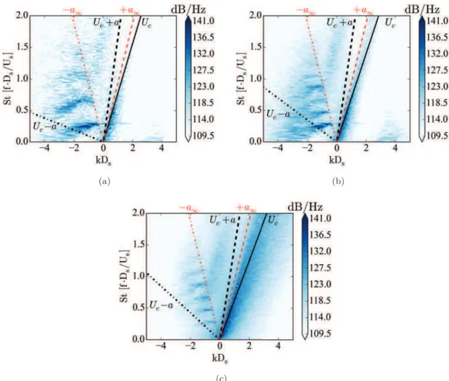
Figure 6.19 shows the transformed signal in the k − ω domain (see Eq. (3.6)). The results are averaged azimuthally to increase their accuracy. The acoustic lines are illustrated with a solid line and a dashed line for the positive and negative ambient sound speed ±a∞respectively. The

dotted line illustrates a convective velocity of 0.62Us. The region that lays within the acoustic lines represents the acoustic content of the signal. The region that lays outside corresponds to the hydrodynamic perturbations.

Some conclusions can be drawn from Fig. 6.19. Firstly, Fig. 6.19 (a) shows that the hydrody-namic lobe follows the convective velocity of the secondary jet, which exhibits an independence of the near-field with the primary flow. This could be expected, as the energy content of the secondary supersonic flow is much higher than that of the primary subsonic jet. The lobe cor-responding to the primary jet convective velocity may lay underneath the one of the secondary jet. This is an expected different behavior with respect to a subsonic dual stream jet [181] where both lobes are clearly present. Secondly, as expected, the hydrodynamic lobe is reduced when the probe is farther away from the axis as it is found at r/Ds = 1.7 in Fig. 6.19 (b). The shape of the k − ω distribution gives information about the dispersion of the pressure fluctuations. In a non-dispersive media the energy of the convective eddies would lay aligned perfectly with the convective velocity instead of presenting a lobe. The amount of disper-sion with respect to the convective line, gives an idea of how the perturbations can be seen as frozen [166]. Due to this dispersion, some hydrodynamics components would lie on the acoustic side of the k −ω distribution and vice-versa. The energy of the acoustic component is

(a) (b)

Figure 6.19: k − ω representation of the near-field flow at the probes located at (a) 0.85 Ds

and (b) 1.7 Ds from the axis. The solid and dashed lines represent the speed of sound. The

dotted line represents the convective velocity.

inside the jet. The acoustic content is clearly higher with respect to the subsonic jet of Tinney and Jordan [181] due to the fact that here, the acoustic captured is mostly due to the shock-cell noise that is being propagated upstream with a higher intensity whereas in their subsonic jet, it is generated by the mixing noise of fine-scale turbulence.

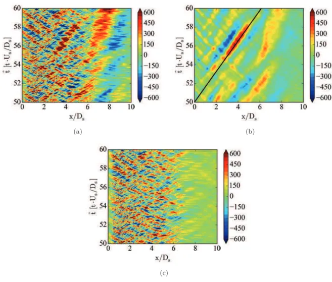
After the signal is transformed into the k − ω space, it can be reconstructed into the acoustic and the hydrodynamic component separately. Figures 6.20 (a), (b) and (c), display the original signal, the hydrodynamic signal and the acoustic signal respectively as a function of time and the axial position. The hydrodynamic signal, that is clearly appreciated in Fig. 6.20 (b), shows that it is well aligned with the convective speed Uc = 0.62Us noted by the solid black line as on the hydrodynamic lobe in Fig. 6.19 (b). As expected, some acoustic components traveling upstream are still present due to the dispersion of the signal at different frequencies. The acoustic component travels upstream and downstream at velocities greater than the sound speed a∞.

Once the flow is filtered in hydrodynamic and acoustic components, the spatial pressure cross-correlation can be studied for the original signal, and both filtered components. The spatial pressure cross-correlation gives not only information about the spatial size of the large tur-bulence structures, i.e. the wavelength of the wave-like pattern produced by the convected vortices but it also gives information about the characteristic acoustic wavelength being seen at each position of the array. This is done by computing the spatial cross-correlation on the hydrodynamic and the acoustic components separately. The spatial cross-correlation Rpp is computed using an analogous expression to Eq. (5.3) but using the pressure. Figure 6.21 de-picts the cross-correlation carried out at 3 different reference points along the axial direction averaged with all the azimuthal probes. The first point presented in Fig. 6.21 (a) is located at x/Ds = 0.85 and it shows that the acoustic correlation gives the same result as the original signal. At this axial position, the signal is mostly acoustics-originated at the shock-cells due to the fact that the shear-layer has not expanded enough in the radial direction. Farther

(a) (b)

(c)

Figure 6.20: Pressure on a single probe of an azimuthal array of 16 probes located at 0.85 Ds

from the axis which extends up to 10 Ds in the axial direction with an expansion angle of 8◦.

downstream of the jet, at x/Ds = 2.6 Fig. 6.21 (b) the acoustic correlation starts to deviate from the original signal. In particular, the negative side lobes around the maxima are closer together. At this location, the hydrodynamic perturbations are fully developed which can be seen from the larger negative lobes typical from a train of vortices. The last position displayed in Fig. 6.21 (c) is located at x/Ds = 4.2. At this position, the three correlations are fully different which emphasizes the importance of an acoustic-hydrodynamic separation of the flow when the measures are done close to the jet. Nonetheless, the three cross-correlations share a common crossing point which shows that the cross-correlation of the original signal keeps the main features of both the acoustics and the hydrodynamics of the flow.

−0.4 −0.2 0 0.2 0.4 0.6 0.8 1 0 0.5 1 1.5 2 Rpp x/D_s Full Hydrodynamic Acoustic (a) −0.4 −0.2 0 0.2 0.4 0.6 0.8 1 1 1.5 2 2.5 3 3.5 4 4.5 5 Rpp x/D_s Full Hydrodynamic Acoustic (b) −0.4 −0.2 0 0.2 0.4 0.6 0.8 1 2 3 4 5 6 7 Rpp x/D_s Full Hydrodynamic Acoustic (c)

Figure 6.21: Azimuthally averaged pressure cross-correlation of an azimuthal array of 16 probes

located at 0.85 Ds from the axis which extends up to 10 Ds in the axial direction with an

expansion angle of 8◦_{. Cross-correlations centered at (a) x/D}

s = 1, (b) x/Ds = 2 and (c)

x/Ds = 3.

The characteristic wavelength λ from Fig. 6.22 (a) can be computed by measuring the dis-tance between the negative peaks around the maxima of the correlations. As expected the characteristic wavelength of the acoustic component clearly differs from the one of the hydro-dynamic component. In addition, even though the cross-correlations shown in Fig. 6.21 are mostly different for the original signal and the two components, the characteristic wavelength of the original signal is similar to the one of the hydrodynamic component. The characteris-tic frequency can be computed from the characterischaracteris-tic wavelength by setting a characterischaracteris-tic

velocity as f = Uref/λ. The velocity chosen for the hydrodynamic component is the convec-tion velocity Uc = 0.62 Us. When dealing with the acoustic component, special care should be taken to the way the reference velocity is calculated. As it is illustrated by the sketch of Fig. 3.6, the characteristic pseudo-wavelength λ′ _{along the axis x}′ _{is the one that is being}

com-puted when measuring the distance between the negative peaks. Moreover, as it is expressed by Eq. (3.8) the velocity a′ _{on the same axis varies with the wavelength. The frequency is}

therefore computed as f = λ ′_a ∞ λ′1√_r2_{+ λ}′2_{− r}2 = a∞ ð r2_{+ λ}′2_{− r}, (6.4)

where λ′ _{on the numerator is simplified with the λ}′ _{used to compute the frequency f. Here,}

r being the perpendicular distance from noise source to the array, grows with x as the array has an expansion angle of 8 degrees. The resulting frequencies illustrated in Fig. 6.22 (b) give information about the peak frequencies of the convected vortices and the broadband shock-associated noise. The frequency of the hydrodynamic component starts at St = 0.65 but it decays up to a value of St = 0.17. On the other hand, the acoustic component shows good agreement with the frequency estimated by the mean shock-cell frequency f_{sh ≈ 1.82. The} reader needs to keep in mind that Eq. (6.4) is an approximation due to the fact that it only takes into account the Doppler effect of the shock-cell noise in the measured λ′ _{but not the}

fact that the noise comes from several noise sources distributed along the shock-cells.

!0 !0.5 !1 !1.5 !2 !2.5 !3 !3.5 !4 !0 !1 !2 !3 !4 !5 !6 !7 λ/D s x/D_s Full Hydrodynamic Acoustic (a) !0 !0.5 !1 !1.5 !2 !2.5 !3 !0 !1 !2 !3 !4 !5 !6 !7 Sts ![f!· !D s !/!U s ] x/D_s Hydrodynamic Acoustic (b)

Figure 6.22: (a) Characteristic wavelength computed with the spatial cross-correlation of an

azimuthal array of 16 probes located at 0.85 Dsand (b) the associated frequency with a reference

phase velocity.

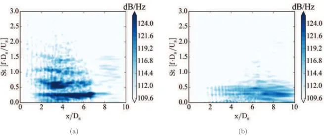
Figure 6.23 displays the SPL in dB/Hz computed for the original signal (a), the hydrodynamic component in (b) and the acoustic component in (c). The estimated frequencies computed with Eq. (3.8) and shown in 6.22 (b) are compared to the actual Sound Pressure Level (SPL) computed for each component. Good agreement is found for both the acoustic and the hydro-dynamic frequencies which confirms the validity of this approach. Here, the standard reference pressure of 2 · 10−5 _{Pa is used.}

(a) (b) (c)

Figure 6.23: Sound pressure level of an array of probes located at 0.85 Ds from the axis which

extends up to 10 Ds in the axial direction with an expansion angle of 8◦. (a) Full signal,

(b) hydrodynamic component and (c) supersonic component. The blue symbols represent the

characteristic frequencies of acoustic component computed with Eq. (3.8). The red symbols correspond to characteristic frequencies of the hydrodynamic component.

Sts = 2, x/Ds = 2 highlighted with the dashed circle. This ”banana-like” shaped signature that was already encountered for the supersonic under-expanded jet in Sec. 5.3.2 is character-istic of the Doppler effect of shock-cell noise. At the closest position to the axis, there are some higher frequency components that overlap with the shock-cell noise. This high frequency noise is generated at the region where the secondary shear-layer overcomes transition to turbulent regime.

6.3.3 Far-field acoustic field

In the previous section, the acoustics in the near-field were investigated. Here, the noise at the far-field at r/Ds = 30 from the inner nozzle exit plane is compared against the experimental measurements from VKI. The pressure perturbations from elsA were propagated to the far-field using the Ffowcs-Williams and Hawkings analogy presented in Sec. 3.3.1 and the SPL was averaged over 16 azimuthal probes in order to increase the smoothness of the spectra. On the other hand, the experimental measurements were obtained with a single array of microphones. The comparisons are shown in Fig. 6.25 for different angles computed from the jet direction. Overall, a good agreement is found in the positioning in frequency of the main peak of the broadband shock-associated noise at the angles where it is clearly present, that is, in the upstream angles in the range of 90◦_{− 120}◦_{. On the other hand, the amplitudes are off by 10}

dB. The far-field pressure spectra from the single jet matched well the numerical results and other experimental results as displayed in Fig. 5.15. Without fully discarding the possibility of an error in the measurements, some of the differences observed in the aerodynamics could

(a) (b) (c)

Figure 6.24: Acoustic component of the near-field in dB/Hz along different axial positions for

a line array with an angle of 7.3◦ _{at (a) r/D}

s= 0.85, (b) r/Ds= 1.3 and (c) r/Ds= 1.7. explain a difference in the far-field noise. An increase in the noise levels of the LES could be related to the higher rms values obtained in the secondary shear-layer as shown in Fig. 6.10. Also, the appearance of screech in experiments tends to lower by 1 to 2 dB the amplitude of the main peak of the BBSAN for supersonic under-expanded single jets [43]. Moreover, the fact that the first shock-cell presents a different pattern due to the axial shift of the experimental secondary nozzle (see Sec. 6.3.1) may change the stability of the jet and its associated noise. For comparison purposes, the spectra are shifted 10 dB in Fig. 6.26 (a). Due to the fact that the shock-cell lengths are smaller in the simulation, a shift is expected in the main peak of the BBSAN as it is inversely proportional to this parameter as stated by Eq. (5.2). The frequency axis is multiplied by a factor proportional to the mean variation of the shock-cell length shown in Table 6.3 as fmod= Lexp._sh Lnum. sh forig, (6.5)

where forig is the original frequency vector, Lexp._sh is the average experimental shock-cell length and Lnum.

sh is the average numerical shock-cell length. The modified frequency vector is then used for the experimental results as it is shown in Fig. 6.26 (b). The peak of the BBSAN agrees well with the experimental spectra when the new modified frequency vector is defined.

6.3.4 Power spectral density axial distribution

The data extracted in the axis (AXIS) can be analyzed in terms of power spectral density in the axial range 0 < x/Ds< 10. When the pressure energy distribution is transformed into the frequency-wavenumber domain (Fig. 6.27 (a)), different tones are found in the negative part

!90 !95 !100 !105 !110 !115 !120 !0.01 !0.1 !1 !10 SPL![dB/St] St![f!·!D_s!/!U_s] num.!elsA exp.!VKI! θ!=!30!deg !90 !95 !100 !105 !110 !115 !120 !0.01 !0.1 !1 !10 SPL![dB/St] St![f!·!D_s!/!U_s] num.!elsA exp.!VKI! θ!=!40!deg !90 !95 !100 !105 !110 !115 !120 !0.01 !0.1 !1 !10 SPL![dB/St] St![f!·!D_s!/!U_s] num.!elsA exp.!VKI! θ!=!50!deg !90 !95 !100 !105 !110 !115 !120 !0.01 !0.1 !1 !10 SPL![dB/St] St![f!·!D_s!/!U_s] num.!elsA exp.!VKI! θ!=!60!deg !90 !95 !100 !105 !110 !115 !120 !0.01 !0.1 !1 !10 SPL![dB/St] St![f!·!D_s!/!U_s] num.!elsA exp.!VKI! θ!=!70!deg !90 !95 !100 !105 !110 !115 !120 !0.01 !0.1 !1 !10 SPL![dB/St] St![f!·!D_s!/!U_s] num.!elsA exp.!VKI! θ!=!80!deg !90 !95 !100 !105 !110 !115 !120 !0.01 !0.1 !1 !10 SPL![dB/St] St![f!·!D_s!/!U_s] num.!elsA exp.!VKI! θ!=!90!deg !90 !95 !100 !105 !110 !115 !120 !0.01 !0.1 !1 !10 SPL![dB/St] St![f!·!D_s!/!U_s] num.!elsA exp.!VKI! θ!=!100!deg !90 !95 !100 !105 !110 !115 !120 !0.01 !0.1 !1 !10 SPL![dB/St] St![f!·!D_s!/!U_s] num.!elsA exp.!VKI! θ!=!110!deg !90 !95 !100 !105 !110 !115 !120 !0.01 !0.1 !1 !10 SPL![dB/St] St![f!·!D_s!/!U_s] num.!elsA exp.!VKI! θ!=!120!deg

Figure 6.25: Far-field sound pressure level at r/Ds = 30 from the primary nozzle exit for

!90 !95 !100 !105 !110 !115 !120 !0.01 !0.1 !1 !10 SPL![dB/St] St![f!·!D_s!/!U_s] num.!elsA exp.!VKI! θ!=!120!deg (a) !90 !95 !100 !105 !110 !115 !120 !0.01 !0.1 !1 !10 SPL![dB/St] St![f!·!D_s!/!U_s] num.!elsA exp.!VKI! θ!=!120!deg (b)

Figure 6.26: Far-field acoustics at r/Ds= 30 from the primary nozzle exit at 120◦ with (a) a

shift of 10 dB applied and (b) a shift in frequency is also applied.

decomposition is carried out for the data sets at the primary (LIP P) and secondary (LIP S) lip-lines shown in Fig. 6.27 (b) and Fig. 6.27 (c) respectively. As it can be seen in Fig. 6.27, the patterns are mainly contained between the line that represents the acoustic ambient velocity a∞ and the mean negative acoustic velocity of the corresponding data set. The convective

velocity as well as the local sound speed change with the axial position. For all data sets displayed in Fig. 6.27, the convective velocity Uc = 0.62Us lays on the lobe of the downstream convective velocity.

Theoretically, in a dual stream jet whose primary jet is subsonic, four sets of negative traveling waves could be detected in the flow. First, a wave that is generated by the shock-cell noise of the secondary shear-layer could enter the supersonic secondary stream in the same way as it happens for a supersonic single jet (see Fig. 5.28). Moreover, these waves would travel up to the shear-layer of the primary inner subsonic stream which then would be convected as a regular wave inside. This wave could be again convected outside if it has not been dissipated already. Second, the shock-cell noise generated in the primary inner shear-layer could be directly convected upstream throughout the inner subsonic jet. Third, a set of trapped acoustic waves generated at the end of the inner potential core could be formed and travel through the subsonic jet as it was demonstrated by Towne et al. [211] for subsonic single jets at Mach numbers about M = 0.9. At certain frequencies, these trapped waves resonate due to the end conditions provided by the nozzle and the streamwise contraction of the potential core. Last, upstream traveling parasitic waves generated at the exit boundary of the domain could also appear but are not contemplated in this study as the simulation was carried out with non-reflective boundary conditions and a sponge layer that would attenuate them.

The positive and negative traveling waves can be analyzed independently by reverting the transformation of the data sets from the frequency-wavenumber domain to the time-space domain by only using the positive or the negative wavenumbers. Figure 6.28 shows the positive and negative pressure waves for the AXIS and Fig. 6.29 for the data sets LIP P and LIP S which are averaged among the 16 azimuthally distributed probes at each axial location. The negative traveling waves are now clearly visible, especially for the data sets in both shear-layers that are superimposed with the downstream traveling vortices. A problem that arises with this separation is the fact that the axial discretization of the probes changes after x/Ds= 7 from 0.1 D to 1 D . Even though the probes were interpolated into a uniform mesh size before

(a) (b)

(c)

Figure 6.27: Frequency-wavenumber energy distribution of the pressure for the data set (a) AXIS, (b) LIP P and (c) LIP S

investigated in this work. The different main distinguishable tones for all three pressure data sets are summarized in Table 6.5.

Data Set St1 St2 St3 St4 St5 St6

AXIS 0.27 0.53 0.64 1.07 1.39 LIP P 0.27 0.46 0.64 0.86 1.03 1.22

LIP S 0.27 0.46 0.64 0.86 1.03 1.22

Table 6.5: Frequency tones observed for the pressure energy distribution at the AXIS, LIP P and LIP S data sets. The Stouhal number is defined based on the secondary diameter and the secondary perfectly expanded jet exit velocity.

In order to understand better the excited frequencies and its axial localization, four different axial positions have to be evoked. First, the shock-cells are mainly located between 0 <

x/Ds < 4, second, the mean flow of the secondary stream, even if it does not clearly show a

shock-cell pattern, it is still supersonic up to x/D ≈ 5.75, which could be taken as the end of the secondary potential core. Third, the secondary stream merges with the primary between 6.25 < x/D < 8. And last, the end of the primary potential core could be considered to be about x/D ≈ 9, which is elongated due to the merging with the secondary stream.

The PSD on AXIS presented in Fig. 6.28 demonstrates that the identified tones belong indeed to the negative traveling waves reaching up to Sts= 2 (Fig. 6.28 (a)). The first tone St1 has

an extreme at the position where both concentric jets fully merge (about x/Ds= 8) and it is being excited up to an upstream distance of x/Ds= 2. The remaining tones exhibit a higher intensity in the range 2 < x/Ds < 6. On the other hand, the positive traveling waves shown in Fig. 6.28 (b) are accumulated below St = 0.5 which are characteristic lower frequencies for the hydrodynamic perturbations that are convected downstream. The energy distribution for the original axial velocity displayed in Fig. 6.28 (b) presents a peak at St = 0.5 and x/Ds= 6, farther downstream, the energy distribution levels grow due to the mixing of the jet after the end of the potential cores.

A similar energy content of the pressure energy distribution is found for the LIP P and LIP S data sets shown in Fig. 6.29. At this last location it is clear that the separation in negative and positive traveling waves is limited and a discontinuity is distinguishable where the discretization changes. Some of the peaks appear to be harmonics of a fundamental frequency. The peaks are not clearly defined in the frequency domain which suggests that the group velocity is not singular but broadband. The impact of the shock-cells is seen in the pressure energy distribution with a higher level in the compression zone. The results found at LIP P and LIP S present two sets of patterns. The first one at the lower frequencies is situated between the end of the shock-cell region and the start of the merging region around 4 < x/Ds< 7, which shares a portion of the supersonic (non-shocked) region of the secondary stream. The higher frequencies clearly are in the region of the shock-cells between 2 < x/Ds < 4. Additionally, LIP P (Fig. 6.29 (c)) presents a similar distribution for the positive traveling waves than in AXIS. The positive traveling waves at LIP S shown in Fig. 6.29 (d) exhibit a logarithmic shape, with higher frequencies excited close to the nozzle lip, and lower frequencies excited when the shear-layer is developed.

(a) (b)

Figure 6.28: Frequency-space energy distribution along the axial direction for the data set AXIS of (a) the negative traveling pressure waves and (b) the positive traveling pressure waves. Towne et al. [211] which has a high receptivity to establish trapped acoustic waves, however, here the case of consideration is the one of a dual-stream with a supersonic under-expanded secondary stream. Moreover, the PSD shows a great resemblance with the patterns obtained for the supersonic under-expanded single jet. The patterns present at the AXIS extend up to the merging point of both streams for the lower frequencies, and then they reduce their axial extension for higher frequencies. On the other hand, the PSD computed at LIP P and LIP S are composed of two sets of patterns. The first one for the lower frequencies is situated between the end of the shock-cell region and the start of the merging region, which shares a portion of the supersonic (non-shocked) region of the secondary stream.

The data sets located in the primary and secondary lip-lines are composed of 16 azimuthal probes and they can be further decomposed into the azimuthal modes as explained in Sec. 3.3.3. Here, only the decomposition of the negative traveling waves is investigated as they are the only ones that present a noticeable pattern. Only the first 3 modes and the mean value are used as they are the ones with the highest energy content and they are the less polluted by the aliasing as discussed in Appx. B. The results are shown in Fig. 6.30 and 6.31 for the LIP P and LIP S respectively and the associated frequencies presented in Table 6.5 at each mode are summarized in Table 6.6.

mode 0 mode 1 mode 2 mode 3

LIP P and LIP S St1, St3 St2, St4 St3, St5 St4, St6

Table 6.6: Frequency tones observed for the pressure energy distribution at the LIP P and LIP S data sets according to the azimuthal mode.

As it can be seen from Table 6.6, the different azimuthal modes share some of the frequencies. This could imply that the generation of the modes are linked and corresponds to the same phenomena encountered for the single jet, the shock-cell noise. Moreover, two main regions where the patterns are found share common azimuthal modes.

(a) (b)

(c) (d)

Figure 6.29: Frequency-space energy distribution along the axial direction for the data set LIP P on the left column and LIP S on the right column of (a),(b) the negative traveling pressure waves and (c),(d) the positive traveling pressure waves.

(a) (b)

(c) (d)

Figure 6.30: Frequency-space energy distribution along the axial direction for the data set LIP P of the negative pressure traveling waves for the azimuthal modes: (a) mode 0, (b) mode 1, (c) mode 2 and, (d) mode 3.

(a) (b)

(c) (d)

Figure 6.31: Frequency-space energy distribution along the axial direction for the data set LIP S of the negative pressure traveling waves for the azimuthal modes: (a) mode 0, (b) mode 2 and, (b) mode 3.

6.3.5 Wavelet analysis

The wavelet-based methodology described in Ch. 4 implemented to identify and extract the characteristic events of the single jet (Sec. 5.3.6) is applied in this section to the data sets AXIS, LIP P, LIP S and NF1D. The wavelet parameters set for the single jet are kept constant for this case of study. Moreover, a similar representation of the results is discussed (see Sec. 5.3.6). The two-dimensional cross-conditioning is performed by the average of only the positive y/Ds> 0 and negative y/Ds< 0 regions of the cut at z/Ds= 0. Moreover, the azimuthal decomposition is used as well in order to identify the shape of the events of each mode with a two-dimensional cross-conditioning averaged over an axial cut. The equivalent frequencies and axial positions of the reference point used to detect the events are presented in the following for each variable and data set.

Axis probes analysis

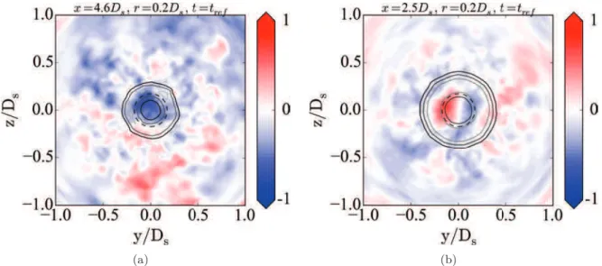
The cross-conditioning applied to the AXIS is displayed in Fig. 6.32. The axial velocity events were computed at an equivalent frequency of Sts(s) = 0.5, that is the frequency where the energy distribution at the axial position x/Ds = 5 exhibits a higher energy distribution. The auto-conditioning of the axial velocity (i.e. the plot of the axial velocity using as a reference the events obtained with the same variable) is shown in Fig. 6.32 (a). Down traveling waves that grow with the axial direction are originated achieving a local maximum about x/Ds= 5, that is the position where the urms is maximum. The cross-conditioning with the pressure displayed in Fig. 6.32 (b) presents two different waves. The first wave is found in the range 2 < x/Ds < 4 where the shock-cells are concentrated and it is demonstrated later that they are waves traveling upstream. The impact of the shock-cells on the amplitude of the signature is clearly illustrated by all the peaks in this region. The second wave, traveling downstream is the corresponding signature of the velocity displayed in Fig. 6.32 (a), phased π rad (negative amplitude). The two-dimensional auto-conditioning shown in Fig. 6.33 (a) presents events that are extended in the radial direction up to 0.5 Ds and shifted with the higher velocity of the secondary stream. The two-dimensional cross-conditioning depicted in Fig. 6.33 (b) shows that the impact on the pressure is extended radially more than 1 Ds. In the detailed region, the negative traveling waves are present in the subsonic primary jet only.

Next, the cross-conditioning using the negative traveling pressure waves on the AXIS is dis-cussed using as reference frequency Sts(s) = 0.64. This equivalent frequency is used as it is one of the frequencies that presents a higher number of events at x/Ds = 3. Figure 6.32 (c) shows the cross-conditioning between pneg and the axial velocity u. A wave with constant am-plitude traveling downstream is captured at a downstream position, where the event is located. This could mean that the downstream traveling waves are coupled to the events detected at x/Ds = 3. The amplitude of the down-traveling waves grows in the region of the shock-cells and then it keeps a constant mean value. Figure 6.34 (a) exhibits a similar pattern as the one obtained with the axial velocity events shown in Fig. 6.33 (a). The auto-conditioning of the negative traveling pressure waves is displayed in Fig. 6.32 (d). Taking a look at the envelope of the signature, it seems that different events are captured as well. The positive envelope grows with the shock-cells and then it is constant up to x/Ds = 6, where it decays. On the other hand, the negative envelope presents two minima at x/Ds = 3 and x/Ds = 6. As it is discussed later, the second peak could correspond to an azimuthal mode 0, while the first peak

−40 −30 −20 −10 0 10 20 30 40 0 2 4 6 8 10 u’ [m/s] x/D_s (a) −3000 −2000 −1000 0 1000 2000 3000 0 2 4 6 8 10 p’ [Pa] x/D_s (b) −40 −30 −20 −10 0 10 20 30 40 0 2 4 6 8 10 u’ [m/s] x/D_s (c) −4000 −3000 −2000 −1000 0 1000 2000 3000 4000 0 2 4 6 8 10 p’ [Pa] x/D_s (d) −40 −30 −20 −10 0 10 20 30 40 0 2 4 6 8 10 u’ [m/s] x/D_s (e) −4000 −3000 −2000 −1000 0 1000 2000 3000 4000 0 2 4 6 8 10 p’ [Pa] x/D_s (f)

Figure 6.32: Cross-conditioning of (a) u−u, (b) u−p, (c) pneg−u, (d) pneg−p, (e) ppos−u

and (f) ppos− p from AXIS where the first variable is the one used to locate the events and the

second variable is the one plotted. The dash black line represents the envelope of the signature for all axial positions. The vertical dashed line represents the axial position where the events are located.