Random walks and diffusion on networks

(1)

RESEARCH OUTPUTS / RÉSULTATS DE RECHERCHE

Author(s) - Auteur(s) :

Publication date - Date de publication :

Permanent link - Permalien :

Rights / License - Licence de droit d’auteur :

Bibliothèque Universitaire Moretus Plantin

Institutional Repository - Research Portal

Dépôt Institutionnel - Portail de la Recherche

researchportal.unamur.be

University of Namur

Random walks and diffusion on networks

Masuda, Naoki; Porter, Mason A.; Lambiotte, Renaud

Published in:

Physics Reports

DOI:

10.1016/j.physrep.2017.07.007

Publication date:

2017

Document Version

Publisher's PDF, also known as Version of record

Link to publication

Citation for pulished version (HARVARD):

Masuda, N, Porter, MA & Lambiotte, R 2017, 'Random walks and diffusion on networks', Physics Reports, vol.

716-717, pp. 1-58. https://doi.org/10.1016/j.physrep.2017.07.007

General rights

Copyright and moral rights for the publications made accessible in the public portal are retained by the authors and/or other copyright owners and it is a condition of accessing publications that users recognise and abide by the legal requirements associated with these rights. • Users may download and print one copy of any publication from the public portal for the purpose of private study or research. • You may not further distribute the material or use it for any profit-making activity or commercial gain

• You may freely distribute the URL identifying the publication in the public portal ? Take down policy

If you believe that this document breaches copyright please contact us providing details, and we will remove access to the work immediately and investigate your claim.

(2)

Contents lists available atScienceDirect

Physics Reports

journal homepage:www.elsevier.com/locate/physrep

Random walks and diffusion on networks

Naoki Masuda

a,

*

, Mason A. Porter

b,c,d

, Renaud Lambiotte

c

a_{Department of Engineering Mathematics, University of Bristol, Bristol, UK} b_{Department of Mathematics, University of California Los Angeles, Los Angeles, USA} c_{Mathematical Institute, University of Oxford, Oxford, UK}

d_{CABDyN Complexity Centre, University of Oxford, Oxford, UK}

a r t i c l e i n f o

Article history:

Accepted 25 July 2017 Available online 31 August 2017 Editor: I. Procaccia Keywords: Random walk Network Diffusion Markov chain Point process a b s t r a c t

Random walks are ubiquitous in the sciences, and they are interesting from both theoretical and practical perspectives. They are one of the most fundamental types of stochastic processes; can be used to model numerous phenomena, including diffusion, interactions, and opinions among humans and animals; and can be used to extract information about important entities or dense groups of entities in a network. Random walks have been studied for many decades on both regular lattices and (especially in the last couple of decades) on networks with a variety of structures. In the present article, we survey the theory and applications of random walks on networks, restricting ourselves to simple cases of single and non-adaptive random walkers. We distinguish three main types of random walks: discrete-time random walks, node-centric continuous-time random walks, and edge-centric continuous-time random walks. We first briefly survey random walks on a line, and then we consider random walks on various types of networks. We extensively discuss applications of random walks, including ranking of nodes (e.g., PageRank), commu-nity detection, respondent-driven sampling, and opinion models such as voter models.

Contents

1. Introduction... 2

2. Random walks on the line... 4

2.1. Discrete time... 4

2.2. Continuous time... 5

3. Random walks on networks... 6

3.1. Notation... 6

3.2. Discrete time... 7

3.2.1. Definition and temporal evolution... 7

3.2.2. Stationary density... 7

3.2.3. Relaxation time... 9

3.2.4. Exit probability... 11

3.2.5. Mean first-passage and recurrence times... 11

3.2.6. Cover time... 16

3.3. Continuous-time random walks (CTRWs)... 17

3.3.1. Node-centric versus edge-centric random walks... 17

3.3.2. Active versus passive random walks... 19

4. Random walks on generalized networks... 23

*

Corresponding author.

E-mail address:[email protected](N. Masuda). http://dx.doi.org/10.1016/j.physrep.2017.07.007

(3)

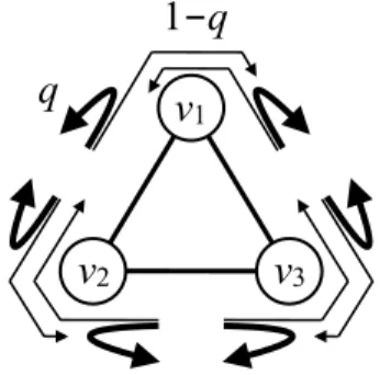
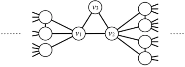
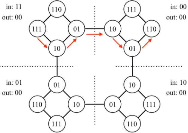
4.1. Multilayer networks... 23 4.2. Temporal networks... 24 4.2.1. Activity-driven model... 25 4.2.2. Memory networks... 26 5. Applications... 30 5.1. Search on networks... 30 5.2. Ranking... 30 5.2.1. PageRank... 31 5.2.2. Laplacian centrality... 32 5.2.3. TempoRank... 32

5.2.4. Random-walk betweenness centrality... 33

5.2.5. Discrete-choice models... 36

5.3. Community detection... 37

5.3.1. Markov-stability formulation of modularity... 38

5.3.2. Walktrap... 39

5.3.3. InfoMap... 39

5.3.4. Local community detection... 41

5.3.5. Multilayer modularity... 41

5.4. Core–periphery structure... 42

5.5. Diffusion maps... 43

5.6. Respondent-driven sampling... 44

5.7. Consensus probability and time of voter models... 45

5.8. DeGroot model... 47

6. Conclusions and outlook... 49

Acknowledgments... 50

References... 50

1. Introduction

Random walks (RWs) are popular models of stochastic processes with a very rich history [1–5].1 The term ‘‘random walk’’ was coined by Karl Pearson [6], and the study of RWs dates back to the ‘‘Gambler’s Ruin’’ problem analyzed by Pascal, Fermat, Huygens, Bernoulli, and others [7]. Additionally, Albert Einstein formulated stochastic motion (in the form of ‘‘Brownian motion’’) of particles in continuous time due to their collisions with atoms and molecules [8]. Theoretical developments have involved mathematics (especially probability theory), computer science, statistical physics, operations research, and more. RW models have also been applied in various domains, ranging from locomotion and foraging of animals [9–12], the dynamics of neuronal firing [13,14] and decision-making in the brain [15,16] to population genetics [17], polymer chains [18,19], descriptions of financial markets [20,21], evolution of research interests (through RWs on problem space) [22], ranking systems [23], dimension reduction and feature extraction from high-dimensional data (e.g., in the form of ‘‘diffusion maps’’) [24,25], and even sports statistics [26,27]. RW theory can also help predict arrival times of diseases spreading on networks [28]. There exist several monographs and review papers on RWs. Many of them treat RWs on classical network topologies, such as regular lattices (e.g., Zd_{) and Cayley trees (i.e., trees in which each node has the same number} of neighboring nodes, which we henceforth call the node ‘‘degree’’) [4,29–35]. Other monographs and surveys focus on RWs on fractal structures, revealing diffusion properties that are ‘‘anomalous’’ compared to RWs on regular lattices or Euclidean spaces (i.e., Rd_{) [}₃₂_,₃₆_–₄₀_{]. Other literature treats RWs on finite networks, which are equivalent to a finite Markov chain (in} the discrete-time case) [1,32,41,42] and are at the core of several stochastic algorithms.

In parallel, ‘‘network science’’ has emerged in recent years as a central approach to the study of complex systems [43–46]. Networks are a natural representation of systems composed of interacting elements and allow one to examine the impact of structure on the dynamics and function of a system (as well as the impact of dynamics and function on network structure). Examples include friendship networks, international relationships, gene-regulatory networks, food webs, airport networks, the internet, and myriad more. In each case, one can represent the system’s connectivity structure as a set of nodes (representing the entities in the system) and edges (representing interactions among those entities). The study of networks is highly interdisciplinary, and it integrates theoretical and computational tools from subjects such as applied mathematics, statistical physics, computer science, engineering, sociology, economics, biology, and other domains. Many networks exhibit complex yet regular patterns that are explainable (sometimes arguably) by simple mechanisms. Network science has also had a strong impact on the understanding of dynamical processes because of the critical role of structure on spreading processes, synchronization, and others [47–49]. As with RWs, numerous books and review papers have been written on networks, including textbooks [44,45,50–52], general review articles [46,53], and more specialized reviews on topics such

1_See_{https://www.youtube.com/watch?v=stgYW6M5o4k}_{for an introduction to random walks for a public audience from the U.S. Public Broadcasting}

(4)

as dynamical processes on networks [48,49,54], connections to statistical physics [55,56], temporal networks [57–59], multilayer networks [60–62], and community structure [63–65].

The main purpose of the present review is to bring together two broad subjects – RWs and networks – by discussing their many interconnections and their ensuing applications. RWs are often used as a model for diffusion, and there has been intense research on the impact of network architecture on the dynamics of RWs. Moreover, nontrivial network structure paves the way for different definitions of RWs, and different definitions can be ‘‘natural’’ from some perspective, while leading to different diffusive processes on the same network. Finally, RWs are at the core of several algorithms to uncover structural properties in networks. We will discuss these points further in the next three paragraphs.

First, RWs are often used as a model for diffusion, and there has been intense research on the impact of network architecture on the dynamics of RWs. The finiteness of a network – along with properties such as degree heterogeneity, community structure, and others – can make diffusion on networks both quantitatively and even qualitatively different from diffusion on regular or infinite lattices. RWs on networks are an example of a Markov chain in which the set of nodes is the state space and the transition probabilities depend on the existence and weights of the edges between nodes. In this review, we will include a summary of results on the dependence of dynamical properties – including stationary distribution and mean first-passage time – on structural properties of an underlying network.

Second, the irregularity of underlying network structure opens the door for different definitions of RWs. Each is ‘‘natural’’ from some perspective, but they lead to different diffusive processes even when considering the same network. For example, it is useful to distinguish between discrete-time and continuous-time RWs. On networks in which degree (i.e., the number of neighbors) is heterogeneous (i.e., it depends on the node), one needs to subdivide continuous-time RWs further into two major types, depending on whether the random events that induce walker movement are generated on nodes or edges and corresponding to different types of propagators (normalized versus unnormalized Laplacian matrices). Different literatures use different variants of RWs, often implicitly. We distinguish different types of RWs and clarify the relationship between them, and we discuss formulations and results that are informed by empirical networks (such as networks with heavy-tailed degree distributions, multilayer networks, and temporal networks).

Finally, RWs lie at the core of many algorithms to uncover various types of structural properties of networks. Consider the notion of identifying ‘‘central’’ nodes, edges, or other substructures in networks [44]. A powerful set of diagnostics (e.g., PageRank [23,66] and eigenvector centrality [67]) are derived based on recursive arguments of the type ‘‘a node is important if it is connected to many important nodes’’, and such derivations often rely on the trajectories of random walkers. Similarly, flow-based algorithms, based on trajectories of dynamical processes (e.g., RWs) being trapped within certain sets of node for a long time, are helpful for discovering mesoscale patterns in networks [65,68]. These techniques and algorithms open a wealth of applications that go well beyond classical applications of RWs. Their design benefits both explicitly and implicitly from developing an understanding of how RW dynamics are influenced by network structure and how different types of RWs behave on the same network.

There has been a vast amount of research on RWs on networks, and it is scattered across disparate corners of the scientific literature. It is impossible to cover everything, and we choose specific subsets of it to make our review cohesive, although we will occasionally include pointers to other parts of the landscape. First, we focus on the most standard types of RWs, in which a random walker moves to a neighbor with a probability proportional to edge weight, and their very close relatives. We only very rarely mention some of the numerous other types of RWs, which include correlated RWs [69], self-avoiding RWs [4,70,71], zero-range processes [72], multiplicative random processes [73,74], adaptive RWs (including reinforced RWs [75]), branching RWs [76], Lévy flights [34,35], elephant RWs [77], quantum walks [78,79], intermittent RWs [80], persistent RWs [81], starving RWs [82–84], mortal RWs [85], and so on. These processes are of course fascinating, and many of the different flavors of RWs are often developed with specific motivation from an application (e.g., a Pac-Man-like ‘‘hungry RW’’ [86] has been used as a model for chemotaxis in a porous medium), are often inspired by applications, such as animal movement [10,12] or financial markets [21], and one can find discussions of different flavors of RWs in Refs. [4,34,35]. Second, we will not cover many results for RWs on particular generative models of networks, except that we do give extensive attention to first-passage times for fractal and pseudo-fractal network models (see Section3.2.5). Third, we will not discuss various important, rigorous results from mathematics and theoretical computer science. For such results, see [1,4,30,41,42]. We focus instead on results that we believe give physical insight on RW processes and their applications.

As a final warning, we focus almost exclusively on diffusive processes in which the total number of walkers (or, equivalently, the total probability of observing a walker) is a conserved quantity.2 _{The only exceptions are in Section} 5.3.4, where a type of RW in which the number of walkers decreases in time is used in a community-detection algorithm called Nibble, and in Section5.7, where we use ‘‘coalescing RWs’’ as an analytical tool. As we will see, this conservation rule translates into certain properties of the operator that drives the RW process. When transposed, the operator leads naturally to linear models for consensus dynamics (see Sections5.7and5.8). Among notable non-conservative processes, which we do not cover in this review, are classical epidemic processes [48,49,89,90], in which the number of entities (e.g., viruses or infected individuals) varies over time. In the linear regime, corresponding to a small number of infected nodes, the propagator of infection events in simple epidemic processes such as susceptible–infected (SI) and susceptible–infected–recovered (SIR) models are the adjacency matrix [91,92]. In contrast, a propagator of an RW is a type of Laplacian matrix, as we will discuss in detail in Section3. If all nodes have the same degree, these Laplacian and adjacency matrices are related linearly, and their

(5)

dynamics are essentially the same [59,93]. However, they are generically different for heterogeneous networks, such as when degree depends on node identity. Therefore, the difference between conservative dynamics (described by a Laplacian matrix) and non-conservative dynamics (described by the adjacency matrix) tends to be more striking for heterogeneous than for homogeneous networks. Other spreading models that are also beyond the scope of this work include threshold models of social contagions [49,94] (e.g., for modeling adoption of behaviors) and reaction–diffusion dynamics [95].

The rest of our review proceeds as follows. In Section2, we discuss RWs on the line. In Section3, we give a lengthy presentation of RWs on networks. We then discuss RWs on multilayer networks in Section4.1 and RWs on temporal networks in Section4.2. We discuss applications in Section5, and we conclude in Section6.

2. Random walks on the line

In this section, we review some basic properties of RW processes on one-dimensional space (i.e., the infinite line). This section serves as a primer to later sections, in which we examine RWs on general networks. In this and later sections, we carefully distinguish between discrete-time and continuous-time models.

2.1. Discrete time

Consider a discrete-time RW (DTRW) process on the infinite line, which we identify with R1

_≡

R. There is a single walker. At each discrete time step, it moves from some point to some other point, including the case of moving from a point to itself. The length and direction of the move are both random variables. We assume that the probability that a walker located at x moves to the interval

[

x

+

r

,

x

+

r

+

∆r

]

in one step is equal to f (r)∆r. The normalization is

∫

∞

−∞f (r)dr

=

1, and we assume

that moves at different times are independent.

We derive the probability density p(x

;

n) that a random walker is located at a point x

∈

_{R after n steps. (For emphasis, we}

sometimes use the term ‘‘discrete time’’ or ‘‘event time’’ for n.) The master equation is given by

p(x

;

n)

=

∫

∞

−∞

f (x

−

x′)p(x′

;

n

−

1)dx′

.

(1) It is convenient to solve Eq.(1)for general x and n in the Fourier domain. We define the Fourier transform by

ˆ

p(k

;

n)

≡

∫

∞

−∞

p(x

;

n)e−ikxdx (2)

and the inverse Fourier transform by

p(x

;

n)

≡

1 2

π

∫

∞ −∞

ˆ

p(k

;

n)eikx_dk

_.

₍₃₎

Note thatp(

ˆ

−

k

;

n) is the ‘‘characteristic function’’ of a random variable x with probability density p(x

;

n). The Fourier

transformf (k) of f (x) is sometimes called the ‘‘structure function’’ of the RW. The Taylor expansion of

ˆ

p(k

ˆ

;

n) around k

=

0 yields

ˆ

p(k

;

n)

=⟨

e−ikx

⟩

=

1

−

ik

⟨

x

⟩ −

1 2k 2

_⟨

_x2

_{⟩ +}

_O(k3₎

_,

₍₄₎

where

⟨·⟩

is the expectation unless we state otherwise. One can thereby obtain moments of p(x

;

n) from the derivatives of

ˆ

p(k

;

n) at k

=

0.

The Fourier transform maps a convolution, such as Eq.(1), to a product; and Eq.(1)thus yields

ˆ

p(k

;

n)

= ˆ

f (k)p(k

ˆ

;

n

−

1)

.

(5) If a random walker is located initially at x

=

0, we obtain p(x

;

0)

=

δ

(x), where

δ

(x) is the Dirac delta function, which has Fourier transformp(k

ˆ

;

0)

=

1. We thereby obtain

ˆ

p(k

;

n)

=

[

ˆ

f (k)

]

n

.

(6)

Using the inverse Fourier transform in Eq.(3), we obtain a formal solution for p(x

;

n) in the time domain: p(x

;

n)

=

1 2

π

∫

∞ −∞

[

ˆ

f (k)

]

n eikxdk

.

(7)

The qualitative behavior of the solution in Eq.(7)depends on the details of the structure functionf (k). However, the

ˆ

asymptotic behavior of the RW as n

→ ∞

depends only on some of the properties off (k). When the first two moments of

ˆ

f (k) are finite, the solution converges to the Gaussian profile p(x

;

n)

=

1

(2

π

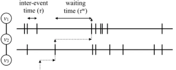
Dn)1/2e −(x−vn)2

(6)

Fig. 1. Schematic of the standard continuous-time random walk (CTRW) on a one-dimensional lattice. (a) The position x of the walker in physical time t is

described by p(x;t). Note that tnrepresents the time of the nth move. (b) The position of the walker after n moves is described by p(x;n).

where

v ≡ ⟨

r

⟩

and D

≡ ⟨

(r

−⟨

r

⟩

)2

⟩

/

2. Eq.(8)implies that the variance of x grows linearly with time. This result is the ‘‘central limit theorem’’ for the sum of the sizes of the moves, which are independent random variables. This asymptotic regime is well-defined because the underlying space (i.e., the line) is infinitely large. One can derive these results in a similar manner when the underlying space is discrete (e.g., a one-dimensional lattice) [2,4,30,31]. In situations in which the second moment of the structure function diverges, the process exhibits superdiffusion and the probability profile converges to so-called ‘‘Lévy distributions’’ [34,35].

2.2. Continuous time

In this section, we consider continuous-time RWs (CTRWs), which incorporate the timing of moves [4,5,30,34,35,96]. We assume that a walker waits between two moves for a duration

τ

that independently obeys the probability density function

ψ

(

τ

). In other words, the move events are generated by a renewal process [3]. If

τ =

1 with probability 1, the CTRW reduces to the DTRW described in Section2.1. In a standard CTRW, one assumes that the time of a move event and the selection of a destination in a given move are independent. Therefore, a combination of

ψ

(

τ

) and f (r), where r is the displacement in a single move, completely determines the dynamical properties of a random walker.

Let tndenote the time of the nth move. By definition, tn

=

∑

n

i=1

τ

i, where each

τ

iis independent and identically distributed (i.i.d.) and drawn from some distribution

ψ

(

τ

). Additionally, we can write

p(x

;

t)

=

∞

∑

n=0

p(x

;

n)p(n

,

t)

,

(9)

where p(x

;

t) is the probability that the walker is located at x at time t, the quantity p(x

;

n) is the probability that the walker

is located at x after n steps, and p(n

,

t) is the probability density that the walker has moved n times at time t. Note that it

is crucial to distinguish p(x

;

t) and p(x

;

n), and we illustrate the difference between these probabilities with a schematic in

Fig. 1. Eq.(9)reflects the fact that a walker can visit x at time t after some number n of steps.

The probability p(x

;

n) is given by the same solution, Eq.(7), as for the DTRW. To obtain p(x

;

t) from Eq.(9), we need to examine p(n

,

t), and we thus need to consider a renewal process generated by

ψ

(

τ

). According to the elementary renewal theorem [97], the mean of n at time t is

⟨

n

⟩ =

t

⟨

τ⟩

.

(10)

Eq.(10)indicates that n(t) grows linearly with time on average, irrespective of the details of the distribution

ψ

(

τ

). However, realized values of n are random, inducing heterogeneity in the length of the RW ‘‘trajectory’’ (i.e., the walk measured in terms of the number of moves) observed at a given time t.

When the CTRW is driven by a Poisson process,

ψ

(

τ

) is the exponential distribution (i.e.,

ψ

(

τ

)

=

β

e−βτ

). In this case, n obeys the Poisson distribution with mean

β

t. That is,

p(n

,

t)

=

(

β

t)

n

!

e

−βt

_.

₍₁₁₎

It requires some effort to derive p(n

,

t) when

ψ

(

τ

) is a general distribution. To calculate the time of the nth event or the number of events in a given time interval, we need to sum i.i.d. variables that obey

ψ

(

τ

). The duration

τ ≥

0 is nonnegative, so we take a Laplace transform

ˆ

ψ

(s)

=

∫

∞ 0

(7)

The Taylor expansion of Eq.(12)is given by

ˆ

ψ

(s)

=

∞

∑

n=0 (

−

1)n

⟨

τ

n

_⟩

_sn n

!

(13)

and implies that

ψ

ˆ

(s) generates the moments of

ψ

(

τ

) if they exist. One computes the inverse Laplace transform by integrating in the complex plane:

ψ

(

τ

)

=

1 2

π

i

∫

c+i∞ c−i∞

ˆ

ψ

(s)esτds

,

(14)

where c is a real constant that is larger than the real part of all singularities of

_ψ

ˆ

_(s).

The probability that no event has occurred up to time t is

p(0

,

t)

=

∫

∞

t

ψ

(t′)dt′

,

(15)

whose Laplace transform is

ˆ

p(0

,

s)

=

1

− ˆ

ψ

(s)

s

.

(16)

The probability that one event occurs in

[

0

,

t

]

is

p(1

,

t)

=

∫

t

0

ψ

(t′)p(0

,

t

−

t′)dt′

.

(17)

By Laplace-transforming Eq.(17)and applying Eq.(16), we obtain

ˆ

p(1

,

s)

= ˆ

ψ

(s)1

− ˆ

ψ

(s)

s

.

(18)

By the same arguments, the probability density that n events occur at times t1, t2,

. . . ,

tnbut at no other times in

[

0

,

t

]

is given by

ψ

(t1)

ψ

(t2

−

t1)

· · ·

ψ

(tn

−

tn−1)p(0

,

t

−

tn). This yields [97,98]

ˆ

p(n

,

s)

=

[

ˆ

ψ

(s)

]

n1

− ˆ

ψ

(s) s

.

(19)

In the analysis of RWs, Eq.(19)relates two ways to count time: one is in terms of the number of moves (n), and the other is in terms of the physical time (t).

For a CTRW driven by a Poisson process, we obtain

ˆ

ψ

(s)

=

∫

∞ 0

β

e−βτe−sτd

τ =

β

s

+

β

.

(20)

Substituting Eq.(20)into Eq.(19)yields

ˆ

p(n

,

s)

=

(

β

s

+

β

)

n 1 s

+

β

.

(21)

By taking the Fourier transform of Eq.(9)with respect to x and the Laplace transform of Eq.(9)with respect to t and then using Eqs.(6)and(19), we obtain

ˆ

p(k

;

s)

= ˆ

p(k

;

n)p(n

ˆ

,

s)

=

1

− ˆ

ψ

(s) s ∞

∑

n=0

ˆ

f (k)n

_ψ

ˆ

_(s)n ₍₂₂₎

=

1

− ˆ

ψ

(s) s 1 1

− ˆ

f (k)

_ψ

ˆ

_(s)

.

(23)

This result is central to the theory of CTRWs [96], and we will extend it to the case of general networks in Section3.3. Taking the inverse transform of Eq.(23)with respect to both time and space yields p(x

;

t), and we can examine the behavior of the

RW for large t by expandingp(k

ˆ

;

s) orp(x

ˆ

;

s) for small s.

3. Random walks on networks

3.1. Notation

For our discussions, we assume that our networks are finite. However, to estimate how certain quantities scale with the number N of nodes, we sometimes examine the N

→ ∞

limit. We allow our networks to have self-edges and multi-edges.

(8)

We assume that the edge weights are nonnegative, so our networks are unsigned. For now, we assume that our networks are ordinary graphs (i.e., the best-studied types of networks), but we will consider multilayer networks in Section4.1and temporal networks in Section4.2. Because introducing edge weights does not usually complicate RW problems, we assume that our networks are weighted unless we state otherwise, and we consider unweighted networks to be a special case of weighted networks. We also assume that our networks are directed unless we state otherwise. We summarize our main notation inTable 1.

An undirected network is called ‘‘regular’’ if all nodes have the same degree. Notably, many mathematical results for RWs on networks are restricted to regular graphs [1,42,99]. In this review, we are interested in networks with heterogeneous degree distributions, which tend to be the norm rather than the exception in empirical networks in numerous domains [100]. In our discussions, we assume that undirected networks are connected networks and that directed networks are ‘‘weakly connected’’ (i.e., that they are connected when one ignores the directions of the edges). It is clear (in the absence of jumps such as ‘‘teleportation’’ [23] to augment the RW) that a random walker is confined in the component in which it starts, and the analysis of RWs is then reduced to analysis within each component. See [44] for extensive discussions of components and weakly connected components.

3.2. Discrete time

3.2.1. Definition and temporal evolution

Consider a DTRW on a directed network. We suppose that there is a single walker, which moves during each time step. When the walker is located at

v

i, it moves to the out-neighbor

v

jwith a probability proportional to Aij. The transition-probability matrix T has elements Tij, which give the probability that the walker moves from

v

ito

v

j, of

Tij

=

Aij

sout

i

,

(24)

where we assume that sout

i

>

0. Other choices of T , informed by the adjacency matrix A, are also possible. One example is a ‘‘degree-biased RW’’ in unweighted (and usually undirected) networks [101–106]. Another example of a biased transition-probability matrix T is a ‘‘maximum entropy RW’’ [107–111].

Because a random walker must go somewhere – including perhaps the current node – in a given move, the following conservation condition holds:

N

∑

j=1

Tij

=

1

.

(25)

A DTRW on a finite network is a Markov chain on N states. There is a huge literature (both pedagogical and more advanced) on Markov chains in general and for RWs in particular. This is especially true for finite state spaces (corresponding to finite networks) and for stationary Markov chains in which the transition probability does not depend on discrete time

n [1,112–120]. We draw from this literature to explain several properties of DTRWs in the rest of this section. Let pi(t) denote the probability that node

v

iis visited at discrete time n. This probability evolves according to

pj(n

+

1)

=

N

∑

i=1 pi(n)Tij (j

∈ {

1

, . . . ,

N

}

)

.

(26) Additionally, N

∑

i=1 pi(n)

=

1 (27)

for any n if Eq.(27)holds for n

=

0. Eq.(26)is equivalent to

p(n

+

1)

=

p(n)T

,

(28)

where p(t)

=

(p1(n)

, . . . ,

pN(n)). From Eq.(28), we see that

p(n)

=

p(0)Tn

.

(29)

3.2.2. Stationary density

Consider the stationary density (i.e., the so-called ‘‘occupation probability’’) p∗

₌

(p∗ 1

, . . . ,

p ∗ N), where p ∗ i

=

limn→∞pi(n) (with i

∈ {

1

, . . . ,

N

}

). Substituting pi(n)

=

pi(n

+

1)

=

p∗i into Eq.(28)yields

p∗

=

p∗T

.

(30)

Therefore, the stationary density is the left eigenvector of T with eigenvalue 1. The corresponding right eigenvector is (1

, . . . ,

1)⊤

(9)

Table 1

Main notation.

N Number of nodes

M Number of edges

vi The ith node (where i∈ {1, . . . ,N})

A The N×N weighted adjacency matrix of the network; the matrix

component Aij≥0 represents the weight of the edge from nodevito

nodevj. In an undirected network, Aij=Aji(where i,j∈ {1, . . . ,N}). In

an unweighted network, Aij∈ {0,1}(again with i,j∈ {1, . . . ,N}).

L Combinatorial Laplacian matrix

L′

RW normalized Laplacian matrix

si The strength of nodeviin an undirected network; it is defined by

si≡∑Nj=1Aij=∑Nj=1Aji. In an undirected and unweighted network, si

is equal to the degree ofvi, which we denote by ki.

sin

i In-strength ofvi; it is defined by sini =

∑N

j=1Aji. In an unweighted

network, sin

i is equal to the in-degree ofvi, which we denote by kini.

sout

i Out-strength ofvi; it is defined by souti =

∑N

j=1Aij. In an unweighted

network, sout

i is equal to the out-degree ofvi, which we denote by kouti .

⟨k⟩ Mean degree, which is given by⟨k⟩ =∑

kkp(k) and indicates the

sample mean of the degree for a network

D The N×N diagonal matrix whose (i,i)th element is equal to sout i

(where i∈ {1, . . . ,N}). In an undirected network, the (i,i)th element

of D is equal to si.

n Discrete time

t Continuous time

pi Probability that a random walker visitsvi

p∗

i Stationary density of a random walker atvi

≈ Approximately equal to ∝ Proportional to

For a directed network that is ‘‘strongly connected’’ (i.e., a walker can travel from any node

v

ito any other node

v

jalong directed edges [44]), p∗is unique. In undirected networks, one just needs a network to be connected, which we have assumed.

In undirected networks, we obtain the central result

p∗_i

=

si

∑

N

ℓ=1sℓ

(i

∈ {

1

, . . . ,

N

}

)

,

(31)

which one can verify by substituting Eq.(31)into Eq.(30). For unweighted networks, Eq.(31)reduces to p∗

i

=

ki

/

2M. Regardless of other structural properties of a network, the stationary density is determined solely by strength (and thus by degree for unweighted networks). Eq.(31)also holds for directed networks that satisfy si

≡

sini

=

s

out

i (where i

∈ {

1

, . . . ,

N

}

). Such directed networks are sometimes called ‘‘balanced’’ [1].

In undirected networks,

p∗_iTij

=

p

∗

jTji

.

(32)

In other words, for each edge, the flow of probability in each direction must equal each other at equilibrium. This property, called ‘‘detailed balance’’ in statistical physics [121] and ‘‘time reversibility’’ in mathematics [1,42], does not generally hold for directed networks.

Let us consider a generalization of the degree-biased RW to weighted networks (i.e., a strength-biased RW) in which the probability that a random walker located at node

v

ior

v

jtraverses the edge (

v

i,

v

j) is proportional to (sisj)α. It follows that

Tij

=

(sisj)α

∑

N ℓ=1(sisℓ)α

=

s α j

∑

ℓ;vℓ∈N_isα_ℓ

,

(33)

whereN_iis the neighborhood of

v

i. A strength-biased RW is equivalent to an RW on a modified undirected network whose weighted adjacency matrix is given by A′

ij

=

(sisj)α(seeFig. 2for an example). The strength of node

v

iin this modified network is given by s′_i

=

∑

N j=1A ′ ij

=

sαi

∑

N j;v_j∈Nis α j. By substituting s ′

i into Eq.(31)in place of si, we obtain the stationary density p∗_i

=

sα_i

∑

vj∈Nis α j

∑

N i′=1sαi′

∑

vj′∈Ni′s α j′

.

(34)

For an unweighted network constructed using a ‘‘configuration model’’ [122], a standard model of random networks, we obtain p∗

i

≈

kα+

1

i

/∑

ℓ=1kα+ 1

(10)

(a) Original. (b) Modified.

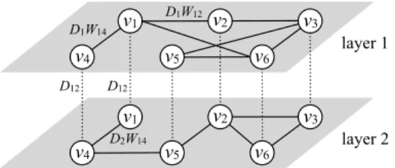
Fig. 2. Strength-biased RW. (a) An original undirected network, whose weighted adjacency matrix is given by A. (b) The modified undirected network,

whose weighted adjacency matrix is given by A′_{. The numbers attached to the edges represent the edge weight. We set}_{α =}_1.

we expect that a node with a large strength tends to have a large p∗

i when

α > −

1 (including for the unweighted case

α =

0) and that the same node tends to have a small p∗

i when

α < −

1. For nodes with a large strength, we expect p

∗

i to increase as

α

increases.

For directed networks in general, one can write a first-order approximation to the stationary density from Eq.(30). We assume that we do not possess any information about the neighbors of

v

i, so we replace p∗j and soutj by their mean values:

p∗_i

=

N

∑

j=1 p∗_j Aji sout j

≈

(const)

×

N

∑

j=1 Aji

∝

sini

.

(35) On both synthetic and empirical networks, Eq.(35)is reasonably accurate in some cases but not in others [126–133].

3.2.3. Relaxation time

To determine the relaxation time to the stationary state, it is instructive to project the solution, Eq. (29), onto an appropriate basis of vectors and to represent it in terms of its modes. The procedure, which is analogous to taking a Fourier transform [see Eq.(2)], is sometimes called a ‘‘graph Fourier transform’’ [134,135] and will be explained in this section [see Eqs.(43)–(45)].

For simplicity, we consider undirected networks. In general, the transition probability matrix T is asymmetric even for undirected networks, except for regular graphs. However, one can derive its eigenvalues and eigenvectors from those of the symmetric matrix

˜

Aij

=

Aij

√

sisj

,

(36) which we can decompose as follows:

˜

A

=

N

∑

ℓ=1

λ

ℓu_ℓu⊤_ℓ

,

(37)

where

λ

_ℓis the

ℓ

th eigenvalue ofA and u

˜

_ℓis the corresponding normalized eigenvector (so that

⟨

u_ℓ

,

u_ℓ′

⟩ =

δ

_ℓℓ′, where

⟨

, ⟩

is the inner product), and

δ

is the Kronecker delta. Because_{A is symmetric, each eigenvalue}

˜

_λ

_ℓ_{is real.}

Because Tij

=

√

sjA

˜

ij

/

√

si, we have the following similarity relationship between T and A [1,136]:

T

=

D−1/2AD

˜

1/2

,

(38) where we defined D (a matrix whose nonzero entries lie only on the diagonal) in Section3.1. Eq.(38)implies that T andA

˜

have the same eigenvalues. In particular, all eigenvalues of T are real-valued, because that is the case forA. The left and right

˜

eigenvectors of T corresponding to the eigenvalue

λ

_ℓare, respectively, uL_ℓ

=

u⊤_ℓD1/2

=

(

(u_ℓ)1

√

s1

, . . . ,

(uℓ)N

√

sN

)

(39) and uR_ℓ

=

D−1/2_u ℓ

=

(

(u_ℓ)1

/

√

s1

, . . . ,

(uℓ)N

/

√

sN

)

⊤

.

(40)

(11)

Using Tn

=

D−1/2A

˜

nD1/2

=

D−1/2 N

∑

ℓ=1

λ

n ℓuℓu⊤ℓD1/2

=

N

∑

ℓ=1

λ

n ℓuRℓuLℓ

,

(41)

we obtain the following mode expansion of the solution of the RW: p(n)

=

p(0)Tn

=

N

∑

ℓ=1

λ

n ℓuLℓ

⟨

p(0)

,

uRℓ

⟩

.

(42) That is, pi(n)

=

N

∑

ℓ=1 a_ℓ(n)(uL_ℓ)i

,

(43) where a_ℓ(n)

=

λ

n_ℓa_ℓ(0)

,

(44) a_ℓ(0)

≡ ⟨

p(0)

,

uR_ℓ

⟩

,

(45) and a_ℓ(n) is the projection onto the

ℓ

th eigenmode. Eqs.(43)–(45)map the state vector p(n), which is defined on the nodes, to a vector (a1(n)

, . . . ,

aN(n)) of eigenvector amplitudes (i.e., their coefficients). This transform, called the ‘‘graph Fourier transform’’, generalizes the standard Fourier transform of an RW [see Eqs.(3)and(7)], and the eigenvectors of the transition-probability matrix T play the role of the Fourier modes eikx_.

For the matrix T andA, the eigenvalues

˜

λ

_ℓeach satisfy

−

1

≤

λ

_ℓ

≤

1 [1,42]. Except in the special cases of multipartite graphs, the strict inequality

λ

_ℓ

> −

1 also holds. In this case, the mode with

λ

_ℓ

=

1 corresponds to the stationary density, and we thus write uL_ℓ

=

p∗

. The right eigenvector that corresponds to this mode is uR_ℓ

∝

(1

, . . . ,

1)⊤. All modes for which

−

1

< λ

_ℓ

<

1 decay to 0. The eigenvalue

λ

_ℓ

=

1 is the largest-magnitude eigenvalue, and the Perron–Frobenius theorem guarantees that all elements of uL

ℓand uRℓare positive. Similar results hold for directed networks, although we cannot take

advantage of the symmetric structure of the matrixA in general. In directed networks, the eigenvalues satisfy

˜

|

λ

_ℓ

| ≤

1. When

|

λ

_ℓ

|

<

1 holds for all but one eigenvalue, which is the case except for directed variants of multipartite graphs with an even number of components, the mode with

λ

_ℓ

=

1 corresponds to the stationary density. In this case, we obtain uL_ℓ

=

p∗

and uR

ℓ

∝

(1

, . . . ,

1)⊤. Again, the Perron–Frobenius theorem guarantees that all elements of uLℓare positive.

By letting n

→ ∞

in Eq.(42), we obtain p∗

=

uL

max

⟨

p(0)

,

uRmax

⟩

, where the subscript ‘‘max’’ indicates the mode

corresponding to the dominant eigenvalue (which is equal to 1). Because uR

max

∝

(1

, . . . ,

1) ⊤

, it follows that

⟨

p(0)

,

uR max

⟩ =

1 regardless of the initial condition p(0). This is consistent with the fact that uL

maxgives the stationary density. By letting n

be large but finite, we obtain

p(n)

≈

uL_max

⟨

p(0)

,

uR_max

⟩ +

λ

n₂uL₂

⟨

p(0)

,

uR₂

⟩

,

(46) where

λ

2 is the second-largest (in magnitude) eigenvalue of T . In deriving Eq.(46), we only kept two terms, because

|

λ

_ℓ

|

n

≪ |

λ

₂

|

nfor all eigenvalues

λ

_ℓwith

ℓ >

2, assuming that

|

λ

_ℓ

|

< |λ

₂

|

(where

ℓ ∈ {

3

, . . . ,

N

}

). Eq.(46)indicates that the second-largest eigenvalue of T governs the relaxation time. More generally, the relaxation speed is determined by the ratio between

|

λ

₂

|

and

λ

max

=

1. The difference 1

−

λ

2is often called the ‘‘spectral gap’’. A large spectral gap (i.e., a

small-magnitude for

λ

2) entails fast relaxation.

The ‘‘Cheeger inequality’’ gives useful bounds on

λ

2[137]. The ‘‘Cheeger constant’’, which is also called ‘‘conductance’’, is

defined by

h

=

min S

{

(number of edges that connect S and S) min

{

vol(S)

,

vol(S)

}

,

(47)

where S is a set of nodes in a network, S is the complementary set of the nodes (i.e., S

∩

S

= ∅

and S

∪

S is the complete set of

the N nodes), and vol(S)

≡

∑

N

i=1;v_i∈Ssi. In the minimization in Eq.(47), we seek a bipartition of a network such that the two parts are the most sparsely connected. (In other words, we want a minimum cut.) The denominator in the right-hand side of Eq.(47)prevents the selection of a very uneven bipartition, which would easily yield a small value for the numerator. The Cheeger inequality is

h2

(12)

so a small Cheeger constant h implies a small spectral gap 1

− |

λ

2

|

and hence slower relaxation. This result is intuitive,

because one can partition a network with a small value of h into two well-separated communities such that it is difficult for random walkers to cross from one community to the other. Note that there are various versions of Cheeger constants and inequalities. They give qualitatively similar – but quantitatively different – results [1,42,54,138–140]. As discussed in Ref. [68] and references therein, such results are important considerations for community detection.

A fact related to the relaxation time is that the power method is a practical method to calculate the stationary density of an RW in a directed network [141]. Suppose that we start with an arbitrary initial vector p(0), excluding one that is orthogonal to p∗

, and repeatedly left-multiply it by T . After many iterations, we obtain an accurate estimate of p∗

. Because any p(0) that is orthogonal to p∗

includes a negative entry, one can start iterations with any probability vector p(0). In practice, one may have to normalize p(n) after each iteration (or after some number of iterations) to avoid the elements of p(n) becoming too large or small.

3.2.4. Exit probability

One is often interested in the probability that a random walker terminates at a particular node, which is then called an ‘‘absorbing state’’. Upon reaching an absorbing state, a stochastic process cannot escape from it. A node

v

iis ‘‘absorbing’’ if and only if Tii

=

1, which implies that Tij

=

0 (for j

̸=

i). A set of nodes is an ‘‘ergodic’’ set if (1) it is possible to go from

v

i to

v

jfor any nodes in the set and (2) the process does not leave the set once it has been reached. An absorbing node is an ergodic set that consists of a single node. A state in a Markov chain is said to be a ‘‘transient state’’ if it does not belong to an ergodic set.

When an RW is composed of N1transient-state nodes and N2absorbing-state nodes, there are N1

+

N2

=

N nodes in

total. Without loss of generality, we relabel the nodes such that

v

1,

. . . , v

N1 are transient and

v

N1+1,

. . . , v

Nare absorbing. The transition-probability matrix T then has the following form:

T

=

(

Q R 0 I

)

,

(49)

where Q is an N1

×

N1matrix that describes transitions between transient-state nodes, R is an N1

×

N2matrix that describes

transitions from transient-state nodes to absorbing-state nodes, and I is the N2

×

N2identity matrix that corresponds to

individual absorbing-state nodes. Taking powers of Eq.(49)yields

Tn

=

(

Qn R

+

QR

+ · · · +

QRn−1 0 I

)

.

(50)

Suppose that we start from transient-state node

v

i and want to calculate the mean number of visits to transient-state node

v

jbefore reaching an absorbing-state node. This number of visits is equal to the (i, j)th element of the matrix

W

=

∞

∑

n=0

Qn

=

(

I

−

Q

)

−1

,

(51) because the (i

,

j)th element of Qn_{is equal to the probability that a random walker starting from}

_v

ivisits

v

jat discrete time

n. The matrix W is called the ‘‘fundamental matrix’’ associated with Q . The matrix on the right-hand side of Eq.(51)is called the ‘‘resolvent’’ of Q . Similar considerations arise in the study of ‘‘central’’ (i.e., important) nodes in networks [142].

The ‘‘exit probability’’ (i.e., the ‘‘first-passage-time probability’’) is defined as the probability Uijthat the walker terminates at an absorbing state

v

jwhen it starts from a transient state

v

i. When there are multiple absorbing-state nodes, it is nontrivial to determine the exit probability. The probability that the walker reaches

v

jafter exactly n steps is given by the (i

,

j)th element of Qn−1_{R. Therefore, we obtain the exit probability in matrix form as follows:}

U

=

∞

∑

n=1

Qn−1R

=

WR

.

(52)

3.2.5. Mean first-passage and recurrence times

When does a random walker starting from a certain source node arrive at a target node for the first time? The answer to this question is known as the ‘‘first-passage time’’ (or ‘‘first-hitting time’’) if the source and target nodes are different and is known as the ‘‘recurrence time’’ (or the ‘‘first-return time’’) when the source and target nodes are identical. Let mij (with i

̸=

j) denote the mean first-passage time (MFPT) from node

v

ito node

v

j. The mean recurrence time is mii. For directed networks, we assume strongly connected networks throughout this section to guarantee that mij

< ∞

(for i

,

j

∈ {

1

, . . . ,

N

}

). For reviews on first-passage problems on networks and other media, see [31,40].

General networks: We first consider some general results. The following identity holds [1,112,113,115]:

mij

=

1

+

N

∑

ℓ=1;ℓ̸=j

(13)

In its first step, a random walker moves from node

v

ito node

v

ℓ, which produces the 1 on the right-hand side of Eq.(53). If

ℓ =

j, then the walk terminates at

v

_ℓ, resulting in a first-passage time of 1. Otherwise, we seek the first-passage from node

v

ℓ(with

ℓ ̸=

j) to node

v

j. This produces the second term on the right-hand side. Note that Eq.(53)is also valid when i

=

j. In matrix notation, we write Eq.(53)as

M

=

J

+

T (M

−

Mdg)

,

(54)

where M

=

(mij), all of the elements of the matrix J are equal to 1, and Mdgis the diagonal matrix whose diagonal elements

are equal to mii. By left-multiplying Eq.(54)by p∗and using p∗J

=

(1

, . . . ,

1) and p∗T

=

p∗, we obtain the mean recurrence time mii

=

1 p∗ i

.

(55)

Eq.(55)is called ‘‘Kac’s formula’’ [1,118,119].

There are several different ways to evaluate the MFPT mij(with i

̸=

j), and it is insightful to discuss different approaches. One method is simply to iterate Eq.(53)[115].

A second method to calculate the MFPT, for a given j, is to rewrite Eq.(53)as

m(j)

=

1

+

T(j)m(j)

,

(56)

where m(j)

=

(m1j

, . . . ,

mj−1,j

,

mj+1,j

. . . ,

mNj)⊤and 1

=

(1

, . . . ,

1)⊤are (N

−

1)-dimensional column vectors and T

(j)

is the (N

−

1)

×

(N

−

1) submatrix of T that excludes the jth row and jth column [124]. The formal solution of Eq.(56)is

m(j)

=

(

L(j)

)

−1

D(j)1

,

(57)

where D(j)is the submatrix of D that excludes the jth row and jth column and L(j)

=

D(j)

−

A(j), where A(j)is the submatrix of A that excludes the jth row and jth column. The matrix L(j)is sometimes called a ‘‘grounded Laplacian matrix’’ [143] (although it is not a Laplacian matrix), and it is invertible because we assumed strongly connected networks. One can derive and solve Eq.(57)separately for each j.

A third method to calculate the MFPT is to take advantage of relaxation properties of RWs [144]. Let pij(n) denote the probability that a walker starting at node

v

ivisits node

v

jafter n moves. The master equation is

pij(n

+

1)

=

N

∑

ℓ=1

piℓ(n)Tℓj

.

(58)

Let Fij(n) denote the probability that the walker starting from

v

iarrives at

v

jfor the first time after n moves. We obtain

pij(n)

=

δ

n0

δ

ij

+

n

∑

n′=0

Fij(n′)pjj(n

−

n′)

.

(59) Using a discrete-time Laplace transform (see, e.g., [145] for an extensive discussion of such generating functions), defined by

ˆ

pij(s)

≡

∞

∑

n=0 e−snpij(n) (60) and

ˆ

Fij(s)

≡

∞

∑

n=0 e−snFij(n)

,

(61) we transform Eq.(59)to

ˆ

pij(s)

=

δ

ij

+ ˆ

Fij(s)p

ˆ

jj(s) (62) and thereby obtain

ˆ

Fij(s)

=

ˆ

pij(s)

−

δ

ij

ˆ

pjj(s)

.

(63)

(14)

Using Eq.(63)then yields mij

=

∞

∑

n=0 nFij(n)

= − ˆ

F ′ ij(0)

=

− ˆ

p ′ ij(0)p

ˆ

jj(0)

+ ˆ

pjj′(0)

[ ˆ

pij(0)

−

δ

ij

]

ˆ

pjj(0)2

.

(64)

To evaluate Eq.(64), we define

R(m)_ij

≡

∞

∑

n=0 nm

[

pij(n)

−

p ∗ j

]

.

(65)

Eq.(65)quantifies the relaxation speed at which pij(n) approaches the stationary density. To write the Laplace transform, we multiply both sides of Eq.(65)by (

−

1)msm

/

m

!

and sum over m. We thereby obtain

∞

∑

m=0 R(m)_ij (

−

1)ms m m

!

=

∞

∑

m=0 ∞

∑

n=0 nm(

−

1)ms m m

!

[

pij(n)

−

p ∗ j

]

=

∞

∑

n=0 e−sn

[

pij(n)

−

p ∗ j

]

= ˜

pij(s)

−

p∗ j 1

−

e−s

.

(66)

Substituting Eq.(66)into Eq.(63)then yields

ˆ

Fij(s)

=

p∗_j s+o(s)

+

∑

∞ m=0R (m) ij (

−

1)m s m m!

−

δ

ij p∗_j s+o(s)

+

∑

∞ m=0R (m) jj (

−

1)m s m m!

=

p ∗ j

+

R (0) ij s

−

δ

ijs

+

o(s) p∗ j

+

R (0) jj s

+

o(s)

=

1

+

R (0) ij

−

R (0) jj

−

δ

ij p∗ j s

+

o(s)

,

(67)

where o(s) represents a quantity that is much smaller than s in the relevant asymptotic limit (s

→

0 in the present case). Consequently, mij

= − ˆ

F ′ ij(0)

=

⎧

⎪

⎨

⎪

⎩

1 p∗ j (j

=

i)

,

R(0)_jj

−

R(0)_ij p∗ j (j

̸=

i)

,

(68)

which is consistent with Kac’s formula [see Eq.(55)]. For undirected networks, substituting p∗

j

=

sj

/∑

N_ℓ=1sℓinto Eq.(68) yields mij

=

⎧

⎪

⎨

⎪

⎩

∑

N ℓ=1sℓ sj (j

=

i)

,

∑

N ℓ=1sℓ sj

(

R(0)_jj

−

R(0)_ij

)

(j

̸=

i)

.

(69)

A fourth method to examine the MFPT is to estimate mijusing a mean-field approximation [146–148]. Regardless of the source node

v

i, the target node

v

jis reached with an approximate probability of p∗j in each time step. Therefore,

mij

≈

∞

∑

n=1 np∗_j(1

−

p∗_j)n−1

=

1 p∗ j

=

mjj

.

(70)

Eq.(70)is a rather coarse approximation, and mijcan deviate considerably from mjj

=

1

/

p∗j. More sophisticated mean-field approaches can likely do better, especially for networks with structures that are well-suited to the employed approximation. There have been many studies of MFPTs for various network models using both analytical and numerical approaches [31,149–153]. We will discuss some examples of undirected and unweighted networks. We focus mainly on the MFPT between different nodes, although it is of course also interesting to calculate recurrence times.

(15)

Regular networks: For a complete graph, mij(with i

̸=

j) is independent of i and j because of the symmetry of the network. Therefore, Eq.(53)reduces to

mij

=

1

N

−

1

+

N

−

2

N

−

1(1

+

mij)

,

(71) which yields mij

=

N

−

1 for i

̸=

j. Kac’s formula [see Eq.(55)] implies that mii

=

N.

For regular lattices Zd_{of any dimension d, Eq.}₍₅₅₎_{implies that m}

ii

∝

N because p∗i

∝

ki

=

2d for any i. Define m•jto be the MFPT averaged over all source nodes

v

i(i

̸=

j) [154]. For Zd, it satisfies the scalings m•j

∝

N2for d

=

1, m•j

∝

N ln N for

d

=

2, and m•j

∝

N for d

=

3.

Erdős–Rényi (ER) random graphs: Consider an ER random graph G(N

,

p), where p denotes the (independent) probability

that each node pair has an edge. Assuming that the mean degree

⟨

k

⟩

is kept constant (i.e., p

= ⟨

k

⟩

/

(N

−

1)

∝

1

/

N), we obtain mii

∝

N and mij

∝

N3/2(with i

̸=

j) as N

→ ∞

[155] for the ‘‘giant component’’ (i.e., a largest connected component that scales linearly with the number N of network nodes as N

→ ∞

[44]). Now suppose that we assume instead that p

>

ln N

/

N,

so that all nodes belong to a single component (in the N

→ ∞

limit) and thus mij(for i

,

j

∈ {

1

, . . . ,

N

}

) is well-defined. It then follows that mijaveraged over all source and target nodes is equal to N

−

1, independently of p [156,157]. In other words, for a sufficiently dense ER random graph, the MFPT is the same as that for the complete graph. The MFPT is much longer for directed ER graphs than for undirected ones, because random walkers do not backtrack on directed networks [158].

Other network models with random features: Much effort in studying RWs on networks has considered first-passage times

on Watts–Strogatz (WS) small-world networks [149,159–164]. As expected, given that WS networks interpolate between regular lattices and ER networks,3 _{these studies have found that the behavior of an RW on WS networks lies somewhere} between that on a regular lattice and that on ER graphs.

Eq.(69)has also been elaborated further for ‘‘scale-free’’ networks, which are defined as networks with a power-law degree distribution p(k)

∝

k−_γ

, where p(k) is the degree distribution. Let us consider scale-free networks that are generated by a ‘‘configuration model’’ [122], so there are no degree–degree correlations. We examine the mean of the MFPT mijover the position of the source node

v

i(with i

̸=

j), which we select according to the stationary density. We usem

˜

•jto denote this weighted mean of the MFPT over i. This mean is distinct from the unweighted mean m•j. For scale-free networks constructed using a configuration model, we obtain for large N that [166]

˜

m•j

∝

⎧

⎨

⎩

N2/ds _(d s

<

2)

,

Nk(1−2/ds)(γ −1) j (2

<

ds

<

2(

γ −

1)

/

(

γ −

2))

,

Nk−_j1 (ds

>

2(

γ −

1)

/

(

γ −

2))

,

(72)

where ds

≡

2df

/

dwis the ‘‘spectral dimension’’ of the network; the ‘‘fractal dimension’’ dfis defined as the exponent of the

scaling relation Nr

∝

rdf, where Nris the number of nodes within distance r from a source node; and the ‘‘walk dimension’’

dwis defined from the scaling relation

⟨

r2

⟩ ∝

t2/dw, where r is the distance between the current position of the walker and

the source node [36,39]. In practice, one calculates the walk dimension as the scaling exponent for the time texitfor a random

walker to exit from a sphere of radius r from the source node (so that texit

∝

rdw) [167]. For regular lattices, dw

=

2, and

the diffusion is thus called ‘‘normal’’. If dw

̸=

2, the diffusion is called ‘‘anomalous’’ [39]. For the ‘‘compact exploration’’ case

of ds

<

2, Eq.(72)suggests that the asymptotic scaling ofm

˜

•jwith N does not depend on the target node at leading order. However, if ds

>

2 (the second and the third cases in Eq.(72)), nodes with higher degrees are reached faster. In particular,

for networks that satisfy the ‘‘small-world property’’ (i.e., the mean path length between nodes scales proportionally to ln N or even more slowly) [165], including popular scale-free network models (such as ones generated by a configuration model), one obtains ds

= ∞

(and dsis very large for many empirical networks). Therefore, the third case in Eq.(72)applies.

Fractal and pseudo-fractal networks: There are various deterministic mechanisms to grow networks in a recursive

manner. Depending on the mode, these algorithms yield ‘‘pseudo-fractal’’ scale-free networks [168] (also called ‘‘hierarchical networks’’ [169,170] or ‘‘transfractals’’ [171]; seeTable 2for different meanings of the term ‘‘hierarchical network’’ that exist in the literature), which have a highly symmetric structure and satisfy the small-world property; fractal networks that do not satisfy the small-world property [171–173]; or classical fractals [39]. These objects are defined and studied in the limit

N

→ ∞

. For such models, it is often possible to exploit their deterministic and recursive nature to exactly calculate the MFPT, and generating functions again can be helpful.

Let us start by looking at fractals that do not have a heavy-tailed degree distribution. In a recursive process of generating a fractal structure from a model of a fractal, we stop the process in each iteration and regard any intersection with more than one edges as a node. In this way, we define a network corresponding to each iteration. The recursive process generates a series of networks, where the number N of nodes becomes larger as one iterates further. We are interested in how the MFPT scales in such networks as a function of N. For example, consider a network constructed from the Sierpinski gasket [177]. When the target node is located at the apex of the gasket, the MFPT averaged over a uniform distribution of the source node is m•j

∝

Nln 5/ln 3

≈

N1.46[39,155,178]. Another example is the so-called ‘‘T-graph’’, which is produced by the initial condition of two nodes connected by an edge and recursive replacement of each edge by a star composed of four nodes

3_{Technically, it is a variant of WS networks with edge rewiring (rather than edge addition) that interpolates between regular lattices and ER}