HAL Id: tel-01624233
https://hal.laas.fr/tel-01624233v2
Submitted on 22 Jan 2019HAL is a multi-disciplinary open access archive for the deposit and dissemination of
sci-L’archive ouverte pluridisciplinaire HAL, est destinée au dépôt et à la diffusion de documents
To cite this version:
Marcus Futterlieb. Vision based navigation in a dynamic environment. Robotics [cs.RO]. Université Paul Sabatier - Toulouse III, 2017. English. �NNT : 2017TOU30191�. �tel-01624233v2�
Contents
1. Introduction 19
1.1. Overview of general robotics context : my point of view of robotics in the
21st century . . . 20
1.1.1. Motivations . . . 20
1.1.2. Ethical analysis . . . 21
1.2. Air-Cobot project . . . 25
1.3. Aims and contributions of this thesis . . . 27
2. Navigation Strategy 29 2.1. Definition of the navigation processes and related works . . . 32
2.1.1. Perception . . . 32 2.1.2. Modeling . . . 33 2.1.3. Localization . . . 33 2.1.4. Planning . . . 34 2.1.5. Action . . . 35 2.1.6. Decision . . . 35
2.2. Description of navigation processes in the Air-Cobot project . . . 36
2.2.1. Air-Cobot platform . . . 36
2.2.2. The Robot Operating System . . . 37
2.2.3. Perception “ exteroceptive” (cameras and lasers) and “propriocep-tive” (odometer) . . . 39
2.2.4. Modeling: both topological and metric maps . . . 43
2.2.5. Absolute and relative localization . . . 45
2.2.6. Planning . . . 55
2.2.7. The action process . . . 55
2.2.8. Decision . . . 63
2.3. Instantiation of the navigation processes in Air-Cobot project . . . 66
2.3.1. Autonomous approach mode . . . 66
2.3.2. Autonomous inspection mode . . . 67
2.3.3. Collaborative inspection mode . . . 68
2.4. General overview about the navigational mode management and modu-larity of the framework . . . 68
2.4.1. Overview of the management of the navigation modes . . . 69
2.4.2. Versatility of the navigation framework . . . 70
2.5. Conclusion . . . 72
3.1.3. Outline of the chapter . . . 79
3.2. Prerequisites of Visual Servoing . . . 79
3.2.1. Robot presentation . . . 79
3.2.2. Robot coordinates system . . . 80
3.2.3. Robot Jacobian and Velocity Twist Matrix . . . 81
3.3. Image-Based Visual Servoing . . . 82
3.3.1. Method . . . 82
3.3.2. Simulation . . . 85
3.4. Position-Based Visual Servoing . . . 92
3.4.1. Method . . . 92
3.4.2. Simulation . . . 94
3.5. Comparison of IBVS and PBVS regarding robustness towards sensor noise on the basis of simulations . . . 101
3.5.1. Simulation conditions . . . 101
3.5.2. The obtained results . . . 102
3.6. The Air-Cobot visual servoing strategy . . . 103
3.6.1. Handling the visual signal losses . . . 105
3.6.2. Coupling the augmented image with the visual servoing . . . 106
3.6.3. PBVS and IBVS switching . . . 106
3.7. Experiments on Air-Cobot . . . 107
3.7.1. Test environment . . . 107
3.7.2. Applying ViSP in the Air-Cobot context . . . 109
3.7.3. Experimental tests combining IBVS with PBVS . . . 109
3.8. Conclusion . . . 117
4. Obstacle avoidance in dynamic environments using a reactive spiral ap-proach 121 4.1. Introduction . . . 122
4.1.1. Air−Cobot navigation environment . . . 122
4.1.2. State of the art of obstacle avoidance . . . 123
4.1.3. Introduction to spiral obstacle avoidance . . . 126
4.1.4. Structure of Chapter . . . 128
4.2. Spiral obstacle avoidance . . . 128
4.2.1. Spiral conventions and definition . . . 129
4.2.2. Definition and choice of spiral parameters for the obstacle avoidance130 4.2.3. Robot control laws . . . 136
4.3. Simulation and experimental results . . . 142
4.3.1. Simulation with static obstacles . . . 142
4.3.2. Experiments in dynamic environment . . . 146
Contents
5. Conclusion 154
5.1. Resume of contributions and project summary . . . 155
5.2. Future work and prospects . . . 156
5.2.1. Addition of a graphic card . . . 157
5.2.2. Using the robot as a platform for autonomous drones . . . 157
5.2.3. Rethink the robot drive system . . . 157
5.2.4. Incorporation of a HUD on a tablet for the operator . . . 158
5.2.5. Real Time capabilities of the platform . . . 159
6. Abstract 162 A. Robot Transformations and Jacobian Computation 166 A.1. Transformations concerning the stereo camera systems . . . 167
A.1.1. Transformation to the front cameras system . . . 167
A.1.2. Transformation to the rear cameras . . . 168
A.1.3. Additional transformations . . . 169
A.2. Kinematic Screw . . . 171
A.3. Velocity screw . . . 175
A.3.1. Solution ”1” of deriving the velocity screw matrix . . . 175
A.3.2. a . . . 175
A.3.3. Solution ”2” of deriving the velocity screw matrix . . . 175
A.3.4. a . . . 176
A.3.5. Applying solution ”2” to our problem . . . 176
A.4. Interaction matrix . . . 178
A.5. Jacobian and Velocity Twist Matrix of Air-Cobot . . . 178
A.5.1. extended . . . 179
A.6. Air-Cobot Jacobian and velocity twist matrix . . . 179
A.6.1. Jacobian - eJe . . . 179
A.6.2. Jacobian- eJe reduced . . . 180
A.6.3. Velocity twist matrix- cVe . . . 180
A.7. Analysis of the Robots Skid Steering Drive on a flat Surface with high Traction . . . 180
A.8. ROS-based software architecture in at the end of the project . . . 182
List of Figures
1.1. Extract of article [Frey and Osborne, 2013]; Likelihood of computerization
of several jobs . . . 22
1.2. Extract of [Bernstein and Raman, 2015]; The Great Decoupling explained 24 1.3. Air-Cobot platform near the aircraft . . . 26
2.1. 4MOB platform and fully integrated Air-Cobot . . . 37
2.2. Remote of the 4MOB platform and tablet operation of Air-Cobot . . . . 38
2.3. Obstacle detection step by step . . . 42
2.4. Example of a navigation plan around the aircraft . . . 44
2.5. Example of a metric map. . . 45
2.6. Example of the absolute robot localization . . . 46
2.7. Example of the VS environment experiments were conducted in . . . 48
2.8. Example of the relative robot localization . . . 49
2.9. 3d model of an Airbus A320 that was used for matching scans acquired for pose estimation in the aircraft reference frame (red = model points / blue = scanned points) . . . 51
2.10. Example of two scans that were acquired with an Airbus A320 in a hangar environment . . . 52
2.11. Transformations during ORB-SLAM initialization . . . 53
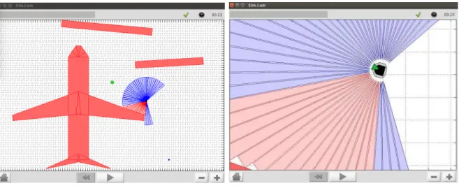
2.12. Simulator that helped in the evaluation of new, rapidly prototyped ideas throughout the Air-Cobot project . . . 57
2.13. Basics of the mobile base angular velocity ω calculation. . . 58
2.14. Adjustment to the standard go-to-goal behavior . . . 58
2.15. Aligning first with a target ”in front” and ”behind” the robot . . . 59
2.16. Modification of the align first behavior to decrease tire wear. . . 61
2.17. Correct-Camera-Angle controller . . . 62
2.18. Picture of Air-Cobot in default configuration and with the pantograph-3d-scanner unit extended for inspection . . . 64
2.20. Schematic of the state machine which defines the decision process . . . . 64
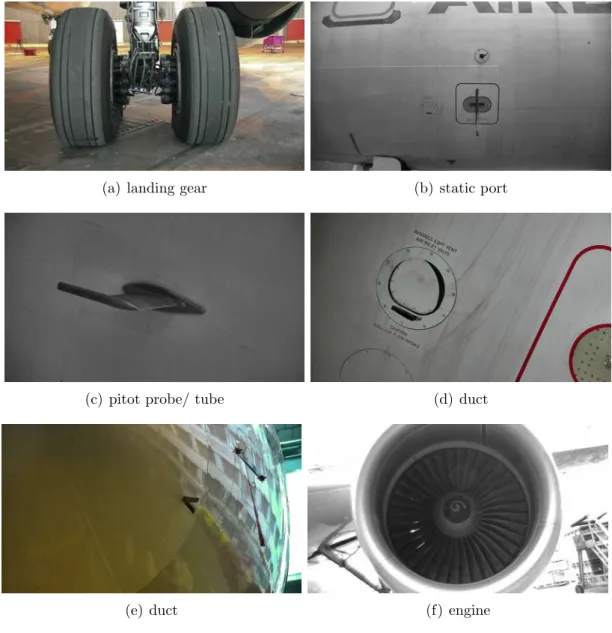
2.19. Collection of elements that are inspected in a pre-flight check . . . 65
2.21. A general overview of the high level state machine of Air-Cobot . . . 69
2.22. Building costmaps with the help of the ROS navigation stack . . . 71
2.23. Costmaps build during the experiment . . . 72
3.1. Air-Cobot and the associated frames [Demissy et al., 2016] . . . 80
3.2. Robot coordinate system for the front cameras [Demissy et al., 2016] . . 80
3.3. Projection in the image-plane frame . . . 83
3.8. Evolution of the visual error in a IBVS simulation . . . 91
3.9. Evolution of velocities in a IBVS simulation . . . 92
3.10. Block diagram for the PBVS approach . . . 94
3.11. Evolution the point C (camera origin) in a PBVS simulation . . . 96
3.12. Evolution of features in a PBVS simulation . . . 97
3.13. Robot path, orientation and camera state in a PBVS simulation . . . 97
3.14. Evolution of error in a PBVS simulation . . . 98
3.15. Evolution of velocities in a PBVS simulation . . . 99
3.16. Evolution the point C (camera origin) in a noisy simulation . . . 102
3.17. Evolution of features in a noisy simulation . . . 103
3.18. Robot path, orientation and camera state in a noisy simulation . . . 104
3.19. Evolution of error in a noisy simulation . . . 104
3.20. Evolution of velocities in a noisy simulation . . . 105
3.21. Example of the lab environment where the visual servoing experiments were conducted in . . . 108
3.22. Extract of video sequence showing an outside view onto the experiment . 110 3.23. Extract of video sequence showing the system handling switching between IBVS and PBVS . . . 111
3.24. Position and velocity (linear and angular) plots obtained during the IBVS-PBVS combination experiment . . . 112
3.25. Orientation and velocity plots obtained during the feature loss experiment 113 3.26. Extract of video sequence showing the systems capability to handle fea-ture loss during execution of a visual servoing-based navigation mission . 115 3.27. Outline of the Gerald Bauzil room in which the experiment takes place with expected path for the robot . . . 116
3.28. Extract of video sequence showing the systems capability to perform a combination of IBVS-PBVS-Metric based navigation . . . 118
4.1. Dealing with airport forbidden zones . . . 123
4.2. Moth flight path being ”redirected” by an artificial light source . . . 127
4.3. Spiral Concept as presented in [Boyadzhiev, 1999] . . . 128
4.4. Spiral conventions for an ideal case . . . 129
4.5. Three schematics of spiral obstacle avoidance patterns . . . 130
4.6. Spiral convention in a real life situation . . . 132
4.7. Target and Obstacle Schematics . . . 134
4.8. Visualization of spiral obstacle avoidance extension for moving obstacles . 135 4.9. Graph visualizing relationship between eξ and αd (blue,uninterrupted line ֒→ Air−Cobot configuration) . . . 136
4.10. Real life robot model with application point for control inputs . . . 137
List of Figures
4.12. λ as a function of the angular error eα . . . 139
4.13. Visualization of the first draft for the SOM determination . . . 140
4.14. Visualization of SOM determination . . . 140
4.15. Example of when to overwrite obstacle avoidance. . . 142
4.16. Extract of video sequence [Futterlieb et al., 2014] - static obstacles . . . . 143
4.17. Proof of Concept of an outwards spiraling obstacle avoidance . . . 144
4.18. Avoidance Experiment for static Obstacles . . . 145
4.19. Robot linear and angular Velocities and Camera Angle . . . 149
4.20. Extract of video sequence - static obstacles . . . 150
4.21. Extract of video sequence - dynamic obstacles (a) . . . 151
4.22. Extract of video sequence - dynamic obstacles (b) . . . 152
4.23. Robot trajectory. . . 152
4.24. Successive robot positions - Close up of first OA . . . 153
4.25. Linear and angular velocities . . . 153
4.26. eξ . . . 153
5.1. Sketch and cross section of the Mecanum wheel [Ilon, 1975] . . . 158
5.2. Heads Up Display for mobile devices for Air-Cobot control designed by 2morrow . . . 159
A.1. Robot coordinate system for the front cameras . . . 167
A.2. Robot coordinate system for the rear cameras . . . 169
A.3. Robot Coordinate System . . . 170
A.4. Aircobot Dimensions . . . 178
A.5. Graph showing all nodes that run during a navigation mission . . . 182
A.6. Extract of PTU datasheet [man, 2014] . . . 183
List of Algorithms
2.1. Obstacle Detection Algorithm . . . 41
2.2. 3D Point Cloud Matching . . . 50
2.3. Modified RANSAC . . . 50
2.4. Modified Align First Behavior . . . 60
3.1. Algorithm that determines the stop of position-based visual servoing . . . 100
4.1. Checklist for OA . . . 137
4.2. Decision tree for choosing SOM . . . 141
List of Tables
2.1. Description of the navigation strategy during the approach phase . . . . 67
2.2. Description of the navigation strategy during the autonomous inspection phase . . . 68
2.3. Description of the navigation strategy during the collaborative phase (Fol-lower mode) . . . 68
3.1. Parameters of the IBVS simulation . . . 88
3.2. Parameters of the PBVS simulation . . . 96
3.3. Parameters of the IBVS/PBVS comparison . . . 102
Abbreviations
AI Artificial Intelligence
CPU Central Processing Unit
d Dimensions/dimensional
DARPA Defense Advanced Research Projects Agency
DWA Dynamic Window Approach - A planner able to deal with
obstacles locally
DOF Degree of Freedom
FOV Field Of View
Gazebo Simulator general suggested for working on ROS
GPU Graphic Processing Unit
IBVS Image-based Visual Servoing
ICP Iterative Closest Point
IMU Inertial Measurement Unit
Laser Light amplification by Stimulated Emission of Radiation
LRF Laser Range Finder
NDT None-Destructive Testing
OA Obstacle Avoidance
PBVS Position-based Visual Servoing
PTU Pan-Tilt-Unit
PTZ Pan-Tilt-Zoom camera
RANSAC RANdom Sample Consensus
RANSAM RANdom Sample Matching
ROS Robot Operating System - Software allowing a simple
inte-gration of hardware and some off the shelf functionality for robots - For more information seeking Section 2.2.2 on Page 37
Intelligent Systems (GRITS) Lab (see [de la Croix, 2013]
SLAM Simultanious Loclaization And Mapping
SNR Signal to Noise Ratio
SVO Semi-Direct Visual Odometry - A visual odometry proposed
by members of the Robotics and Perception Group, University of Zurich, Switzerland
TEB Timed Elastic Band - In order to avoid high level re-planning
this approach allows for local path deformation in order to avoid obstacles
ViSP Software package loosly based on OpenCV that allows a
rela-tively simple and rapid visual servoing implementation - De-veloped by INRIA
1. Introduction
Contents
1.1. Overview of general robotics context : my point of view of
robotics in the 21st century . . . 20
1.1.1. Motivations . . . 20
1.1.2. Ethical analysis . . . 21
1.2. Air-Cobot project . . . 25
1.3. Aims and contributions of this thesis . . . 27
1. A robot may not injure a human being or, through inaction, allow a human being to come to harm.
2. A robot must obey the orders given it by human beings, except where such orders would conflict with the First Law.
3. A robot must protect its own existence as long as such protection does not conflict with the First or Second Laws.
[Asimov, 1950]
the contemporary advancements in autonomous driving, surgical or surveillance robots [Marquez-Gamez, 2012] we can safely assume that the amount of robots that will find their way from the research labs to our everyday life is increasing, whether we are afraid of this development or we embrace it. These robots mainly belong to the domain of mobile robotics which encompasses a vast range of terrestrial vehicles, underwater and aerial robots (Unmanned Aerial Vehicles, UAV’s) [Marquez-Gamez, 2012].
From time to time they still remind us of kids that need our help to understand their surroundings but with each passing year their algorithms become more and more mature. Just one look at the DARPA challenge for robotics shows us how far technology has come in recent years. Thinking about the Urban Challenge [Eledath et al., 2007], [Balch et al., 2007], [McBride, 2007] and looking at the maturity of self driving cars in 2017, this becomes even more obvious. It is very unlikely that this trend is going to change. If anything, the speed at which new technologies will be introduced will just increase.
As humans we are very versatile and quickly learn how even the most complex tasks can be performed. However, it still happens that we make mistakes in particularly stress-ful situations. These situations are encountered in aviation domain where a lot of studies on ”human risk factors” have been conducted [Degani and Wiener, 1991], [Latorella and Prabhu, 2000], [Maintenance, ], [Drury, 2001] and [Shappell and Wiegmann, 2012]. The risk can be reduced by designing ”fool-proof” checklists, increasing the amount of R&R (Rest and Recuperation) of the staff or in some cases even double checking by a sep-arate inspector [Rasmussen and Vicente, 1989], [Latorella and Prabhu, 2000]. A new trend is to help or to assist the staff in their daily tasks by robots. Taking a look at
popular Utopian (and sometimes even Dystopia) fiction [Asimov, 1950], [ ˇCapek, 2004],
partly even [Lem, 1973] and [Dick, 1982], humans work force is completely replaced by machines. These developments then present a huge challenge to society and are meant as a warning to question technological progress. It is here, where humanity’s challenge will lie in the future. How we will deal with the ever declining amount of blue collar and (more and more so) white collar jobs [[email protected], 2014].
Another trade that we share as a species is that believe that technological progress advances in a linear fashion. If asked what kind of technologies will be introduced in the next five to ten years, we will take a look back at where we were five to ten years ago and make a linear extrapolation of what there is to come. This perception of linear progress however is flawed, because every new invention or discovery allows us to ad-vance faster. Hence the technological change is exponential [Kurzweil, 2004], [Kurzweil,
1. Introduction
2005], [Kurzweil, 2016]. This fact alone shows that the future is exciting, however, we should not follow technological advance blindly. Human history is full of examples where an invention’s potential for bad was underestimated until it was too late. This of course does not mean that certain progress in technology can be stopped, however, it might be worth the time to consider (and anticipate) the consequence of our work. For instance, the mere prospect of a world without the need for manual labor, dangerous or dull work-ing conditions does not make it a world worth livwork-ing in. We will have to shape it so that all of human kind can profit from it, because if we continue like we have only very few people will get the luxury of living their life in a truly Utopian world, while the rest will struggle to survive. To go further into detail the next section will give a short ethical analysis about this statement.
1.1.2. Ethical analysis
In the previously mentioned science fiction novels, the narrator never fails to show us the dangers that comes with these improvements to technology. So, as we are taking further steps on a path that was so beautifully lain down in front of us, we should always keep in mind that we are not flawless and therefore, step ahead with care.
In this short paragraph, I would like to reflect on the ramifications and consequences of the replacement of human workers by machines. We want to focus this ethical analysis on the consequence of this on the employment market, since for most adults, a rather great time is spent working.
People have always been scared of new technology that might reduce the amount of available jobs (invention of printing, steam machine, etc.), but history has shown us that in fact, jobs that were destroyed have been compensated for (in some cases even exceeded) by sparking an era of growth due to the technological advance. Therefore, this mistrust and resistance towards new technology is not a recent development. However, in the past few years a discussion among scientists has started about how the robot revolution is fundamentally different to all the previous changes mankind has seen so far (Gutenberg printing press, steam machine, industrial revolution, etc.) and which in the long run have created more jobs than were destroyed [Frey and Osborne, 2013], [Brynjolf-sson and McAfee, 2014], [[email protected], 2014], [Ford, 2015]. If before the concern was mostly focused on the disappearance of low-skilled jobs and could be countered by the creation of new areas of employment, our society will be faced with robots competing for high-skilled jobs as well.
Figure 1.1 shows an extract form [Frey and Osborne, 2013] in which the likelihood of automation of specific jobs in the upcoming two decades is given. More and more scientists have come to realize that one of the hardest challenges for human kind might not be connected to satisfying basic needs, such as shelter, hunger etc. (although we are far from eradicating those needs at the moment), but might actually be associated with providing proper reason and purpose to our existence.
Figure 1.1.: Extract of article [Frey and Osborne, 2013]; Likelihood of computerization of several jobs
A more advanced illustration of this concept “robots replace human” was shown on the example of general practitioners and the cognitive computer system “Watson” by IBM in the popular video “Humans Need Not Apply” of CGP Grey [[email protected], 2014]. “Watson” can be considered as an Artificial Intelligence, AI, developed by International Business Machines Corporation, IBM, in DeepQA project. The software is capable of understanding and answering questions that are posed in natural language (as opposed to a well structured data set), which is the form most information exist today. For the purpose of demonstration “Watson” was developed to challenge human participants in the popular quiz show Jeopardy!. By having access to four terabytes of structured and unstructured information (including the full text of Wikipedia) Watson was able to defeat former winners Brad Rutter and Ken Jennings in 2011 [Wikipedia, 2015]. In recent years Watson was also tested in medical field of oncology [Malin, 2013], [Strick-land and Guy, 2013]. Watson was able to show its potential in this field because of its fast pattern recognition among extremely big data sets that can not be processed by any human physician. And although the AI is still far from perfect, this example shows that it is not only the blue colored jobs that might be replaced (or reduced) by machines. In fact, Watson does not need to be perfect, it just needs to be better than its human counterpart. [Ferrucci et al., 2013] is referring to reports that diagnosis error
1. Introduction
outnumber other medical errors by far. The main causes for those is thought to be the fast growing amount of new medication and research that no physician can keep up with during the working week. An AI with an advanced pattern recognition such as Watson completes this work much quicker. Furthermore, any miss-diagnosis by the machine will improve the next diagnosis. This might also be the case for the human counterpart, however, here it will only be the patients of that particular physician that will profit from his/her learning expertise. Patients of another doctor might suffer the same miss-diagnosis [[email protected], 2014]. Studies have shown that certain physicians would need to read up to 627 hours [Alper et al., 2004] per month (consisting of papers and information about the latest medication, side effects and other research results) in order to keep up with the ever growing amount of available information about medication. It is unlikely that this number will decrease in the future. In fact, it is far more reason-able to assume that the amount of availreason-able medication, and therefore, the amount of possible side effects will only increase.
This leads us to the main problem. There are certain areas (automation, pattern recognition, etc.) in which a human will most likely not be able to beat its computer counterpart in the upcoming decades. And if the machine actually does provide better results, who would stop patients of seeking out its advice? And what will we do with the millions of people that will fall into unemployment because of automation? Who will provide for their financial security? This is not a problem that lies in the far future. According to [Bernstein and Raman, 2015], Brynjolfsson states that since the 1980s, the median income has begun to shrink. In Figure 1.2, we can see this trend that shows a nearly constant increase in labor productivity which had been followed by an equivalent increase of median family income until these trends began to separate in the 80s. Brynjolfsson fears that due to more and more automation this problem will get worse. Even more dangerous is the fact that the private employment seems to have stagnated in the 2000s although even though the economy has not. These two developments are what Brynjolfsson and McAfee refer to as the ”Great Decoupling”. He further states that a decrease of income equality has been registered throughout developed countries world-wide in the past 30 Years.
I personally believe that there is no simple answer to this problem. Keeping Moore’s law [Moore, 1965] in mind even a very conservative person will have to accept that we will face more and more automation in the years to come. Of course we could try to prevent the rapid increase of automation. However, looking at technological advances throughout history, it will be hard (or even impossible) to find a case where this approach ever worked.
As we have stated before, throughout history, parts of the human population have always fought against technological advancement. Mainly, because they saw that their jobs were threatened. In retro-spec we can see that their jobs really were eradicated, however, due to the new technology (which they formerly had fought against), a com-pletely new and at most times better (health risks, payment, etc.) line of work was
Figure 1.2.: Extract of [Bernstein and Raman, 2015]; The Great Decoupling explained created. It is a fact that this opinion was the shared consensus among scientist for many years. Basically assuming that the problem would solve itself.
However, even in the research community more and more scientist claim that the amount of jobs being replaced by machines and software can not match the amount of new jobs that are being created at the same time. In fact, since one of the main drives for innovation in human society has always been optimization and increasing the effectiveness of processes in order to increase the profit (industrialization, green revolution, robotics) it is actually not surprising that we are succeeding in eradicating the need for human workforce more and more. In the end, was that not the idea in the first place? We forgot however, that the current system we live in is not a welfare system in which only a few people have to work. On the contrary, some of the most industrialized, first world countries become more and more anti-social. Recent polls show that more half of the American (USA) working population is in fact struggling to earn a living. [Online, 2016] states that the median US American worker received less than 30k $ net payment in the year 2014. This while many of these people are actually working more than one job. The wealth gap is increasing and more automation might just accelerate this trend.
If the system is not changed, those people will be the first ones without a job, without social security, without health care and retirement money. We should be careful not to dismiss these concerns and just hope that somehow enough paying jobs will survive the automation revolution. There is however and upside to this. If we look around in our communities, it is hard to get the impression that there is not enough work for everyone.
1. Introduction
Sure, there might not be enough paid work, but there is enough to do. Additionally, of those people that do have a paid job, it is hard to find someone that is not forced to work more and more. The effect of such an employment is often that the employee is becoming unsatisfied that thinks beside work are not taken care of as much as he / she would like. Personally, I believe that this is exactly the upside of the problem. There is enough work, we just need to find a way to change the system we are living in to support people in doing it.
1.2. Air-Cobot project
Air-Cobot project is not an example of extreme automation of human tasks, as the “cobot” is expected to help the staff in hard working conditions rather than to replace it. It takes place in the aeronautical context to improve the safety of passengers and optimize the maintenance of aircraft.
There are nearly 100,000 commercial flights per day, which means that one thousand of aircraft inspections per hours occur across the globe. However, 70% of the inspections are still conducted visually by co-pilots and maintenance operators, which increase aircraft down-time and maintenance costs. In addition, these inspections are performed whatever the weather (rain, snow, fog, ...) and the light conditions (day, night).
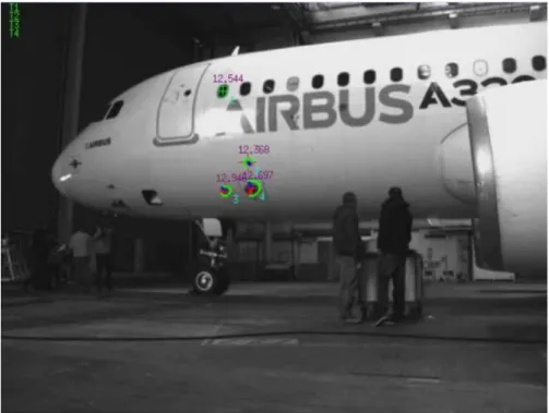
The Air-Cobot is therefore a collaborative robot that automates visual inspection procedures. It helps co-pilots and maintenance operators to perform their duties faster, more reliably with repeatable precision. The robotic platform can provide a great and valuable help when the inspections conditions become tricky. Our main objective in this project is then to achieve a collaborative pre-flight inspection of an aircraft between the co-pilot or the operator and a robot. This latter must be able to navigate alone around the aircraft between the twenty different check points, while preserving the safety of the workers which are around the aircraft and the cars or trucks which are on the refueling area.
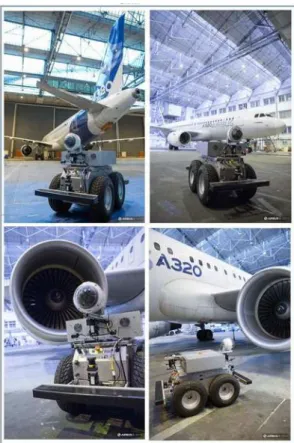
During the pre-flight inspection, the robot receives a maintenance planning from a human operator monitoring which aircraft is ready to be inspected. With this plan, the robot starts the navigation from its charging station towards the inspection area. During the approach to the test side, the robot moves along dedicated roads which are free obstacles corridors. Whenever the inspection area is reached, the aircraft can be detected and the robot moves relatively to it with respect to the maintenance planning. While performing the inspection task, the robot constantly sends progress reports to the flight personal and a trained operator. This latter will then be able to help out in case the robot encounters obstacles that block a checkpoint, malfunction in its sensors or similar unpredictable problems. When the Air-Cobot has finished its task to the operators satisfaction, it moves on to the next mission or navigates its way back to the charging station. Figure 1.3 shows the robot during an inspection task conducted in the
Figure 1.3.: Air-Cobot platform near the aircraft early 2015 at the Airbus site Toulouse-Blagnac with an Airbus A320.
As shown in Figure 1.3, the robot is a 4MOB platform designed by STERELA. It consists of four independent wheels which are controlled in velocity. Additionally, it is outfitted with numerous navigation sensors : an IMU and a GPS; 2 stereo camera systems mounted on a pan tilt unit (PTU); a pan tilt zoom camera (PTZ); a laser range finder (LRF). More details about the robot and its sensors are provided in the upcoming chapter (see Section 2.2 on Page 36).
The robot is then endowed with all the necessary sensors allowing to implement the navigation modes. Indeed, three main navigation modes / phases can be highlighted :
• “ an autonomous approach phase ”, where the robot goes from the charging station to the aircraft parking area following a dedicated shipping lane. Thus, to fulfill its mission, the robot has to perform a large displacement along the road, as the initial and final points might be far. The airport environment is a highly constrained environment where the displacements obey precise rules. Thus a priori information will have to be given to the robot in order to avoid any forbidden path. As a conclusion, the approach phase from the charging station to the aircraft parking area needs an absolute navigation following a previously learnt path.
1. Introduction
• “ an autonomous inspection phase ”, where the robot moves around the aircraft throughout a cluttered environment. The approach needs a large displacement with a highly efficient obstacle avoidance to respect strong security requirements. The navigation is mainly based on a relative navigation to the aircraft while taking into account the obstacles (aircraft, vehicles, maintenance or flight crew, etc.). • “ a collaborative inspection phase ”, where the robot follows the co-pilot or a
maintenance operator. Here, the autonomy of the robot is reduced, as the motion is defined by the person in charge of the pre-flight inspection.
The two first above mentioned navigation phases are at the core of my research work.
1.3. Aims and contributions of this thesis
This PhD work focuses on multi-sensors based navigation in a highly dynamic and cluttered environment. To answer this problem, we have tackled the following issues :
• long range navigation far and close to the aircraft, • obstacle avoidance,
• appearance and disappearance of the aircraft in the image, • integration on a robotic platform.
To deal with the above mentioned problems, a navigation strategy needed to be de-veloped. This strategy makes use of the sensors (GPS/vision/laser) which are the most appropriate depending on the phase and on the situation the robot is. In order to be able to navigate far and close to the aircraft, it is necessary that our strategy features local and global properties. The navigation problem is analyzed first, from a general point of view, highlighting the different processes which are at its core: perception, modeling, planning, localization, action and decision. Our first contribution consists in the instantiation of these processes to obtain the desired global and local properties. Here is a brief overview of the instantiated processes before a more detailed explanation will follow in the subsequent chapters. Perception is both based on “exteroceptive” and “proprioceptive” sensors. Detection and tracking algorithms have also been developed to control the robot with respect to the aircraft and to avoid static and dynamic obsta-cles. The modeling process relies on a topological map (the sequence of checkpoints to be reached) and two metric maps. Here the first one is centered on the robot last reset point and the second one on the aircraft to be inspected. A data fusion technique is also suggested for the relative localization of the robot versus the aircraft. The action process is made of several controllers allowing to safely navigate through the airport. The decision process allows to monitor the execution of the mission and to select the best controller depending on the context.
high accuracy demand, the visual servoing controller will always be used as the primary means to reach the target. We will then compare different solutions to determine which of the different visual servoing controllers is the most optimal adapted to the current situation. In addition, we have also taken into account the problem of visual signal losses which might occur during the mission. We then propose a combination of both Image-based and Position-based visual servoing in a framework that: (i) reconstructs the features if they disappear with the help of a virtual image which is updated online with several sensors used simultaneously ; (ii) is able to find back these features ; and (iii) even navigate using only their reconstructed values. Finally, it is important to note that the Air-Cobot platform is equipped with five cameras, leading to a multi-visual servoing control law.
Our third contribution is related to obstacle avoidance. It is performed with the help of a laser based controller which is activated as soon as dangerous objects are detected. This reactive controller allows to avoid both static and dynamic obstacles. It relies on the definition of an avoidance spiral, which can be modified online depending on the needs (newly detected obstacles, path free anew, mobile objects motion, etc.). We will show that this approach (which is based on the flight path of insects) is extremely reactive and can be well adapted to the task at hand.
Finally, all these contributions are integrated on a robotic prototype that was designed solely for the purpose of the proof of concept which is the underlying task in the Air-Cobot project and this thesis. A framework that can communicate with the robotic platform, all its sensors and two different PC’s was developed during the course of this thesis. At the heart a Linux system running a ROS-Hydro distribution will allow the navigational supervisor module to choose the best controller for every situation the robot can find itself in.
This manuscript is organized as follows. The next three chapters are dedicated to the three above mentioned contributions. All the described methods are validated by simulation and experimentation results. The experimental tests have been conducted either in LAAS or in Airbus Industries site in Blagnac. Finally, a conclusion ends this work and highlights the most promising prospects.
2. Navigation Strategy
Contents
2.1. Definition of the navigation processes and related works . . 32 2.1.1. Perception . . . 32 2.1.2. Modeling . . . 33 2.1.3. Localization . . . 33 2.1.4. Planning . . . 34 2.1.5. Action . . . 35 2.1.6. Decision . . . 35 2.2. Description of navigation processes in the Air-Cobot project 36 2.2.1. Air-Cobot platform . . . 36 2.2.2. The Robot Operating System . . . 37 2.2.3. Perception “ exteroceptive” (cameras and lasers) and
“propri-oceptive” (odometer) . . . 39 2.2.4. Modeling: both topological and metric maps . . . 43 2.2.5. Absolute and relative localization . . . 45 2.2.6. Planning . . . 55 2.2.7. The action process . . . 55 2.2.8. Decision . . . 63 2.3. Instantiation of the navigation processes in Air-Cobot project 66 2.3.1. Autonomous approach mode . . . 66 2.3.2. Autonomous inspection mode . . . 67 2.3.3. Collaborative inspection mode . . . 68 2.4. General overview about the navigational mode
manage-ment and modularity of the framework . . . 68 2.4.1. Overview of the management of the navigation modes . . . . 69 2.4.2. Versatility of the navigation framework . . . 70 2.5. Conclusion . . . 72
can be divided into three main modes / phases. Those three phases will be presented in the following and will be mentioned throughout this work:
• “ an autonomous approach phase ”, in which the robotic platform moves from charging station to aircraft parking area (inspection side) following a dedicated lane for autonomous vehicles on the airport. Hence, to fulfill its mission, the robot has to perform a large displacement along that lane, as the initial and final points might be far apart from each other. In addition, the space to be crossed is rarely cluttered with obstacles because it is dedicated for the robot alone. However, a contingency plan has to be put in place. One thing that simplifies the task at hand is that an airport is indeed a highly structured / constrained environment. This results in a large amount of a priori available informations which can be merged into metric maps or can be taken into consideration when designing topological maps. Thus a priori information will have to be given to the robot in order to avoid any forbidden path.
• “ an autonomous inspection phase ”, where the robot moves relative to the aircraft throughout a cluttered environment. To perform this mission, the robot will have to reach each checkpoint that was chosen specifically for each aircraft type robustly and successively. During this phase, a large displacement, due to the size of the aircraft, has to be realized. Borrowing from the concept of “ Divide and Conquer ” this large displacement is made of small partially independent motions. In addi-tion, strong security requirements have to be considered, as the robot must avoid any obstacle present in its surroundings (namely: the aircraft, various transport vehicles, maintenance or flight crew, forbidden fueling zones, etc.). During this phase the robot will remain in relative close vicinity of the aircraft since it sym-bolizes its main means of self-localization. This particular phase also represents the main proof of concept scenario for the Air-Cobot project.
• “ a collaborative inspection phase ”, where the robot follows the co-pilot or a maintenance operator. Here, the autonomy of the robot is reduced, as the motion is defined by the person in charge (called the operator from here on out) of the pre-flight inspection. However, the full band of security functions is still needed. Even though the operator by him / herself represents an obstacle it is necessary for the robotic platform to still consider other objects that might cross the virtual tether. Furthermore, a tracking is essential to prevent false object following, meaning, that the half silhouette of the operator must be kept during this phase at all times. The PhD thesis at hand is mainly focused on the two first modes / phases for which a high level of autonomy is required. To achieve the considered challenge it is
neces-2. Navigation Strategy
sary to define an efficient navigation strategy able to perform long displacements while guaranteeing non-collision, both in a large spaces as in close vicinity to the aircraft. Ad-ditionally, the proposed strategy needs to work in very different environments, typically on aircraft tarmac as well as in hangars. To gain further insight into the challenges, the next paragraph will review the state of the art on this general subject.
In robotics literature, it is common practice to divide the navigation strategies into two main groups [Choset et al., 2005, Siegwart and Nourbakhsh, 2004, Bonin-Font et al., 2008]. A first group which bundles approaches in need of extensive a priori knowledge is usually referred to as “global approach”. In other words, if the robot does not receive
a map about its environment prior to the mission, it cannot start 1. It then “ suffices
” to extract and follow a path connecting the initial position to the goal to perform the task. This approach is suitable to realize large displacements because it offers a global view of the problem. However, it suffers from well-studied drawbacks: mainly, a lack of flexibility when dealing with unmapped obstacles, some sensitivity in the pres-ence of errors (especially if metric data are used to build the map or to localize the robot), etc. From this information alone the analysis for the Air-Cobot project is that global strategies could be well adapted to perform the “ autonomous approach phase ”. Indeed, during this phase, the environment must be precisely described to the robot to avoid forbidden paths defined on the airport. Hence, a dedicated pre-navigation step using a SLAM technique then appears mandatory. SLAM, which is the acronym for Simultaneous Localization And Mapping, is a well known approach to generate metric information about the system environment while continuously performing a self localization in the metric data. As previously mentioned, the charging station might be far from the aircraft parking / inspection area, forcing the robotic platform to perform a long-range displacement, thus, increasing the interest of this approach in our context. However, let us note that it might be challenging to avoid unmapped obstacles with this kind of approach.
The second group, called “local approach”, mostly covers reactive techniques which do not require a large amount of a priori knowledge about the environment. The robot then moves through the scene depending on the goal to be reached and on the sensory data gathered during the navigation. These techniques allow to handle unexpected events (such as non mapped obstacles for instance) much more efficiently than the group of approaches described before. However, as no (or insufficient) global information is available, they are not well suited to perform long displacements. Hence, this approach seems to be more appropriate to implement the “ autonomous inspection ” during which the robot has to move relatively about the aircraft. Indeed, during this step of the
mission, it will be necessary to avoid many unpredictable obstacles2, either static (fuel
or baggage trucks parked in the aircraft vicinity, fuel pipes, etc) or mobile (moving 1
The map can be built either by the user or automatically during an exploration step.
2
Remember that even though the robot is developed for the well structured environment of an airport, a contingency plan needs to be put in place for all probable eventualities.
aircraft size, it appears that a long-range displacement might be necessary to perform the preflight inspection. This is one of the main challenges to overcome while designing our strategy. Therefore, it is clear that the desired navigation strategy must integrate both local and global aspects to benefit from their respective advantages. For the mission at hand both approaches are complementary and the strategy must be built to take this characteristic into account. To do so, we propose an initial analysis of the problem at a lower level and we split the navigation system into the six following processes: perception, modeling, planning, localization, action and decision. All involved processes can be instantiated depending on the needs of each navigation mode. The current chapter aims to answer the following question: “How can the processes be instantiated accordingly to the embedded sensors and the navigation modes? ”
To propose a suitable response to this question, a general review of the navigation processes is first presented before showing how they have been instantiated to fulfill the requirements of the Air-Cobot project.
2.1. Definition of the navigation processes and related
works
The following section is devoted to the description of the processes involved in the naviga-tion. As mentioned earlier, a total of six processes are generally highlighted: perception, modeling, planning, localization, action and decision. A wide range of techniques are available in the literature for each of them. As these processes cooperate within a frame-work to perform the navigation, they cannot be designed independently and an overview of the problem is required to select the most suitable among different available methods. We present here-below such an overview.
2.1.1. Perception
In order to acquire the data needed by the navigation module, a robot can be equipped with both “ proprioceptive ” and “ exteroceptive ” sensors. While the first group of sensors (odometers, gyroscopes, . . . ) provide data relative to the robot internal state, sensors of the second group (camera, laser telemeters, bumpers, . . . ) give information about its environment. The sensory data may be used by four processes: environment modeling, localization, decision and robot control.
2. Navigation Strategy
2.1.2. Modeling
A navigation process generally requires an environment model. This model is initially built using a priori data. It cannot always be complete, and might evolve with time. In this case, the model is updated with the help to data acquired during the navigation. There exists two kinds of models, namely the metric and/or topologic maps [Siegwart and Nourbakhsh, 2004].
The metric map is a continuous or discrete representation of the free and occupied spaces. A global frame is defined and robot with respect to obstacles poses are known with more or less precision in this frame. The data must then be expressed in this frame to update the model [Choset et al., 2005].
The topologic map on the other hand is a discrete representation of the environment based on graphs [Choset et al., 2005]. Each node represents a continuous area of the scene defined by a characteristic property. All areas are naturally connected and can be limited to a unique scene point. Characteristic properties, chosen by the user, may be the feature visibility or its belonging to a same physical space. Moreover, if a couple of nodes verifies an adjacency condition, then they are connected. The adjacency condition is chosen prior to the mission execution by the user and may correspond for example to the existence of a path allowing to connect two sets, each of them represented by a node. A main advantage of topologic map is their reduced sensitivity to scene evolution: a topologic map has to be updated solely if there are modifications concerning the area represented by the nodes or the adjacency between two nodes. This is extremely helpful for the project at hand since the aircraft will not always be parked exactly at the same spot, its features however will rest unmoved relative to the aircraft frame.
Metric and topologic maps can be enhanced by adding sensory data, actions or control inputs to them. This information may be required to localize or control the robot. It is worth to mention here that hybrid representations of the environment exist based on both metric and topologic maps [Segvic et al., 2009], [Royer et al., 2007], [Victorino and Rives, 2004].
2.1.3. Localization
For navigation, two kinds of localizations are identified: the metric one and the topologic one [Siegwart and Nourbakhsh, 2004]. As mentioned a metric localization consists in calculating the robot pose with respect to a global or a local frame. To do so, a first solution can be to solely utilize proprioceptive data. However, such a solution can lead to significant errors [Cobzas and Zhang, 2001], [Wolf et al., 2002] for at the least three reasons. A first problem is due to the pose computation process which consists in successively integrating the acquired data. Put plainly, this process is likely to drift. The second issue is inherent to the model which is used to determine the pose: an error which occurs during the modeling step is automatically transferred to the pose computation.
2004], [Comport et al., 2010], [Cheng et al., 2006] is an example of such a fusion. Topological localization [Segvic et al., 2009], [Sim and Dudek, 1999], [Paletta et al., 2001], [Kr¨osea et al., 2001] consists in relating the data provided by the sensors with the ones associated to the graph nodes which model the environment. Instead of determining a situation with respect to a frame, the goal is to evaluate the robot’s bearings according to a graph [Siegwart and Nourbakhsh, 2004]. Topological localization is not as highly sensitive to measurement errors compared to its metric alter-ego. Its precision only depends on the accuracy with which the environment has been described and, naturally, the noise of the perceiving sensor.
2.1.4. Planning
The planning step consists in computing (taking a preliminary environment model into account) an itinerary allowing the robot to reach its final pose. For all purposes the itinerary may be a path, a trajectory, a set of poses to reach successively, . . . There exists a large variety of planning methods depending on the environment modeling. An overview is presented hereafter.
One of the most straight forward approaches consists in computing the path or the trajectory using a metric map. To do so, it is recommended to transpose the geometric space into the configuration space. The configuration corresponds to a parametrization of the static robot state. The advantage is obvious. A robot with a complex geometry in the workspace configuration space [Siegwart and Nourbakhsh, 2004]. Especially for obstacle avoidance techniques this transformation reduces the computational cost of testing whether the robotic platform is in collision with objects in its world. After that, planning consists in finding a path or a trajectory in the configuration space allowing to reach the final configuration from the initial one [Choset et al., 2005]. Examples of this process for continuous representations of the environment, can be gained by applying methods such as visibility graphs or Voronoi diagrams [Okabe et al., 2000]. With a discrete scene model on the other hand, planning is performed thanks to methods from
graph theory such as A∗ or Dijkstra algorithms [Hart et al., 1968] [Dijkstra, 1971].
For the two kinds of maps, planning may be time consuming. A solution consists in using probabilistic planning techniques such as probabilistic road-maps [Kavraki et al., 1996] [Geraerts and Overmars, 2002] or rapidly exploring random trees [LaValle, 1998].
For situations in which the environment model is incomplete at the beginning of the navigation, unexpected obstacles may lie on the robot itinerary. A first solution to overcome this problem consists in adding the obstacles to the model and then to plan a new path or a new trajectory [Choset et al., 2005]. In [Khatib et al., 1997a,
Lami-2. Navigation Strategy
raux et al., 2004a], authors propose to consider the trajectory as an elastic band which can be deformed if necessary. More examples of the same idea where further explored in [R¨osmann et al., 2012], [Rosmann et al., 2013] with the Timed Elastic B (TEB) meth-ods and in [Fox et al., 1997] [Gerkey and Konolige, 2008] with the Dynamic Window Approach. A global re-planning step can then be required for a major environment modification.
Using a topological map without any metric data leads to generate by an itinerary generally composed of a set of poses to reach successively. These poses can be expressed in a frame associated to the scene or to a sensor. The overlying itinerary is computed using general methods from the graph theory which have been mentioned in the prior paragraph. Depending on the precision degree used to describe the environment, it is conceivable to generate an itinerary which does not take into account all the obstacles. This issue then has to be considered during the motion realization.
2.1.5. Action
For the Air-Cobot to reach its designated inspection pose the mission has to be executed as planned. In order to execute the tasks required by the navigation, two kinds of controllers can be imagined: state feedback or output feedback [Levine, 1996]. For the
first case, the task is generally defined by an error between the current robot state3 and
the desired one. To reduce this error over time, a state feedback is designed. Accordingly, the control law implementation requires to know the current state value and therefore a metric localization is needed.
The second proposed option (output / measurement feedback) consists in making an error between the current measure and the desired one vanish. This measure depends on the relative pose with respect to an element of the environment, called feature or landmark. Using vision as a means of generating a relevant analysis of the situation, the measures correspond to image data (points, lines, moments, etc. [Chaumette, 2004]). Proximity sensors on the other hand can provide distances to the closest obstacles or other objects of interest in the environment through sensors such as: ultrasound [Folio and Cadenat, 2005] and laser range finder [Victorino and Rives, 2004], [Thrun et al., 2000] telemeters. The measures are directly used in the control law computation, which means that no metric localization is required. For this approach to work the landmark must be perceptible during the entire navigation to compute the control inputs.
2.1.6. Decision
To perform a navigation, it may be necessary to take decisions at different process states. Especially projects with aspirations such as Air-Cobot - designing a robot to be able to
3
Here the state may correspond to the robot pose with respect to a global frame or to a given land-mark [Hutchinson et al., 1996a], [Bellot and Danes, 2001].
mainly through image processing and not in the decision modules.
Decisions may concern high level, e.g. a re-planning step [Lamiraux et al., 2004a], or low level, e.g. the applied control law [Folio and Cadenat, 2005]. They are usually taken by supervision algorithms based on exteroceptive data.
2.2. Description of navigation processes in the
Air-Cobot project
In this part, we briefly review the methods which have to be implemented for the naviga-tion strategy to work efficiently. Furthermore, a presentanaviga-tion of the robot the software the main part of the software that was needed to achieve our contributions will be presented.
2.2.1. Air-Cobot platform
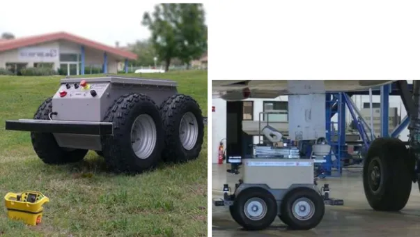
The following section will give a brief introduction of the hardware of the Air-Cobot robotic platform. All electronic equipment (sensors, computing units, communication hardware, etc.) is carried by the 4MOB platform provided by Sterela, an engineering constructor which usually works for the military sector. Figure 2.1 presents this 230 kg platform and the current state of sensor integration. The name of the platform is
given by its four-wheel skid steering drive. With a maximum speed of 5 m/s4, the
platform can run for about 8 hours thanks to its lithium-ion batteries. With all the sensory however, this autonomy is reduced to 5 hours of operation. For safety reasons (the platform weights about 230 kg) the platform itself is equipped with two bumpers that are located in front and in the rear of the robot. If for some reason one of them is compressed the platform will stop all electric motors and engage its brakes until the ”emergency stop” state is canceled manually by the operator.
Further sensors that where added for the Air-Cobot mission are: • four Point Grey cameras;
• two Hokuyo laser range finders;
• one Global Positioning System (GPS) • a single Initial Measurement Unit (IMU) • one Pan-Tilt-Zoom (PTZ) camera
4
2. Navigation Strategy
(a) Robot platform, 4MOB, designed by Sterela
(b) Robot platform fully equipped during an experimental test run next to an A320
Figure 2.1.: 4MOB platform and fully integrated Air-Cobot • a highly precise Eva 3D scanner manufactured by Artec
The sensor interfacing framework that is used throughout the project is the Robot Operating System, ROS (Hydro), on a Linux (12.04) machine. A second industrial computer that runs Microsoft Windows is mainly used for the interface with all the None-Destructive Testing algortihms while the Linux machine hosts all supervisor and navigation functionalities.
Figure 2.2 shows the remote for the 4MOB Sterela platform and the possible tablet interaction with Air-Cobot. Currently this interaction is still quite basic (Go to, Switch to). However, in the future, the pilot is supposed to monitor the status of the pre-flight inspection through such an interface.
2.2.2. The Robot Operating System
The following paragraph will give a brief overview about the Robot Operating System (or short ROS), the middleware that was used in the Air-Cobot project. One can basically refer to this software as the foundation of the Air-Cobot projects framework. This middleware allowed for fast integration of new features. Of course a new controller is much faster developed (’rapid prototyping’) in MATLAB / MATLAB Simulink, which is why a MATLAB based simulation environment was used for exactly this reason. In Sections 2.2.7 starting on Page 56 our main prototyping environment will be presented. Since testing these controllers and features on the robot is essential to achieve the
(a) Remote used by operator when close to the platform
(b) Tablet usage
Figure 2.2.: Remote of the 4MOB platform and tablet operation of Air-Cobot goal of providing a prototype robot for autonomous aircraft inspection from scratch in the period of three years, the middleware had to be chose very early on during the project. Due to its widely accepted use in the scientific community, its portability and the amount of already available, open source software features, the team decided to utilize the Robot Operating System. Several comprehensive introductions to ROS are already available [Quigley et al., 2009], [Martinez and Fern´andez, 2013] and [O’Kane, 2014]. Furthermore, in [Crick et al., 2011] researchers try to make the framework avail-able to a broader audience by introducing Rosbridge. It is considered to be the most popular middleware in the community which does not mean that is the simplest, most robust, most generic, real time capable, etc., but it does mean that the support from the community is beyond example.
For this work and the Air-Cobot project ROS was chosen for the broad availability of already working hardware drivers (for cameras, robot CAN compatibility, interfaces for navigation modules) and reusable software stacks. Part of the navigation stack [Marder-Eppstein et al., 2010] of ROS was ”recycled” to provide tracking of the robots pose in the environment with dead reckoning, IMU inputs, occasionally visual odometry and occasionally highly precise localization information that was taken as ground truth. All of this implemented in a extended Kalman filter to provide sufficiently accurate pose tracking even throughout lengthy time periods. The navigation stack is just one example why ROS can be extremely helpful.
A major downside of ROS however is that providing real time computation can be difficult. Since the software is running on top of a Linux desktop system it naturally inherits all of its short comings. These are surely minor for our prototype, since sampling control inputs for the robot can still be ensured around frequencies up to 30 Hz. Even if we consider dynamic obstacles at higher speeds the robot is able to break early enough, because equipped laser range finders can sense up to 50 meters ahead of the robot. Still, especially in areas where this ’viewing distance’ is artificially shortened (corners
2. Navigation Strategy
that keep obstacles in the sensor shadow, etc.) the robots speed needs to be adjusted accordingly.
2.2.3. Perception “ exteroceptive” (cameras and lasers) and
“proprioceptive” (odometer)
As mentioned in the previous subsection, different sensors have been mounted on the Air-Cobot platform. We review them briefly, showing how the data have been treated to be useful for the other processes. We first consider the exteroceptive sensors (vision and laser range finder) before treating the proprioceptive ones.
Detection and Tracking Features of interest by vision
Several cameras have been embedded on our robot. They are positioned on top of stereo camera systems (stereo basis of 0.3 meter) at the front and at the rear of the robot. Furthermore, a Pan-Tilt-Zoom camera system which usually is used for surveillance has been integrated on the platform. We first detail their specifications before explaining the image features processing implemented on the robot.
Specifications of cameras The four cameras that are used on the stereo camera sys-tems (front and rear) are provided by PointGrey (now FLIR). All of them are of the type F L3 − F W − 14S3C − C with 1.4 mega pixels, a global shutter, a maximum resolution
of 1384 by 10325. and a 4.65 µm pixel size. Furthermore, the focal length is 6 mm and
with four cameras the maximum refresh rate that the platform can handle is 25 Hz 6.
These cameras are all connected via 1394b firewire.
The second vision sensor in use is a PTZ camera by the producer Axis. Mainly used for the None-destructive testing part of the mission this camera does not have a global shutter. A global shutter is very important for the robustness of navigation algorithms. This camera is equipped with a photo sensor that features a much higher resolution 1920 by 1080. Furthermore, the camera system itself is able to rotate about completely about its vertical axis and 180 degrees about its horizontal one.
Target detection and tracking algorithm An algorithm “Track Feature Behavior” al-lows for tracking features while the robot remains fixed. We simply compute the center of all available features currently tracked and keep this point in the center of the image plane. This algorithm is mostly used for moving the cameras into a more favorable position (e.g., for visual servoing reinitialization) during the execution of missions. In addition, the robot does not need to be kept stationary while executing this algorithm, if the module is provided with localization information from odometry, GPS or visual
5
The maximum resolution used in the project is 800 by 600 to allow for faster refresh rates
6
Here the platform is the bottleneck since the theoretical limit for the cameras at 640x480 would be 75 Hz
Detection and tracking Obstacles by laser range finders
Now we consider the second exteroceptive type of sensor mounted on our robot, the laser range finder (or short LRF). As previously mentioned, two laser range finders have been installed: one in the front and the other one in the rear. We first detail the specifications of the chosen sensor before focusing on the algorithm developed to detect static and moving obstacles.
Specifications of the Hokuyo laser range finder The obstacle detection is performed with the help of two Hokuyo UTM−30LX laser range finders (operating at wavelength of 870nm). One Hokuyo LRF is located in the front of the robot while the other one is
located at the rear. These laser range finders each have a range of 270◦ with a resolution
of 0.25◦ meaning that there are 1080 measurements sampled on the full range of the laser.
The two LRFs are mounted on pan tilt units, therefore, enabling a 3D range acquisition of data. If the aspect is not very important for obstacle detection, it appears to be very valuable for the relative localization of the robot towards the aircraft as discussed in Section 2.2.5 (Page 45). Additionally, in the future the robot will equipped with a sonar belt, thus, eradicating blind spots due to laser placement and robot geometry. Contrary to current sensor sets for semi-autonomous vehicles such as the Tesla Model S, recent models of the Mercedes-Benz S-Class, etc, the blind spot on the Air-Cobot is extremely small.
Currently however, the two laser range finder solely provide the raw obstacle detection. The raw data is sent at a much higher interval (50Hz) than it is actually processed (20Hz). Processing this data is done in several steps. First, a cleaning operation allows to remove outliers. Then, a dedicated method provides additional informations about the obstacles such as an estimate about geometry and center of gravity or furthermore linear and angular speeds. The following section will give a more detailed insight into this process.
Obstacles detection and tracking Algorithm The following section details how ob-stacles are detected and tracked. Figure 2.3 and pseudo algorithm 2.1 show a brief overview about the data acquisition and the successive processing which are applied. First, the raw LRF measurements are read and filtered to remove outliers. Then, the remaining points are clustered into separate sets. Finally, a RANSAC method allows to classify the obstacles between circles and lines. Each step helps the system to refine / reduce the amount of raw data coming from the Hokuyo LRF. Finally it is possible to achieve a tracking of the most relevant objects in the scene which in turn allows object movement prediction, even if its only valid for a very short time period. This feature
2. Navigation Strategy
can be extremely helpful to perform a smooth and robust obstacle avoidance, especially in case of dynamic obstacles occlusions or when the object lies in a robot blind spot. Algorithm 2.1 Obstacle Detection Algorithm
1: Receive Hokuyo raw laser measurements
2: procedure LRF data processing ⊲ Callback function of laser
3: Clean the raw data by removing isolated points or accumulations of points that are
below a predefined threshold
4: Cluster the remaining points into separate obstacles
5: Perform a RANSAC on these separate obstacles to determine whether any of these
obstacles are either lines or circles
6: end procedure
7: Distribute information to the supervisor and obstacle avoidance
Figure 2.3.: Obstacle detection step by step
Figure 2.3 gives a step by step visualization of the concept explained in the pseudo algorithm 2.1. Each step helps the system to refine / reduce the amount of raw data coming from the Hokuyo laser range finder. Finally it is possible to achieve a tracking of the most relevant objects in the scene which in turn allows object movement prediction even if its only valid for a very short time period.
Odometry
The following section will review the different platform odometry systems. The basic odometry at hand has been progressively improved by adding more and more advanced techniques whose results have been fused (see the localization process for more details).
2. Navigation Strategy
Wheel Odometry Now, we focus on the first proprioceptive sensor: the wheel odome-try. It has the advantage to be very simple and fast. The Air-Cobot platform is equipped with wheel tick sensors. Through simple geometric relationships (wheel diameter, axle distance, etc.), the wheel movements can be translated into a full body motion of the robot in the world-coordinate-system.
The platform linear and angular velocities νrobot and ωrobot can be easily deduced from
the four left and right wheels velocities, as shown by equations (2.1) and (2.2):
νrobot = vlinr+ vlinl 2 (2.1) ωrobot = vlinr − vlinl 2 × dtrack−width (2.2)
where vlinr represents the average between front right and rear right wheels and vlinl
accordingly for the left side. These velocities (νrobot and ωrobot) are expressed in the
points defined by an imaginary axle exactly in the middle of front and rear driving axle. Inertial Measurement Unit (IMU) Odometry Our robot is also equipped with an Inertial Measurement Unit (IMU). It consists of three accelerometers that register the linear acceleration around x, y, z and three gyroscopes which measure the angular veloc-ities around these last axes. This sensor can help out in areas where the wheel odometry fails (see section 2.2.5).
2.2.4. Modeling: both topological and metric maps
Now, we present the modeling process. As previously mentioned, three maps are avail-able, a topological one and two metric ones. The two metric maps differ in their coor-dinate origin. The first one is centered in the robot last reset point and the second in the aircraft to be inspected. Let us first consider the topological map:
Topological map
As explained earlier, the topological map is made of the sequence of checkpoints to be reached. This list is known before the navigation begins and is derived from an existent checking schedule for airport staff or aircraft crew. The map has been optimized and the number of checkpoints reduced, as the robot is enhanced with sensors which allow to
inspect several items at a time7. Figure 2.4 shows an example of such a map. As stated
in the introduction, the main advantage of the topological map that it is in general more robust than a metric map, when it comes to localization.
The checkpoints are expressed both in terms of visual features and of relative positions with respect to the aircraft plane. This is possible because a 3D model of the aircraft is
7
This is possible if the checkpoint is carefully chosen.
✁ ✂ ✄ ☎ ✆ ✝ ✞ ✟ ✠ ✄✄ ✄☎ ✄✂ ✄✝ ✄✆ ✄✁ ✄
Figure 2.4.: Example of a navigation plan around the aircraft
Metric map
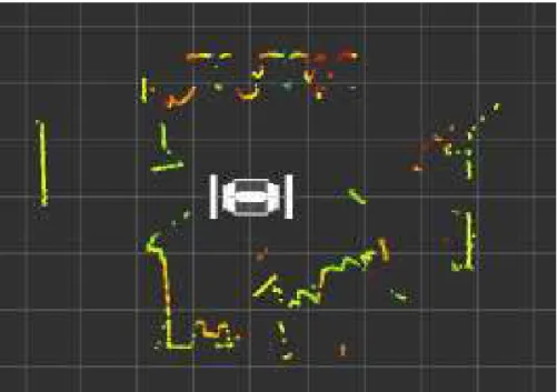
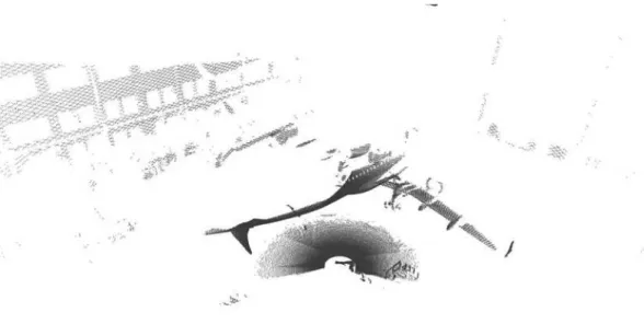
As mentioned earlier, in addition to the topological map, two metric maps are available. The first one is centered on the robot last reset point and the second one on the aircraft to be inspected. They are generated from the data provided by the laser range finder located at the front and at the rear of the robot (e.g.: SLAM). Through knowledge about the detected objects position, it is possible to fuse the incoming data onto a map. Map building is performed with a software from the ROS-Nav-Stack. Figure 2.5 shows an example of such a map (top view). It has been generated by the embedded Hokuyo LRF. In the map center, one can see the robot represented with a simplified geometric
form. The squares in this example have the size of 1m2 and all dots are instances in
which the laser rays have been reflected by the environment. Each color provides an indication of the materials emission coefficient. This map can help the user to put the data into perspective.
![Figure 1.1.: Extract of article [Frey and Osborne, 2013]; Likelihood of computerization of several jobs](https://thumb-eu.123doks.com/thumbv2/123doknet/14536976.724217/23.892.316.568.151.544/figure-extract-article-frey-osborne-likelihood-computerization-jobs.webp)