Three essays on housing markets and housing policies

(1)

HAL Id: tel-02097496

https://tel.archives-ouvertes.fr/tel-02097496

Submitted on 12 Apr 2019

HAL is a multi-disciplinary open access archive for the deposit and dissemination of sci-entific research documents, whether they are pub-lished or not. The documents may come from teaching and research institutions in France or abroad, or from public or private research centers.

L’archive ouverte pluridisciplinaire HAL, est destinée au dépôt et à la diffusion de documents scientifiques de niveau recherche, publiés ou non, émanant des établissements d’enseignement et de recherche français ou étrangers, des laboratoires publics ou privés.

Three essays on housing markets and housing policies

Zhejin Zhao

To cite this version:

Zhejin Zhao. Three essays on housing markets and housing policies. Economics and Finance. Univer-sité de Lyon, 2018. English. �NNT : 2018LYSES033�. �tel-02097496�

(2)

UNIVERSITE´ DE LYON- ECOLEDOCTORALE SCIENCESECONOMIQUES ET GESTION NNO486 UNIVERSIT E ´ JEAN MONNET

Groupe d’Analyse et de Th´eorie Economique Th`ese de Doctorat (NR) de Sciences Economiques

Pr´esent´ee et soutenue publiquement par

Zhejin ZHAO

20 septembre 2018

en vue de l’obtention du grade de docteur de l’Université de Lyon délivré par l’Université Jean Monnet

T

HREE ESSAYS ON HOUSING MARKETS AND HOUSING POLICIES

Jury :

Florence Goffette-Nagot - Directrice de recherche CNRS, Université de Lyon, Directrice de thèse Frédéric Jouneau-Sion - Professeur, Université de Lyon 2, Examinateur

Miren Lafourcade - Professeur, Université Paris-Sud / Paris-Saclay, Examinatrice Maëlys de la Rupelle - Maˆıtre de conférences, Université de Cergy-Pontoise, Examinatrice

Benoˆıt Schmutz - Maˆıtre de conf´erences HDR, Ecole Polytechnique et ENSAE, Rapporteur

External reviewer :

Chunbing Xing - Professeur, Beijing Normal University (Chine), Rapporteur externe

(3)

(4)

University of Saint- ´Etienne is not going to give any approbation or disapprobation about the thoughts expressed in this dissertation. They are only the author’s ones and need to be considered such as.

(5)

(6)

Acknowledgements

Finishing my PhD thesis is a milestone in my life. I am so lucky to have this great opportunity to pursuit a PhD. I would like to thank all those who have supported me in the completion of this thesis.

First and foremost, I would like to express my deepest gratitude to my advisor Florence Goffette-Nagot, for whom I am indebted the most during the PhD period. Before meeting her, I knew nothing about urban economics. It was she that introduced me into the field, which is very cool and powerful to explain many issues in urban areas. She has guided me throughout the past five years with so much care, dedication, patience and impressive intelligence, until the completion of my PhD thesis. During the course of this PhD, I not only got academic training from her, but also learned various traits of having a great personality. I have been impressed by her rigorous thinking, hard-working, academic enthusiasm, patience and responsibility. To be honest, she has changed me a lot. I am very appreciated to have such a kind and conscientious supervisor! I also thank her for her kind co-operation as a coauthor in the writing of the first chapter in this PhD thesis. I look forward to continue working with her after my thesis defense.

I would also like to express my gratitude to Russell Davidson for inviting me to visit the department of Economics, McGill University from November 2014 to May 2015. I learned quite a lot from his econometrics courses. I am also indebted to Saraswata Chaudhuri, Rohan Dutta and Victoria Zinde-Walsh for their permission to let me take part in their courses at McGill University. I wish to extend my special appreciation to Saraswata Chaudhuri who gave me helpful suggestions and encourage-ment for my first chapter. Many thanks to the PhD students at McGill including Tianyu He, Yang Li and Qi Xu who gave me a lot of support to help me adapt to the environment at McGill.

I would also like to thank the committee members. I am particularly grateful to Benoˆıt Schmutz and Chunbing Xing for accepting to be reviewers on this thesis and to Frédéric Jouneau-Sion, Miren Lafourcade and Maëlys de la Rupelle for being the part of the jury. In addition, I want to thank Sylvie Démurger and Maëlys de la Rupelle as the committee members when I finished the fourth year of my PhD.

(7)

This PhD thesis would never haven been completed without the support of several institutions. I acknowledge University of Saint- ´Etienne and the Ministry of Higher Education, Research and Inno-vation of France for awarding me a thesis grant for my study in France. I am also grateful to the Region of Rh ˆone-Alpes for awarding me the Explo’ra scholarship to support me to stay at McGill University in Canada. Last but not the least, I highly appreciate the generosity of the GATE Lyon-Saint-Etienne (GATE LSE) for supporting me to attend lots of academic conferences, workshops and summer schools, which is vital to my academic career.

I would like to thank Sonia Paty, the director of GATE, and Marie-Claire Villeval, the previous direc-tor of GATE, for providing PhD students with perfect working conditions and research environment. In the past five years, I have greatly benefited from faculties, fellow PhD colleagues and visiting scholars at GATE. First, I would like to say a big thanks to Sylvie Démurger who had introduced Florence Goffette-Nagot to me when I just arrived at Lyon as a master student in 2012. During the process of thesis writing, she gave me a lot of useful suggestions. She is always nice and helpful. Sec-ond, I have to mention Pierre-Philippe Combes, who always replied my emails promptly and helped me improve my thesis quality. Although he is quite busy, he spent a lot of time on listening to my presentation and taught me how to think about questions from the perspective of economic theory. I learned a lot from him. Third, I have to mention Samia Badji, Jonathan Goupille-Lebret, Tidiane Ly, Benjamin Monnery and Yohann Trouvé. I enjoyed from discussing with them and got valuable feedbacks on thesis. Fourth, a special thanks to Clément Gorin, who taught me a lot of programming skills, especially in R. In addition, I also wish to express my gratitude to the following persons for their help and advices: Sylvain Chareyron, Damien Cubizol, Frédéric Jouneau-Sion, Yann Kossi, Carl Lin, Philippe Pololmé, and Hui Xu.

I am thankful to administrative staff at GATE. I have to mention Nelly Wirth who always sends me a lot of papers closely related to my thesis, which is quite useful for my thesis writing. Many thanks to Ta¨ı Tao, Aude Chapelon, Yamina Mansouri and B´eatrice Montbroussous for their supports.

I would also like to thank Jan Rouwenda for helpful suggestions on my second chapter when I partic-ipated the summer school in Copenhagen in August 2017. For many helpful comments, I thank the seminar, workshop or conference participants at GATE, the Regional Studies Association Early Ca-reer Conference 2015, the 8th Annual SEBA-GATE Workshop 2017, the 11th International Conference on the Chinese Economy 2017, AFSE 2018, and the RUSE workshop 2018.

Thanks to the BNU-GATE master exchange program. Without it, I would not have the chance to come to France. In April 2012, when I studied in the library in Beijing Normal University (BNU), professor Chengyu Yang asked me to come to his office. He told me that there was an exchange

(8)

program between BNU and GATE LSE. He strongly encouraged me to applying for it because he visited GATE before and had a good impression on it. Fortunately, I was admitted into the GAEXA master program. Here, I would like to thank especially Chengyu Yang.

As my thesis consists of three empirical chapters, the dataset are very important and indispensable for thesis writing. I thank Lo¨ıc Bonneval for sharing the historical data on Lyon and co-working with me in the first chapter. I thank Jianwei Xu for sharing the Chinese Urban Household Survey data, which is the main dataset in the second chapter. I thank Shi Li for sharing the 2000 and 2005 micro census data in China, which is used in the third chapter. I thank Zhilong Li from National Bureau of Statistics of China for helping calculating variable values at the city level in 2010 for the third chapter. I thank Liang Wenquan and Lu Ming for providing land transaction data, although finally I did not use this dataset in the third chapter. Special thanks to Miao Tong for calculating topographic data at the city level using GIS software, which is used to construct one of instrumental variables in the third chapter. Without their contributions, it would not be possible for me to finish the chapters.

I would also like to thank my friends in Lyon who have diversified my life and made me less stressful: Bin Bao, Zhixin Dai, Xinrong Huang, Jinping Li, Tiruo Liu, Lei Mao, Yifan Yang, Jin WU, Meng Wu, Han Zhou, Mengbing Zhu, Min Zhu and Guang Zhu etc. I also have a personal friendship with Tidiana Ly. We had dinner in restaurants regularly.

A big thanks for the support from many friends and researchers in China and Canada: Weiguang Deng, Chuanchuan Hou, Hongquan Lian, Dongran Sun, Dongdong Tian, Tianyu Wang, Shafu Zhang, Yifan Zhang etc. In particular, I am indebted much to Chuanyong Zhang for his trust, encourage-ment, and his dedication to help me improve my thesis quality.

I would like to thank Dongchen Zheng, the love of my life. Thanks for all that she has done for my family. When I encountered difficulties in research, she always encouraged me and tried to make me continue to move on. In order to make me focus on thesis writing, she did a lot of housework. I am so lucky to have a wife like this. In October 2017, my daughter, Kuoyu Zhao, was born in Lyon. She has been bringing me numberless happiness and huge motivation to pursuit my academic dream. I hope to be an good example for my dear daughter. In addition, I am always indebted for support from my family members, including my mother, my young sister, my parents-in-law and other relatives.

Finally, this thesis is dedicated to the memory of my father, Wusuo Zhao, who passed away in July 2013, four months before I started my PhD.

(9)

(10)

List of Tables

2.1 Summary statistics during the period 1890-1968 . . . 20

2.2 The regression results between two adjacent periods . . . 23

2.3 Dynamic regression outputs in three adjacent periods . . . 26

2.4 The effects of rent control on rents during the period 1890-1930 . . . 27

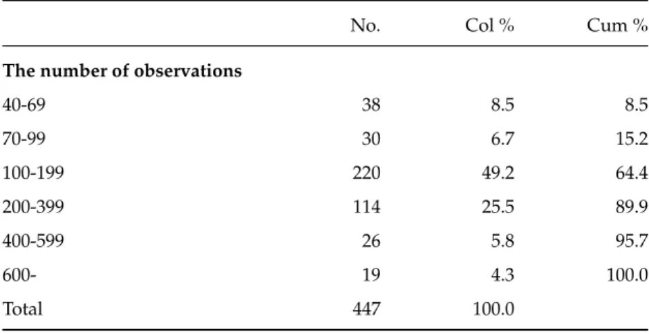
3.1 Distribution of the number of observations at the city level in the sample . . . 39

3.2 Summary of annual rents by tenure . . . 40

3.3 Characteristics of housing, household head and households in 2007 and 2009 . . . 42

3.4 The first hedonic regression results with homogeneous restrictions, 2007-2009 . . . 46

3.5 Selected results of second-stage hedonic regression for computed MWTP of housing characteristics, 2007-2009 . . . 47

3.6 Descriptive statistics in the UHS data, 2007-2009 . . . 56

3.7 The first hedonic regression results, 2007-2009 . . . 58

4.1 Summary statistics for variables in levels . . . 71

4.2 OLS regression results in 2000 and 2010 . . . 74

(15)

4.4 First stage regression results in 2010 . . . 76

4.5 IV regressions after dropping four first-tier cities . . . 77

A1 Distribution of the number of observations at the prefecture-level city in the micro censuses data . . . 79

A2 Counties or county-level cities which upgraded to urban districts between 2000 and 2010 80

A3 Source of data used in this chapter . . . 81

(16)

List of Figures

2.1 Ceilings on relative rent increases . . . 13

2.2 The number of flats in each year during the period 1890-1968, Lyon . . . 15

2.3 The number of tenants by categories in each year during the period 1890-1968, Lyon . 15

2.4 Duration and control status of flats during the period 1890-1968 . . . 17

2.5 Average rents of flats in Lyon, 1890-1968 . . . 18

3.1 The partial and global WTP for selected characteristics of houses along with age . . . 51

3.2 The WTP for a constant-quality house of a representative household by age group . . 53

4.1 Correlations between residuals and log population by year . . . 72

4.2 Correlations among housing prices, population and SIR . . . 72

(17)

(18)

Chapter 1

General Introduction

The housing market is always a hot topic for people who live in urban areas and it attracts a lot of interest in both academia and industry. In this dissertation, I investigate three aspects of the housing market and housing policies. In the first essay, I am concerned about the role of government inter-vention in housing markets. Specifically, I examine the effects of a rent control policy on rents using historical panel data from Lyon, France. In the second essay, I am interested in factors which affect the housing markets. I use micro-level data to investigate how housing demand varies with age in urban China. In addition, I also want to know the impacts of rising housing costs on the local economy. In the third essay, therefore I use census data at the county level to examine the effects of housing costs on the skill intensity ratio across Chinese cities. The research findings about housing markets and housing policies not only explain the phenomenon that happened in France and China, but also apply to other countries and make contributions to the existing literature on housing economics.

The first essay, entitled ”The impact of rent control: investigations on historical data in the city of Lyon”, reexamines the conventional claims made by economists and policymakers concerning the effects of rent control on rents. As an important form of government intervention, rent control policy has a long history in European countries and the U.S. Generally speaking, there are two types of rent control policies. Rents can be always regulated, regardless of whether the tenant is new. This type of rent control is referred to as the first generation or old-style rent control. The second generation of rent regulation is less tight. Rents are controlled for only when tenants stay in the dwelling.

Theoretically, rent control has ambiguous effects on rents. Basu and Emerson (2003) demonstrate that monopolistic landlords have the motivation to hold rents down to attract a better ‘quality’ tenant if rents are controlled for. However, Nagy (1997) argues that, under the regulation of the second-generation rent control policy, landlords could set a higher price for new tenants at the beginning in

(19)

order to make up for a loss because of a rent freeze in later periods. Early (2000) and Diamond et al. (2018) think that, in the long run, rent control might decrease housing supply, and cause rents to rise even in the controlled sector.

Therefore, it is necessary to examine the effects of rent control on rents. In the literature, a lot of papers have addressed this issue using evidence from cities in the U.S. (See Gyourko and Linneman (1989), Nagy (1997), Sims (2007), Autor et al. (2014) and Diamond et al. (2018)) However, few papers use data from European countries to evaluate the impacts of rent control on rents. Mense et al. (2017) find that the rent cap implemented in Germany decreased rents and housing prices in the regulated sector, but increased them in the unregulated sector. The first essay of this thesis uses unique panel data at the flat level from a property manager’s accounting books in Lyon during the period 1890-1968. The estimation results show that rents decrease when flats are controlled for. The first generation rent control policy have larger negative impacts on rents than the second generation.

The housing market is influenced by many factors. The demand-side factors, such as monetary policy, the state of the economy, household income and demographic structure, and housing supply, influence housing prices. Mankiw and Weil (1989) suggest that population aging can cause housing prices to decline in the long run. Ortalo-Magne and Rady (2006) show that the ability of young households to afford the downpayment on their first house and their income are powerful drivers of the housing market. Taylor (2007) claims that excessively expansionary monetary policy during the period from 2002 to 2005 is a cause of a bubble in the housing market in the U.S. Ferreira and Gyourko (2011) show that income of prospective buyers is a fundamental factor of the housing boom across U.S. metropolitan areas from 1993 to 2009. Switching to supply-side factors, Glaeser et al. (2005) and Saiz (2010) show that inelastic housing supply caused by physical and regulatory constraints have positive impacts on housing price appreciation across American cities since 1970s. Liang et al. (2016) argue that the misallocation of construction land supply between coastal and inland regions cause housing prices to rise faster in coastal cities than those in inland cities in China. Dong (2016) uses a sample of 35 major cities in China from 2003 to 2012 to find that both natural and man-made constraints imposed on housing supply are positively correlated to housing price appreciation.

With rising housing demand and limited housing supply, housing prices and rents will unavoidably rise. This is what happened in China in recent years. The high and rising prices in Chinese housing markets have generated global interest. Real prices increased by 160% between 1997 and 2011 ac-cording to China Statistics Yearbook. People want to know which factors cause such fast increase and whether the housing price will continue to rise in the future. Considering the difficulty of measuring housing supply at the city level in China, I focus on fundamental factors of housing demand.

(20)

Specif-ically, the second essay of this thesis studies how housing demand, quantity and quality of housing services, varies with age at the household level using micro-level data from urban China during the period 2007-2009. Since Mankiw and Weil (1989) explored the effects of demographic structure on housing markets and concluded that the housing demand in the U.S. will decline with population aging in the next 20 years, this question has attracted a lot of attention. However, previous literature does not isolate completely the role of demographic changes and other socio-demographic factors which may affect housing markets.

In the second essay of this thesis, I use the two-stage hedonic price model to investigate the corre-lation between housing demand and age. The data I use is the Chinese Urban Household Survey (UHS) from 2007 to 2009. This survey is conducted by the National Bureau of Statistics of China (NBSC). The NBSC uses a stratified random sampling to select cities and towns as surveyed regions in the UHS. What I could get access to is the subsample in 16 of 31 provinces from 2007 to 2009, which represents 65% of China’s population(NBS, 2013). The UHS survey contains detailed characteristics of housing such as space floor area, housing age, rents and a lot of facilities, and that of households such as age, gender, marital status, income and educational attainment.

Specifically, I calculate the age specific implicit willingness-to-pay for a representative housing in the sample. In the first stage, I regress housing expenditures on all characteristics of a house to get the implicit price for each hedonic characteristic. In the second stage, I regress the calculated implicit prices on all characteristics of housing and socio-demographic characteristics of households as well as year dummies. Finally, I get the partial relationship between housing demand and age, because all socio-demographic characteristics except age have been controlled for. I can get the global relation-ships between housing demand and age if I do not control for any socio-demographic characteristics of households except age in the second stage, which means that the housing demand of households is allowed to change with characteristics of households. Considering that some socio-demographic characteristics such as marital status change with age naturally, and some characteristics such as ed-ucational attainment are constant over the life-cycle of households, I control for socio-demographic characteristics which change with age in the second stage, and then I got the third relationship, i.e. composite relationship between housing demand and age.

The partial and composite curves relating housing demand to age depict flat or slightly negative trends when people are older than 65. However, the global curve between housing demand and age shows that housing demand decreases with age. The overall results suggest that educational attainment largely drives the relationship between housing demand and age, while age does not have negative impacts for the housing demand as long as educational attainment is controlled for.

(21)

In the context of China’s higher education expansion and rising urbanization rate, this second essay predicts that aggregate housing demand will not drop with population aging.

Because the UHS used in the second essay covers only three years, I cannot disentangle cohort effects from age effects. Instead, I have to assume that cohorts have similar preferences for housing. I have to test the validity of this implicit assumption if more datasets are available in the future. In addition, the UHS mainly focuses on households with local hukou, and migrants are under-represented. Hence the computed housing demand of a representative household might be overestimated.

After analyzing the determinants of housing prices, it is natural to think about consequences of a booming housing market. Considering that housing cost is one of the most important components of living cost across cities, what is the impact of housing costs on spatial dispersion of the labor force? The third essay applies the Rosen-Roback model and its extensions to investigate how housing costs affect the skill intensity ratio (SIR) of labor force across cities in China. The SIR is defined as the the ratio of college graduates to non-college graduates among adults aged 25 years old or above. Rosen (1979) creates a model of inter-city wage differences and makes a hypothesis that migration across metropolitan areas should cause equality of indirect utility. In the original model, Rosen (1979) as-sumes that all workers are homogeneous. The model suggests that wage differentials across cities arise due to relative price or amenity differentials associated with inter-city different characteristics including city size or growth rate. Kim et al. (2009) develop the models above by allowing for het-erogeneity in housing preferences and human capital for workers, and they demonstrate that living costs of high- and low-skilled workers have different change rates, which is associated with changes of wage differentials between high- and low- skilled workers within one city.

Following their model, I use China’s 2000 and 2010 censuses and corresponding data at the city level to test the model and show that rising average housing prices increase the ratio of skilled to unskilled workers in 2010, when workers’ mobility was relaxed. However, effects of average housing prices on the SIR is only significant at the 10% level in 2000, when the hukou regulation was tight. As housing prices are endogenous, I use elasticities of housing supply based on land slope and historical housing prices as instruments of average housing prices. I also find that housing prices have significant positive effects on shares of high-skilled workers, but insignificant negative effects on shares of low-skilled workers in 2010 after taking into account the endogeneity issue. This essay confirms the validity of Rosen-Roback model.

This essay is closely related to the research by Broxterman and Yezer (2015), which examine the role of housing cost in determining the SIR across cities using data from the U.S. decennial census over the period 1970-2000. Unlike them, I use a novel instrument for housing prices and focus on the rapidly

(22)

rising real estate market using newly available data in China. Because the census survey does not have information on wages, I cannot estimate the effects of housing costs on the wage differences between high-skilled and low-skilled workers using a direct way.

To summarize, separately the three essays represent important additions to their respective litera-ture. Together they help to understand the role of government intervention in housing markets, the deterministic factor of housing markets, and impacts of housing markets on the labor market.

(23)

(24)

Chapter 2

The impact of rent control: investigations

on historical data in the city of Lyon

1

2.1 Abstract

This chapter reexamines the conventional claims made by economists and policymakers concerning the effect of rent control. We consider the impact of rent control on rents using panel data in Lyon over a 78-years period. Our study is a comprehensive empirical study of different rent control forms using multiple regressions with fixed effects as the main form of analysis. We find that the causal effect between rents and rent control is significantly negative. Furthermore, more restrictive rent control policies cap rents more tightly.

2.2 Introduction

A new housing rent freeze law began to take effect in France in September 2012, which was presented by French Housing Minister C´ecile Duflot in order to reduce housing rent increasing trend. This was the first step towards a new system of rent controls proposed by President Franc¸ois Hollande. As rents rise sharply in France, this decree will prevent any increase when a landlord lets a property for the first time or relets it. On the one hand, this regulation is able to cap increases in rents immediately, on the other hand, it discourages investments in the property sector, so that housing supply might be insufficient compared with housing demand in the long run. In this case, the real rents might be higher than if the rent control policy had never been implemented. This policy also has some impacts

(25)

on maintenance expenditures of rental housing units. Landlords spend less on housing maintenance due to rent control, because they are not able to get the same prices as those in the uncontrolled markets. Their rational choice is therefore to decrease their inputs. However, Moon and Stotsky (1993) show that tenants have more incentives to invest in maintenance of their dwelling in order to compensate more or less under rent controls. Could the regulation significantly decrease rents? What are its impacts on maintenance costs? This paper attempts to reexamine the effect of rent control in order to answers these two questions.

Our study tests the effects of rent control on rents using historical data in the city of Lyon over a 78-years period. During the period 1914-1968, the first and the second generation rent control policies were implemented alternatively in Lyon. We find that both forms of regulation can make rents fall in most cases, and the stricter policy has larger effects on rents.

There are some important caveats to our results. First, due to the availability of data, we cannot obtain one third buildings’ quality information, so that we have to drop other available buildings’ quality information in order to use to the whole sample, which means we do not control all variables affecting rents and maintenance costs. Another limitation is that we only have data about maintenance costs at the building level instead of the flat level. We assume every flat’s maintenance cost is decided according to its share of all floor area in the same building.

The reminder of this chapter is organized as follows. The next section presents the literature review. Section 3 describes the rent control history in Lyon and the dataset used. Section 4 introduces the methodology we use in order to process the data. Section 5 reports the results. Section 6 concludes.

2.3 Related Literature

Regulatory intervention in housing markets is broad and deep. Housing markets are governed by planning processes, zoning regulations, land use regulations, financial regulations and numerous other regulations (Turner and Malpezzi, 2003), among which rent control is the most important reg-ulation historically (Gyourko, 2009) .

There are two types of rent control. The rents can be controlled even when the tenant changes. Conventionally, it is referred to as the first generation rent control. This is the type of control that was implemented in Lyon during the 1930-1948 period. This form of rent control was a restricted freeze on nominal rents, that is, the government set absolute ceilings on rents. So it is very strict. Conversely, rent control can work unless the tenant changes, which means rents are regulated only

(26)

within a tenancy. We often call this kind of rent control the second generation rent control policy.

Several studies indicate that rent control can reduce rents in the controlled sector. Gyourko and Linneman (1989) regard the constrained rents as a subsidy to the tenant. They find a mean annual subsidy in a rent controlled unit of 27.2% of annual income by analyzing New York’s rent control system in 1968. Raess and von Ungern-Sternberg (2002) show that the second generation rent control can limit the owners’ abilities to increase rents for a certain contract and leads to lower equilibrium rents, when price discrimination is caused by the existence of product heterogeneity, search costs and switching costs.

Basu and Emerson (2003) also study the effect of the second generation rent control on rents. They think its impact is similar to the first generation rent control policy. Because of inflation and infor-mation asymmetries, landlords prefer short-staying tenants to long-staying tenants, but they cannot distinguish which type the tenants are. The long-staying tenants have the incentive to conceal this in-formation to prospective landlords. Considering this point, monopolistic landlords hold price down to attract a better ‘quality’ tenant (i.e. one who will stay short). Therefore, the second generation rent control can reduce rental levels in a way that mimics old-styled rent control policy. Sims (2007) estimates the effect of rent control in Massachusetts on the rent of renter-occupied apartments. He got the similar conclusion that rent control reduces rents substantially.

However, some studies question whether rent control policy lowers rents in the controlled sector. Nagy (1997) argues that landlords can set a higher price than the rents in an uncontrolled market in order to compensate the impact of the second generation rent control, because the rents will have to remain unchanged until the tenants change. However, as the time goes, the rents paid by tenants in the controlled sector will increase. Therefore, these regulations may change nothing except for altering the timing of rent increases. Nagy uses data from New York City to test for this hypothesis. The author finds that new tenants paid higher rents in controlled sector in New York City compared with those who occupied similar apartments in an uncontrolled sector in 1981. However, tenants in the same controlled sector paid less in 1987.

Some studies even argue that rent control results in higher rents in the controlled sector. Early (2000) shows that the likely long-run effect of rent control is to make the supply decrease and the cost rise, so in the long-run, rents may be higher even in the controlled market due to rent control. He uses the data from New York City in 1996 to test this hypothesis. The results suggest that tenants lost 44 dollars per month for households in rent stabilized apartments and 4 dollars per month for households in more strictly rent controlled housing. The tenants would have been better off in the controlled sector if rent control had never been implemented in New York City. Heffley (1998) also

(27)

argues that tenants may benefit from the abolishment of the rent control policy if landlords and tenants can change their economic and location decisions. Diamond et al. (2018) show that the rent control in San Francisco increased the probability of renters staying by 20%, reduced the supply of rental housing by 15%, and led to average rent increase by 5/1%. Finally, they concluded that the rent control policy caused a substantial welfare loss.

Rent control also has an impact on the rents in the uncontrolled sector. If rent control reduces the supply of housing, this will lead to a shortage in the whole housing market. Therefore, the rents will be higher in the uncontrolled markets, too. Tenants have to pay more due to the spillover effect of rent control. This is one of the main arguments against a rent control policy. Fallis and Smith (1984) use the data of Los Angeles, California during 1969-1978 to test the effect of rent control. They find that rent control effectively raised rents in the uncontrolled segments of the markets. Early (2000) draws the conclusion that the fraction of rental units under rent control is positively correlated with the pricing of rental housing in the uncontrolled sector by testing the data of New York City in 1996. Caudill (1993) estimates the effect of New York City’s rent controls in 1968 by using both the ordinary least squares regression and frontier method. He finds that rents in the free sector would be lower by 22%-25% if control did not exist. Some economists also draw the same conclusion that rent control leads to higher rents in the uncontrolled sector (Early and Phelps, 1999; Navarro, 1985; Ho, 1992). Autor et al. (2014) find that the unanticipated elimination of rent control in Cambridge, Massachusetts, in 1995 raised housing values of both decontrolled and never-controlled residential properties.

However, the conclusion of effects of rent control on housing markets is still controversial. Consider-ing general equilibrium effects, Hubert (1993) argues that rent control policy might decrease rents in the uncontrolled housing markets because of spillover effects. Rent control acts like a subsidy, which makes housing’s demand excess in the controlled sector, so that the housing units’ allocation is like a rationing system, which makes tenants reduce their housing consumption. Consequently, the de-mand also decreases in the uncontrolled sector, so rents might decrease. Heffley (1998) gets a similar conclusion using a spatial equilibrium model of rent control: when rent control is imposed, the rent does not rise in the uncontrolled sector. Although this result depends on the model specification and parameter values, it indicates that the external effect of rent control might be complicated when ten-ants can change economic and location decisions. Sims (2007) shows that rent control usually reduce maintenance levels. So uncontrolled rental housing located nearby will decrease in value due to the potential negative spillover effects. In this case, the rent might decrease in the uncontrolled sector.

(28)

Rent control can reduce the supply of rental housing. They examine the effect of rent control on prices of uncontrolled housing markets by using 1984 to 1986 data from the American Housing Survey, and find that the price in the uncontrolled sector increased since the introduction of rent control. However, these effects decline through time and may disappear after several years.

There are also some debates about the effect of rent control on housing maintenance. Many economists think that landlords allow maintenance expenditures to fall because of the effect of rent control (Navarro, 1985; Albon and Stafford, 1990; Ault and Saba, 1990; Ho, 1992). Since the rent is con-trolled, the demand for housing excesses the supply. Landlords can make the value of housing fall in order to maximize their profits by decreasing their inputs in maintenance. Gyourko and Linneman (1989) find that a negative relationship between rent control and maintenance do exist. They draw this conclusion by using the data of New York City in 1968. They find that the impacts of rent control are lower in smaller and newer buildings. If the buildings are under ten years old, the impacts dis-appear. The biggest impacts happen in Manhattan, while the smallest happen in Queens. Under the second generation rent control, rents are controlled unless tenants change. Glaeser (2002) argues that even the second generation rent control gives strong incentives to landlords to keep housing units, the maintenance still is reduced and low quality apartments are created. Arnott and Shevyakhova (2014) argue landlords have incentives to prettify the housing only before the new tenants come in order to attract them, but few incentives to maintain the housing units well during the fixed-duration tenancy. Therefore, the second generation control leads to a decrease in maintenance.

However, Olsen (1988) thinks that the relationship between rent control and maintenance is theoreti-cally ambiguous. Because “rent control ordinances that increase the ceiling rent on an apartment generously when it is upgraded and decrease it severely when it is allowed to deteriorate will lead to greater landlord main-tenance of the unit.”, tenants have incentives to spruce up the housing due to the income effect of rent control. But, the tenants may move before receiving all benefits of maintenance activity. So they are not able to get an unambiguous conclusion about the effect of rent control on maintenance. But Mengle (1985) argues that such rent control ordinances cannot prevent the problems. It is not easy for tenants and administrative agencies to observe the real dynamic maintenance costs change. Some sanctions against landlords who reduce maintenance expenditures do not work sometimes. As Mengle (1985) illustrated, Sims (2007) thinks that rent control does reduce the maintenance in the controlled units although it does not lead to big maintenance failures because the contract about maintenance level can not be complete. For example, the tenant can ask the landlord to repair if water and heat fail, but not for cracked paint.

(29)

tenants in fixed long-term duration have more incentives to engage in self-maintenance in order to compensate more or less. They find little evidence that the first generation rent control causes hous-ing quality changes by ushous-ing data from New York City in the 1970s and 1980s. Kutty (1996) analyzes the effect of rent control on rental maintenance by establishing a dynamic model. She concludes that only the first generation rent control can reduce maintenance unambiguously, while rent control and maintenance may be positively correlated under the second generation rent control, in which rents are decontrolled between the tenancies.

2.4 Rent control history in Lyon

In 1914, due to the burden of World War One, renters were allowed not to pay their rent for periods up to 90 days if the rent was below a ceiling of 600 FF in Lyon. Based on data used in this chapter, this means that an annual average of 45% of housing rents remained unpaid between the second semester of 1914 and the first semester of 1920. This represents about 35% of total rents. After accounting for delayed payments, the total loss of landlords amounted roughly to 20% of their income.

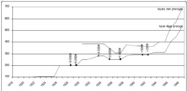
Between the World Wars I and II, a special regime was put in place, in a context where the shortage of housing and the economic situation required to protect renters. A complex system of accumulating successive rules was implemented from 1919 to 1936. It consisted mainly of a ceiling on relative rent increases, as represented on Figure 1.1.

A new law was passed in 1948, which aimed at ending the special rent regime and at increasing the return of housing properties in order to favor housing construction and maintenance. A ref-erence rent was computed based on the housing characteristics such as location, maintenance and quality. Bi-annual increases were applied in order to reach this reference rent by 1955. Continued leases ensured a capped increase of the rent. The incentive for tenants to stay in the apartment or to subcontract was high.

A first generation rent control system was implemented in Lyon during the 1930-1948 period. A second generation rent control policy was in place in Lyon during the periods 1914-1930 and 1948-1968. As we stated earlier, in the second generation rent control, rents can increase with a limited speed in order to ensure a reasonable return on investment to the landlord. Last, it is noted that some flats were out of rent control between 1928 and 1948 when the rent was higher than a certain limit as shown in Figure 2.1. For instance in 1928, rents above 9000fr were not controlled anymore. This limit changed 7 times. The last one is in 1942: rents above 250fr were not controlled anymore.

(30)

Figure 2.1: Ceilings on relative rent increases

Note: This figure is taken from Bonneval and Robert (2009). Index 100 corresponds to the rent in 1914. The “loyer l´egal prorog´e” corresponds to leases starting before 1914. Flats went out of this regime progressively when a change of ten-ant occurred or when the rent reached a ceiling. These ceilings are represented on the figure. For instance, starting on 1928, flats with a rent above 9000 FF are not controlled anymore. Starting from 1930, all rents are capped excepted those which exceed a certain ceiling.

2.5 Data and estimation method

2.5.1 Data source

This study uses data collected from a property manager’s accounting books by Bonneval and Robert (2009). The dataset gives information on flat and building characteristics for the period 1890 to 1968. Flat-level variables include whether the flat is used for housing or commercial use, whether the tenant is new or not, rent, number of rooms, floor area, storey, quality category and rent control status. Building-level variables include total rent and maintenance expenditures, location, construction type, construction period, number of floors and floor area. Monetary variables are corrected for inflation using coefficients drawn from Friggit (2002).

Our study focuses on flats used for housing. The original sample size was 32,745. We drop flats of which use is commercial or unknown, that is 8,264 observations. 1438 observations with missing in-formation for floor area or number of rooms are dropped. Flats with missing inin-formation for building characteristics are also excluded, resulting in a further reduction in the sample size by 788. The final sample consists of 258 flats and 12,749 observations. We have to correct observations with missing

(31)

information on tenant mobility in the 1948-1968 period, that is, 43 observations. In these cases, we consider there was no tenant mobility.

Part of the data is given by semester and we have to aggregate it into yearly data. If one flat is controlled at least one semester, we suppose that the flat is controlled in the whole year. We combine the variable architecture type and construction period into interactive dummy variables, because both variables are highly correlated.

2.5.2 Descriptive statistics

Figure 2.2 plots the evolution of the number of flats in each year during the 1890-1968 period. Be-tween 1890 and 1913, all observable flats were uncontrolled and the number of flats in the data in-creased from 123 to 200 at the peak of the whole period. This was followed by a reduction in the number of flats between 1914 and 1917, which means some flats disappeared from the survey, and a recovery in 1918 and 1919. The number of flats kept stable from 1920 to 1946. After that, it decreased slightly until 1968.

Starting in 1914, the rent control policy began to take effect and the number of uncontrolled flats plummeted. For example, in 1914, 169 flats were controlled, whereas only 25 flats were still uncon-trolled. Reminding that a flat was controlled during 1914-1929 if the tenant changed, we can know that most tenants were the same as those in previous years in this year. The percentage of uncon-trolled flats was 11.2% of all flats during 1914-1930. Then, the number of unconuncon-trolled flats rose rapidly until 1948. It means many flats were out of control because the rent was higher than a certain limit.

Since 1949, the rent control policy switched to the second generation rent control again and a flat was not out of control unless its tenant was new. The number of uncontrolled flats fell rapidly and then stayed low until the end of this survey. Figure 2.3 shows the number of new and same tenants by year during the period 1890-1968. We find that the share of new tenants is volatile but did not change much in the long run. When the rent control policy started in 1914, the share of new tenants decreased rapidly but then rose after few years. The same situation happened in 1949.

(32)

Figure 2.2: The number of flats in each year during the period 1890-1968, Lyon 0 50 100 150 200

The number of flats

1890

1914

1930

1949

1968

All flats Controlled flats Uncontrolled flats Source: Loic Bonneval and Francois Robert (2009)

Figure 2.3: The number of tenants by categories in each year during the period 1890-1968, Lyon

0 5 10 15 20 25 30 35 40

The percentage of new tenants

0 50 100 150 200

The number of tenants

1890 1914 1930 1949 1968

All tenants Same tenants

New tenants Percentage of new tenants Source: Loic Bonneval and Francois Robert (2009)

(33)

Figure 2.2 also shows some flats disappeared over time. Figure 2.4 shows this phenomenon more clearly. 48% of flats are present in 1890, the first year of the observation period, and 87% have been observed since at least 1914, while 3% of flats are present only after 1948. The situation is symmetric for the last year of each flat. 47% of flats were observed until 1968 and 66% until 1948, while less than 5% of flats disappeared before 1914. The average number of years a flat is present in the database is 52 years; but it should be noted that the observations are not continuous in 46% of the cases. 54% of flats are observed during the whole period, while the average number of missing years for all flats is 2.7. In addition, 13% flats miss one year and 6% flats miss two years. It should be noted that some flats reappeared after missing many years. So the panel data we use is unbalanced.

(34)

Figure 2.4: Duration and control status of flats during the period 1890-1968 Ap4 Ap120 Ap182 Ap257 Ap311 Ap373 Ap425 Ap1214 Ap1271

Flat ID

1890 1914 1930 1949 1968

Flat duration Control status change Notes: The red dot means that the control status changed

(35)

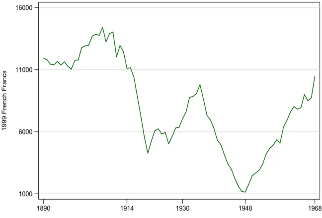
Table 2.1 presents descriptive statistics for the variables used in this study by time period and rent control status respectively. Because there was no rent control in Lyon between 1890 and 1914, we just list the variables in the uncontrolled sector. For convenience, all currency amounts are expressed in 1999 French Francs. In the periods 1914-1929 and 1930-1948, the rents in the controlled sector are on average lower than those in the uncontrolled sector. Rents experienced a sharp volatility from 1928 to 1948, as shown in Figure 2.5. In the later period 1949-1968, the rents in the controlled sector are higher than those in the uncontrolled sector. However, the characteristics of dwellings in the controlled and uncontrolled sectors change over time. In the last period 1948-1968, under the second-generation rent control, flats in the controlled sector have more rooms and are at a lower floor. However, in the second period 1914-1929, the controlled sector is further away from the center of Lyon. During the period 1930-1948, under the first generation regulation, the controlled sector is closer to the center of Lyon, but controlled flats have less rooms and are at higher floors. Both dwelling characteristics and rent control impact rents and maintenance expenditures, which means housing characteristics have to be controlled for to test the effect of rent control.

Figure 2.5: Average rents of flats in Lyon, 1890-1968

1000 6000 11000 16000 1999 French Francs 1890 1914 1930 1948 1968

Source: Loic Bonneval and Francois Robert (2009)

What we are interested in is the relationship between rent control and rents during the whole period. Before 1914, the change of average rents is not large although average rents increased from 11,011 to

(36)

15,244 French Francs between 1898 and 1907, and then fell to 12,594 French Francs in 1913 (Figure 2.5). Since 1914, with the implementation of the second generation rent control policy, the average rent dropped drastically until 1919. Then it stayed relatively stable with low volatility until 1926, and then increased again.

In 1930, the stricter rent control regulation began to take effect, while some flats were out of rent control between 1928 and 1948 when the rent was higher than a certain limit. From 1930 to 1935, rents increased rapidly. Beginning in 1936, the rental housing market in Lyon plummeted and the mean rent reached the lowest level in 1948. Rents increased again since then. We hypothesize that the rent control policy partly explains the rent trend in Lyon. We must disentangle the effect of rent control and other factors which can influence rents.

(37)

Table 2.1: Summary statistics during the period 1890-1968

1890-1913 1914-1929 1930-1948 1949-1968

Uncontrolled Controlled Uncontrolled Controlled Uncontrolled Controlled Uncontrolled

Rent 12,611 6,834 7,014 4,494 6,618 5,852 5,395

(13,222) (8,672) (9,265) (3,293) (8,964) (5,942) (5,191)

The number of rooms 3.29 3.55 3.37 2.82 4.06 3.56 3.19

(1.63) (1.82) (1.83) (1.24) (1.88) (1.91) (1.69)

Surface per room 22.97 22.04 21.49 20.52 22.72 22.01 22.49

(10.24) (9.67) (8.19) (8.33) (7.75) (8.09) (9.19)

The number of rooms

Ground floor or 1st 0.17 0.21 0.18 0.14 0.25 0.18 0.24 (0.38) (0.41) (0.38) (0.35) (0.44) (0.38) (0.43) 2nd-4th Floor 0.58 0.59 0.58 0.52 0.63 0.59 0.44 (0.49) (0.49) (0.49) (0.50) (0.48) (0.49) (0.50) 5th-6th Floor 0.25 0.20 0.24 0.34 0.12 0.23 0.32 (0.43) (0.40) (0.43) (0.47) (0.32) (0.42) (0.47)

Construction type and period

Haussmannian*1871-1914 0.39 0.41 0.36 0.37 0.45 0.42 0.38 (0.49) (0.49) (0.48) (0.48) (0.50) (0.49) (0.49) Ancient*1871-1914 0.20 0.16 0.11 0.11 0.16 0.10 0.06 (0.40) (0.36) (0.31) (0.31) (0.36) (0.30) (0.24) Haussmannian*before 1871 0.10 0.11 0.06 0.09 0.12 0.10 0.14 (0.30) (0.31) (0.24) (0.29) (0.33) (0.29) (0.35) Ancient*before 1871 0.31 0.33 0.47 0.43 0.27 0.39 0.42 (0.46) (0.47) (0.50) (0.50) (0.45) (0.49) (0.49) District District 1st 0.19 0.24 0.37 0.34 0.27 0.36 0.41 (0.39) (0.43) (0.48) (0.47) (0.44) (0.48) (0.49) District 2nd 0.42 0.37 0.30 0.34 0.32 0.28 0.30 (0.49) (0.48) (0.46) (0.48) (0.47) (0.45) (0.46) District 3rd 0.18 0.14 0.17 0.11 0.16 0.16 0.09 (0.38) (0.35) (0.37) (0.31) (0.37) (0.36) (0.29) District 5th 0.08 0.07 0.08 0.09 0.06 0.09 0.07 (0.27) (0.26) (0.26) (0.28) (0.24) (0.28) (0.25) District 6th 0.13 0.18 0.09 0.12 0.19 0.12 0.13 (0.34) (0.38) (0.28) (0.32) (0.39) (0.32) (0.33)

Distance to the city center 759 787 749 769 790 742 680

(370) (360) (335) (349) (350) (311) (305)

(38)

2.5.3 Method

Methodologically, we exploit the rent control status variation of dwellings in our database and use instrumental variables to identify the causal effect of rent control on rents at the flat level. The basic regression model in levels is the following:

Inyit = αi+ λt+ β1rc1it+ β2rc2it+ γxi+ εit (2.1)

where ln yitrepresents the logarithm of annual rent of flat i in the year t, αia flat-specific intercept, λt is a vector of year dummies, rc1ittakes value 1 for a flat controlled by the first generation (strong) rent control policy, rc2ittakes value 1 for a flat which is controlled by the second generation (moderate) rent control policy, xiare flat’s characteristics.

The flat fixed effects allow for time-constant, flat-specific factors that affect the level of rents, while the year dummies control for time variations in the level of rents.

We then write the model in first-differences, so that unobserved time-invariant factors that are spe-cific to each flat and affect the level of rents are differenced out:

∆Inyit=∆λt+ β1∆rc1it+ β2∆rc2it+ εit (2.2) In some additional specifications, we control extra variables, such as level dummies, building-specific linear time trends, different time trends for different districts within Lyon, or an interaction between the construction type (or period) and a time trend.

Throughout all models, we cluster standard errors by buildings. To address the possible existence of autocorrelation and moving averages, I also show regression results using maximum likelihood estimation of a model with ARMA. The main coefficient of interest is β. It can be interpreted as the causal effect of rent control on the flat rent.

Despite controlling for building trends and several variables at the flat level, estimation of β in re-gression model (2) by ordinary least squares (OLS) may suffer an endogeneity bias. Because rent control status is not randomly assigned to housing units, it may be correlated with some omitted variables. For example, in the period 1914-1927, the flat was controlled unless the tenant was new. Suppose that, for some reasons such as the improvement of local amenities, a flat becomes more at-tractive during this period. Consequently, the original tenant would continue to stay here or a new tenant would have to pay a higher rent. This would induce an upward bias in the OLS estimates of

(39)

β. Another problem is the reverse causation. For example, in the years 1928 and 1929, either if the

rent exceeded a certain limit or the tenant was new, the flat was out of control. If the flat rent was relatively high, the tenant would be likely to move out. This means that the magnitude of rents can change the rent control status during this period.

2.6 Main regression results

There are three types of rent control policies in Lyon in the whole period. The rent ceiling policy, which was implemented from 1928 to 1948, overlapped with other rent control measures. The gov-ernment carried out the second generation rent control policy in 1928 and 1929 as well as the first generation thereafter until 1948. In 1928 and 1929, there were only 16 observations of 12 flats which were uncontrolled by the second generation rent control policy, while there were 343 observations for 173 flats in 1928 and 1929, as well as 2,261 observations of 221 flats in 1913-1929. Therefore, we can roughly attribute the effect of rent control to the second generation rent control policy during the 1913-1929 period. From 1930 to 1948, both the first generation rent control policy and rent ceiling policy were implemented, so that we can regard the effect of rent control as their aggregated effect.

Therefore, the whole period 1890-1968 is divided into four periods: 1890-1913, 1914-1929, 1930-1948 and 1949-1968. In order to avoid very heterogeneous economic contexts, we estimate the effect of rent control between two adjacent periods one by one.

2.6.1 The OLS and FE regression results

Table 2.2 shows the main regression results between two adjacent periods. The control variables contain building type, building construction period, average surface per room, number of rooms, floor, distance to the city center and year dummies in the OLS regressions and year dummies in the FE regressions.2

(40)

Table 2.2: The regression results between two adjacent periods

Period Explanatory Variable OLS FE RE

1st generation rent control

1890-1914-1930 2nd generation rent control -0.119∗∗∗ -0.111∗∗ -0.113∗∗

(0.037) (0.028) (0.028)

Observations 6463 6463 6463

Adjusted R2 0.712 0.650 0.708

1st generation rent control -0.390∗∗∗ -0.062∗∗∗ -0.076∗∗∗

(0.053) (0.021) (0.023)

1914-1930-1948 2nd generation rent control -0.110∗∗∗ -0.090∗∗∗ -0.093∗∗∗

(0.038) (0.023) (0.023)

Adjusted R2 0.803 0.794 0.779

1st generation rent control -0.437∗∗∗ -0.187∗∗∗ -0.199∗∗∗

(0.059) (0.044) (0.045)

1930-1948-1968 2nd generation rent control -0.100∗∗∗ -0.094∗∗∗ -0.093∗∗∗

(0.039) (0.023) (0.023)

Adjusted R2 0.865 0.871 0.858

Standard errors in parentheses∗p<0.10,∗∗p<0.05,∗∗∗p<0.01

Control variables contain building type, building construction period, average surface per room, number of rooms, floor, distance to the city center and year dummies in the OLS and FE regressions.

Firstly, we get the results for the effect of rent control in 1890-1929. In the first period 1890-1914, there was no rent control. Starting from 1914, rents were controlled unless tenants changed. The estimated coefficient for our main explanatory variable is -0.151 in the basic specification and it is highly significant. The estimated coefficient in the fixed effect specification is -0.129. Based on these estimates, the coefficient of interest is around -0.140.3

Then we estimate the effect of regulation in 1914-1948. In the first period 1914-1929, rents were con-trolled unless tenants changed. After 1929, the rent control policy became stricter. Even if the tenant

3_{The average surface per room is positively correlated with rents. The higher the number of rooms, the higher the rent.}

Similarly, the higher the floor is, the lower the rent. Distance to the city center does not have any significant impact on rents.

(41)

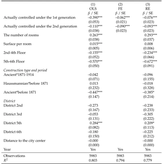
were new, rents were still controlled unless rents exceed one certain ceiling. The second column in Ta-ble 2 represents regression results in this period. We can find that the effect of the second generation rent control is still negative and significant, but it is smaller in 1914-1948 compared to the previous period. Perhaps the reason is that many flats with high rents were out of control in 1930-1948. The OLS regression shows that the first generation rent control is able to decrease rents by 46.8%. How-ever, the magnitude of the effect of the rent control policy is lower in the FE estimation, which means unobserved variables correlated to the rent control status influence rents.

Lastly, we examine the relationship between rent control and rents in 1930-1968. In the first period 1930-1948, rents were controlled even after a change of tenant. After 1948, a new rent control law was passed. If when tenant changes, the rent is not controlled anymore. In this period, the FE regression results show that the effect of the first generation rent control policy is twice larger in magnitude compared to the second generation rent control policy. The characteristics of housing units have similar influence as in the previous periods.

In sum, both rent control policies can decrease rents, while the first generation (strong) rent control has bigger impacts. It is noted that flats’ unobserved characteristics have substantial impacts on the estimation.

2.6.2 Autoregression problem

In the long period, error terms of the estimated model may be correlated serially. In fact, the cor-relation coefficient between ln rent and lagged ln rent is above 0.9. Considering the possible autore-gression problem, we use FGLS with AR (1) to reestimate the effect of rent control on rents, with the following specification:

ln yit= αi+ ρ ln yi,t−1+ λt+ β1rc1it+ β2rc2it+ γxi+ εit (2.3)

where lnyit represents logarithm of rents, ρ the effects of lagged logarithm of rents, αi a flat-specific intercept, λt year dummies, rc1itwhich takes value 1 if the flat is controlled by the first generation (strong) rent control policy, rc2itwhich takes value 1 if the flat is controlled by the second generation (moderate) rent control policy, xiflat characteristics.

The equation is the same as the random effect linear model with an an AR(1) disturbance. Here we suppose there is correlation between errors and unobservable variables.

(42)

the first generation rent control policy has larger impacts compared to the second. The coefficients of control variables are as expected. The old building with old style have negative influences on rents. Rents increase with the number of rooms. Flats at higher floors have lower rents.

2.7 Conclusion and further studies

Few studies have been carried out in Europe to test for the impact of a rent control policy. Our results complement a recent literature that aims to understand the consequences of rent control implemented in Europe. In our study, we estimate the effect of a restrictive regulation (the first generation rent control) and a moderate regulation (the second generation rent control) in the housing market. In the rent control history of Lyon, regulation forms changed from being moderate to being restrictive and then move back to being moderate. This article finds that both forms of regulation can make rents decrease in most cases.

However, due to the limitation of the data, all flats were controlled at least one year during the obser-vation period. Therefore, we could not observe the externalities of rent control on the uncontrolled rental market. As our results show, the rent control policy reduces rents in the controlled sector. This will lead to a decrease of supply in the whole housing market. It might be that rents will be higher in the uncontrolled part of the market due to spillover effects.

This is an ongoing work and we have not finished estimating the effect of rent control on rents, not to mention the effect of rent control policy on maintenance costs.

In further research, we aim at extending this analysis. First, endogeneity of rent control for a given flat could be dealt with with instrumental variables. Second, we would like to use complementary databases to control macroeconomic variables such as the annual interest and average income in each district of Lyon.

(43)

Table 2.3: Dynamic regression outputs in three adjacent periods

(1) (2) (3)

1890-1914-1930 1914-1930-1948 1930-1948-1968

β/ SE β/ SE β/ SE

Actually controlled under the 1st generation 0.000 –0.151*** –0.145***

(.) (0.022) (0.023)

Actually controlled under the 2nd generation –0.152*** –0.127*** –0.013

(0.023) (0.027) (0.022)

The number of rooms 0.286*** 0.254*** 0.273***

(0.026) (0.022) (0.023)

Surface per room –0.000 0.010* 0.023***

(0.004) (0.006) (0.005)

2nd-4th Floor –0.166** –0.233*** –0.084

(0.068) (0.068) (0.057)

5th-6th Floor –0.466*** –0.665*** –0.483***

(0.104) (0.101) (0.072)

Ancient*1871-1914 –0.190** –0.116 –0.080 (0.094) (0.075) (0.084) Haussmannian*before 1871 0.448* 0.231 0.335*** (0.233) (0.199) (0.128) Ancient*before 1871 –0.590*** –0.684*** –0.308*** (0.160) (0.163) (0.102) District District 2nd –0.447** –0.493*** –0.412*** (0.194) (0.157) (0.114) District 3rd –0.359* –0.133 0.022 (0.205) (0.132) (0.092) District 5th 0.205 0.259** 0.183** (0.149) (0.109) (0.084) District 6th –0.316 –0.462*** –0.388*** (0.210) (0.165) (0.131)

Distance to the city center –0.000 –0.000 0.000

(0.000) (0.000) (0.000)

Year Yes Yes Yes

(44)

Table 2.4: The effects of rent control on rents during the period 1890-1930

(1) (2) (3)

OLS FE RE

Actually controlled under the 2nd generation –0.119*** –0.111*** –0.113***

(0.037) (0.028) (0.028)

The number of rooms 0.305*** 0.295***

(0.042) (0.031)

Surface per room 0.009 0.008

(0.006) (0.006)

2nd-4th Floor –0.156*** –0.210***

(0.053) (0.065)

5th-6th Floor –0.527*** –0.589***

(0.072) (0.083)

Ancient*1871-1914 –0.106 –0.077 (0.141) (0.164) Haussmannian*before 1871 –0.041 –0.006 (0.328) (0.334) Ancient*before 1871 –0.339* –0.343** (0.179) (0.160) District District 2nd –0.143 –0.209 (0.198) (0.224) District 3rd –0.157 –0.280 (0.216) (0.219) District 5th 0.291** 0.279** (0.120) (0.116) District 6th 0.029 –0.055 (0.191) (0.199)

Distance to the city center –0.000 –0.000

(0.000) (0.000)

Year Yes Yes Yes

R2 _0.712 _0.650 _0.708

Note: Standard errors in parentheses *p<0.10, **p<0.05, ***p<0.01. Reference groups are 0-1st floor, Ancient*before 1871, District 1st.

(45)

(1) (2) (3)

OLS FE RE

Actually controlled under the 1st generation –0.390*** –0.062*** –0.076***

(0.053) (0.021) (0.023)

Actually controlled under the 2nd generation –0.110*** –0.090*** –0.093***

(0.038) (0.023) (0.023)

(0.038) (0.037)

Surface per room 0.015*** 0.008

(0.005) (0.006)

2nd-4th Floor –0.155*** –0.234***

(0.052) (0.066)

5th-6th Floor –0.570*** –0.672***

(0.050) (0.091)

Ancient*1871-1914 –0.042 –0.096 (0.071) (0.155) Haussmannian*before 1871 0.013 –0.018 (0.232) (0.328) Ancient*before 1871 –0.447*** –0.385* (0.147) (0.214) District District 2nd –0.273 –0.238 (0.167) (0.233) District 3rd –0.053 –0.305 (0.131) (0.222) District 5th 0.284*** 0.209* (0.082) (0.113) District 6th –0.180 –0.225 (0.150) (0.212)

Distance to the city center –0.000 –0.000

(0.000) (0.000)

Year Yes Yes Yes

R2 0.803 0.794 0.779

(46)

(1) (2) (3)

OLS FE RE

Actually controlled under the 1st generation –0.437*** –0.187*** –0.199***

(0.059) (0.044) (0.045)

Actually controlled under the 2nd generation –0.100** –0.094*** –0.093***

(0.039) (0.023) (0.023)

(0.038) (0.038)

Surface per room 0.021*** 0.021***

(0.004) (0.004)

2nd-4th Floor –0.096* –0.114**

(0.053) (0.052)

5th-6th Floor –0.434*** –0.553***

(0.037) (0.062)

Ancient*1871-1914 –0.095 –0.066 (0.065) (0.056) Haussmannian*before 1871 0.293* 0.317** (0.163) (0.155) Ancient*before 1871 –0.323*** –0.433*** (0.097) (0.121) District District 2nd –0.388*** –0.499*** (0.103) (0.109) District 3rd 0.025 –0.069 (0.098) (0.103) District 5th 0.229*** 0.247*** (0.063) (0.073) District 6th –0.271** –0.442*** (0.120) (0.135)

Distance to the city center 0.000 0.000*

(0.000) (0.000)

Year Yes Yes Yes

R2 0.865 0.871 0.858

(47)

(48)

Chapter 3

Age, educational attainment and housing

demand in urban China

3.1 Abstract

China is rapidly aging and experiencing a booming real estate market, so people are concerned about if total housing demand will decrease because of population aging in the future. To address this issue, this chapter explores how housing demand varies with age using micro-level data from urban China in the period 2007-2009. The results show that the willingness-to-pay for a constant-quality house will decrease slightly or keep constant after household heads become old, when educational attainment is controlled for. They imply that educational attainment is one of deterministic factors on housing demand. Therefore the total housing demand will not decline although population aging, because the current middle-aged generation has higher educational attainment than the current old generation. In the context of China’s higher education expansion and fast urbanization, this chapter predicts that aggregate housing demand will not drop with population aging.

3.2 Introduction

In the recent years, China has witnessed rapidly rising housing prices. The residential housing prices have been rising by 12% annually from 2003 to 2011 in the 35 major Chinese cities, which surpasses the fast-growing per capita GDP in the same period. During this period, China’s population has been aging rapidly. According to China 2010 census data, the proportion of people above 60 has