RESEARCH OUTPUTS / RÉSULTATS DE RECHERCHE
Author(s) - Auteur(s) :
Publication date - Date de publication :
Permanent link - Permalien :
Rights / License - Licence de droit d’auteur :
Institutional Repository - Research Portal
Dépôt Institutionnel - Portail de la Recherche
researchportal.unamur.be
University of Namur
Computer-Aided Database Engineering
Hainaut, Jean-Luc
Publication date:
2002
Link to publication
Citation for pulished version (HARVARD):
Hainaut, J-L 2002, Computer-Aided Database Engineering: Database Models..
General rights
Copyright and moral rights for the publications made accessible in the public portal are retained by the authors and/or other copyright owners and it is a condition of accessing publications that users recognise and abide by the legal requirements associated with these rights. • Users may download and print one copy of any publication from the public portal for the purpose of private study or research. • You may not further distribute the material or use it for any profit-making activity or commercial gain
• You may freely distribute the URL identifying the publication in the public portal ?
Take down policy
If you believe that this document breaches copyright please contact us providing details, and we will remove access to the work immediately and investigate your claim.
Computer-Aided Database
Engineering
Volume 1: Database Models
Fourth Edition - 1999
Credits
To be written
Contacts
Professor Jean-Luc Hainaut
University of Namur - Institut d’Informatique rue Grandgagnage, 21 λ B-5000 Namur (Belgium)
INTRODUCTION
Volume 1:
Database Models
Table of contents
1. Building our first database
1.1 Introduction 2
1.2 Starting DB-MAIN 3
1.3 Opening a new project 3
1.4 Defining a new schema 5
1.5 Defining entity types COMPANY and PRODUCT 7 1.6 Entering entity type attributes 8 1.7 Entering relationship type MANUFACTURES 10 1.8 Defining entity type identifiers 12
1.9 Documenting the schema 13
1.10 Producing a SQL database 14
1.11 Saving the project 16
1.12 Quitting DB-MAIN 16
2. A closer look at schemas
2.1 Starting Lesson 2 2
2.2 On including database schemas into a document 2
2.3 Graphical views of a schema 3
2.4 Textual views of a schema 6
2.5 Application: far jumps through a graphical schema 10
3. An even closer look at schemas
3.1 Starting Lesson 3 2
3.2 Securing our work 2
3.3 Manipulating the graphical components of a schema 3
3.3.1 Moving objects 3
3.3.2 Aligning objects 4
3.3.3 Zooming in and out 6
3.3.6 The Reduce function 7
3.3.7 Colors 7
3.3.8 Marking objects 8
3.3.9 Auto-draw 9
3.3.10 Using a larger schema 10
3.3.11 Last observations 10
3.4 Navigation through textual views 10 3.5 Reordering attributes and roles 12
3.6 Generating reports 12
3.7 Copying objects 15
3.8 Inspecting objects 16
3.9 External links 17
3.10 Quitting the lesson 18
4. Multi-product projects
4.1 Starting Lesson 4 2
4.2 Conceptual and logical schemas 2
4.3 SQL code generation 6
4.4 Generating reports 8
4.5 Multi-product project 8
4.6 Deleting objects 10
4.7 Export/import of schema components 10
4.8 Why to export schemas? 12
5. The basics of conceptual modeling
5.1 Starting Lesson 5 2
5.2 Updating an object 2
5.3 What is a conceptual schema? 2
5.4 Cardinality of an attribute 3
5.5 Atomic and compound attributes 5
5.6 Multiple identifiers 7
5.7 Hybrid identifiers 8
5.8 On defining identifiers 10
5.9 N-ary relationship types 11
5.11 Relationship types with identifier(s) 12
5.12 Cyclic relationship types 15
5.13 The complete schema 18
5.14 On the cardinalities of rel-types 20
5.14.1 Binary rel-types 20
5.14.2 N-ary rel-types 22
5.15 Minimal identifiers 22
5.16 What next? 23
6. The basics of logical and physical modeling
6.1 Introduction 2
6.2 What is a logical schema? 2
6.3 Transformation into a logical schema 3 6.4 Reference attributes (foreign keys) 6
6.5 Access keys 11
6.6 On the conceptual → relational translation rules 13 6.7 Defining entity collections 17
6.8 Name processing 18
6.9 SQL code generation 22
6.9.1 About the coding rules 25
6.9.2 On SQL generation styles 26 6.9.3 The Voyager 2 meta-development environment 26 6.10 About the DB-MAIN graphical representation 27 6.11 Logical vs physical schemas 28
6.12 Closing the lesson 29
7. Names
7.1 Introduction 2
7.2 Uniqueness rules 2
7.3 Ambiguous names (the | symbol) 3
7.4 How to choose names 4
7.5 Name processing 8
7.6 Changing the prefix of names 11
8. More about entity types
8.1 Starting Lesson 8 2
8.2 Classification hierarchies (IS-A relations) 2 8.3 Properties of the subtypes of an Entity type 5 8.4 Supertype/Subtype inheritance 8
8.5 Multilevel IS-A hierarchy 11
8.6 Multiple inheritance 13
8.7 Processing units of a schema 18
8.8 Quitting DB-MAIN 19
9. More about attributes
9.1 Introduction 2
9.2 Built-in domains 2
9.3 User-defined domains 4
9.4 Stable and non-recyclable attributes 7
9.5 Attribute identifiers 9
9.6 Non-set multivalued attributes 12
9.6.1 Sets 14 9.6.2 Bags 14 9.6.3 Unique lists 15 9.6.4 Lists 15 9.6.5 Arrays 16 9.6.6 Unique arrays 17 9.6.7 Summary 17
9.6.8 Set expression of non-set multivalued attributes 18
9.7 Multivalued identifiers 21
9.8 More on access keys 23
9.9 Multivalued reference attributes 24 9.10 Non-standard reference attributes 26 9.10.1 Hierarchical foreign key to a multivalued attribute 27 9.10.2 Overlapping foreign keys 27
9.11 Object attributes 28
10. More about constraints
10.2 Existence constraints 2 10.3 Coexistent components of an entity type 2 10.4 Exclusive components of an entity type 5 10.5 Groups with at least one, or exactly one, existing component 8 10.6 Existence constraints rules 9 10.7 Existence constraints and IS-A relations 12 10.8 Other existence constraints 15
10.9 Generic constraints 16
10.9.1 Generic group constraints 16 10.9.2 Generic inter-group constraints 18 10.10 Schema transformation: another look 19
11. More about relationship types
11.1 Introduction 2 11.2 Multi-ET roles 2 11.3 Generic rel-types 4 11.3.1 Aggregation 5 11.3.2 Topological relationships 7
12. View schemas
12.1 Introduction 212.1.1 When to use views? 2
12.1.2 Principles 3
12.2 Specifying the objects of the view 3
12.3 Defining the view 5
12.4 Displaying a latent view 5
12.5 Materializing a view as a view schema 6
12.6 Modifying a view schema 8
12.7 What if I change my mind about the view? 9 12.8 Modifying the source schema 10 12.9 Propagating the modification of the source schema to view schemas 11
12.10 Warning 12
12.11 Other operations 14
12.14 There are views and views! 15
13. Text Processing
13.1 Introduction 2
13.2 Text file manipulation 2
13.2.1 Selecting and marking text lines? 3
13.2.2 Line annotation 6
13.2.3 Reports from text files 7
13.3 Text structure and text analysis 8
13.4 Natural language analysis 8
13.5 DDL physical schema extraction 8
13.6 Patterns 10
13.7 Dependency graphs 11
13.8 Program slice 12
14. Conceptual Models (to be completed)
14.1 Introduction
14.2 Entity-relationship models 14.3 Object-role models 14.4 Object-oriented models
14.5 The UML class model (conceptual)
15. Logical Models (to be completed)
15.1 Introduction 15.2 Relational models 15.3 Object-oriented models
15.4 The UML class model (logical/physical) 15.5 Object-relational models
15.6 CODASYL DBTG models 15.7 Hierarchical models 15.8 Shallow models 15.9 Standard file models
16. Miscellaneous
16.1 Introduction 2 16.2 Generic properties 2 16.2.1 Semi-formal properties 3 16.2.2 Dynamic properties 5 16.3 Configuration settings 9Appendix A: The Generic DB-MAIN Model
A.1 The specification model in short A.2 Project
A.3 Base schema A.4 View schema A.5 Text file
A.6 Inter-product relationship A.7 Entity type (or object class) A.8 Relationship type (rel-type) A.9 Collection
A.10 Attribute A.11 Object-attribute
A.12 Non-set multivalued attribute A.13 Group
A.16 Inter-group constraint A.15 Processing units
A.16 Common characteristics A.17 Names
Lesson 1
Building our first database
Objective
In this first lesson, the reader will learn how to start and quit the DB-MAIN CASE tool, how to introduce a simple Entity-Rela-tionship conceptual schema, and how to translate it into table and column structures expressed into the SQL language. S/he will also save her/his work for further use.
Above all, the reader will get an insight into what Database
Preliminary checking
For this lesson, be sure that the DB_MAIN directory includes the DB_MAIN.EXE program (the CASE tool) as well as all the run-time libraries (*.dll). See the README.TXT file for further detail.
This lesson assumes that you use DB-MAIN Version 5, but is valid for version 4 as well.
1.1 Introduction
We will develop a very simple database intended to describe companies that manufacture products. Through this process we will familiarize ourselves with some important concepts in database engineering.
For instance, we will learn that besides the data structures that are built in the computer, and in which we will store the data about these companies which
manufacture these products, there exists another, more abstract and more
in-tuitive way to describe these concepts, namely the conceptual schema. While data are stored into tables or into files, a conceptual schema describes the con-cepts in terms of entity types (classes of similar objects), attributes (entity pro-perties) and relationship types (associations holding among entities). The most straightforward conceptual schema comprises the entity type COM-PANY, which describes the class of companies, and the entity type PRODUCT, representing the class of products. The fact that companies manufacture pro-ducts is represented by a many-to-one relationship type called manufactu-res connecting their entity types. We will give these entity types some attributes that describe the properties of the companies (such as their company identifier, their name and their revenue) and of the products.
1.2 Starting DB-MAIN
Through the Explorer (or File Manager), we go into the DB_MAIN directory, and we start the DB_MAIN program by double-clicking on the
DB_MAIN.EXE name or on the DB-MAIN icon. We acknowledge the presen-tation box by clicking on the OK button, or by pressing the Enter key. The main DB-MAIN window appears, showing, among others, the Menu bar (with
are build a new project and open an existing project), the Workspace, in which the project window will be displayed (currently empty), and the Status bar.
Figure 1.1 - The main window of DB-MAIN.
1.3 Creating a new project
We are ready to open a new project through the command File / New project. This command opens a Project Property box (or Project box for short), which asks us some information about the new project. Our project will be called
MANU-1 and will be given the short name M1. We validate the operation by clicking on button OK.
Figure 1.2 - The properties of the new project.
Menu bar Tool bar
Workspace
Note 1.There is a simpler way to open a new project, namely by pressing the New project button in the Tool bar.ν
Now, a new window, namely the Project window, appears in the DB-MAIN workspace. Currently, it includes a small rectangle, which is the iconic repre-sentation of the project itself (any DB-MAIN object has a graphical represen-tation). To examine its properties, try File / Project Properties1. Later on, this window will also show all the products of the project, such as the various schemas and texts, together with their relationships2.
Figure 1.3 - The project window in which all the documents of the project will appear.
The Menu bar and the Tool bar have changed too, offering more functions that will be used later on. Make sure that the Standard tools bar is available. Othe-rwise use Windows / Standard tools to make it visible.
Figure 1.4 - The complete Menu bar and the full Tool bar.
1. Double-clicking does not work here, for reasons that will be explained later.
pro-1.4 Defining a new schema
We create a new schema in which we will draw the conceptual structures of the database. Through the command Product / New schema the Schema box appears and asks us the name (Manufacturing), the short name (Manu) and the version of the schema. This schema will include the conceptual des-cription of our database in project, so that Conceptual should be a clear ver-sion name that suggests the objective of the schema.
Figure 1.5 - Creating a new schema.
We ignore the other properties and we validate the operation by clicking on the
OK button.
Two things happen. First, a new icon with the name Manufacturing/ Conceptual appears in the Project window, indicating that the project com-prises a new document, or product, which is a schema. Later on, double-clic-king on such an icon will open its Schema window.
Figure 1.6 - The project window includes the new schema3.
Secondly, a Schema window is opened, showing the same icon, but nothing el-se.
Figure 1.7 - The schema window is empty, except for the icon of the schema itself. This window is like a blank page on which we will draw the conceptual schema of the future database.
This icon represents the schema. Double-clicking on it opens its Schema
(pro-perty) box. So far, this schema is empty. We will work in this window, so
that it is a good idea to enlarge it.
3. In some rare situations (for instance, if you work on a DB-MAIN version already used by a professional who configured it differently) a small rectangle with the label New schema
From now on, in order to simplify the illustrations used in this lesson, we will hide the schema object, except when needed.
Note. To free the workspace, especially when it is crammed with many windows, it is best to iconize (minimize) the Project window.ν
1.5 Defining entity types COMPANY and PRODUCT
To enter the create entity type mode, we click on the button. That changes the cursor that now looks like a little rectangular box. We choose a point in the schema window, we put the cursor on it and we double-click. This lays an entity type at that point and opens the Entity type box that allows us to define a new entity type (Figure 1.8).
We enter the name COMPANY and short name COM. We validate the operation by clicking on the OK button.
In the same way, we double-click at another point to define entity type PRO-DUCT with short name PRO. To quit the entry mode, we click on the New
En-tity type button again, or we press the Escape key.
Now, the schema window shows the newly defined entity types as two boxes. We move the boxes (by dragging them with the mouse) in the window in order to give the schema a nice layout (Figure 1.9)
Figure 1.9 - So far, the current schema is made up of two entity types.
1.6 Entering entity type attributes
To specify that some specific information items are associated with the entities of each type, we will define the attributes of these entity types. We open the property box of entity type COMPANY by double-clicking on its name in the schema window, then we click on the Newatt. button. The Attribute box invites us to define the first attribute (Figure 1.10). We give it the name Com-ID, the type char(acter) and the length 15. This attribute represents the com-pany identifier, and is considered as a string of 15 characters. For now, we can ignore the other properties.
There are other attributes that we want to associate with COMPANY. Therefore, we click on button Nextatt(ribute), which validates the current definition, and which calls the Attribute box again (since this button is the active one, just pressing the Enter key will do it). We define successively attributes Com-Name (char 25), Com-Address (char 50) and Com-Revenue (numeric 12). The last attribute will be validated by clicking on the Ok button instead to stop the entry process.
Figure 1.10 - The first attribute of COMPANY is defined. The next attributes will be defined by pressing the Next att. button, or more simply by pres-sing the Enter key.
In the same way, we define attributes Pro-ID (char 8) and Pro-Name (char 25) of entity type PRODUCT.
The schema window now looks like Figure 1.11.
1.7 Entering relationship type MANUFACTURES
Now we want to represent the fact that companies manufacture products. This can be done by drawing a relationship type (or rel-type for short) between the-se entity types.
We enter the New rel-type mode by clicking on the button in the Tool bar4. The cursor takes a cross-hair shape, so that we can draw a line from
COMPANY to PRODUCT in the schema window (Figure 1.12).
Figure 1.12 - A line is drawn between the boxes of the entity type we want to connect.
A link appears between both rectangles with a hexagon on it. Normally, the default name R is selected (white on black). If it is not, we click on it. We press the Enter key to open the Rel-type box (or we double-click on name R) We enter the correct name manufactures, then we validate through the Ok but-ton (Figure 1.13).
We quit the entry mode just like we did for the entity types by pressing the
Escape key or by clicking on the button again (or on any another entry button).
Each end of the rel-type is called a role. Each role is taken by an entity type and is given a cardinality constraint, that appears as a pair of symbols, such as 0-N and 1-1.
The 0-N cardinality specifies that any COMPANY entity will appear in at least 0 and at most N (standing for infinity) manufactures relationships.
Figure 1.13 - A relationship type links the entity types. It will be given the name manufactures.
Figure 1.14 - Now the schema explicitly tells that companies manufacture pro-ducts.
We will study later the concept of cardinality in greater detail. For now, we understand the 0-N cardinality as "a company manufactures an arbitrary
number (i.e,. from 0 to N) of products". Similarly, the schema shows that a
PRODUCT entity will appear in exactly one (i.e., from 1 to 1) manufactu-res relationship.
The cardinality can be changed by double-clicking on the role, i.e., on its car-dinality symbol. This will be examined in detail in another lesson.
1.8 Defining entity type identifiers
Normally, the entities of the same class, for instance all the companies, have a special property that allows us to designate each of them. This property is cal-led an identifier of the entity type. Usually, it is a name, a code, a reference or anything else that makes the entities unique in their class.
For instance, we want to tell that Com-ID is the unique code of companies. We select this attribute by clicking on its name (which appears white on black) than we click on the Identifier button on the Tool bar.
In the same way, we define PRO-ID as the identifier of entity type PRODUCT. The schema can now be considered as complete (Figure 1.15).
Figure 1.15 - An identifier has been associated with each entity type.
Note that the identifier is graphically mentioned twice (assuming the novice analyst has not noticed the fact!): first through the id clause that appears at the bottom of the entity type box, and secondly by the underlining of the compo-nent attribute. This latter way will be used when the identifier comprises at-tributes only.
1.9 Documenting the schema
small text window in which we are allowed to enter a free text that describes the meaning of the current object, i.e., its semantics.
Let us double-click on the COMPANY entity type (another way: select COMPA-NY, then press the Enter key). We get the Entity type property box of COM-PANY. We click on the Sem button, and we enter a text that defines what a company is (Figure 1.16).
Figure 1.16 - The Semantic description text window of an object.
The text can be as long as needed (with a 64 Kb limit however). It can be cut, copied and pasted from/to any other program in the usual way (ctrl-X, ctrl-C, ctrl-V).
In the same way, we can enter a description for PRODUCT and manufactu-res, for each of the attributes, for each role, for each identifier and even for the schema and the project themselves.
Note. There is a similar button on the Standard tools bar which has the same ef-fect: select any object in the current schema, then click on this button to open the Se-mantic description window of the object.ν
1.10 Producing a SQL
5database
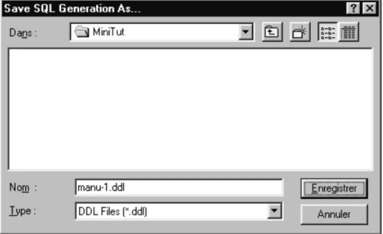
There are several ways in which this conceptual schema can be translated into table and column structures. For now, we have no special requirements as far as performance, or any other consideration, are concerned. We will be happy with an unsophisticated translation of this schema into SQL commands. This translation can be done in a straightforward way through the command
Transform / Quick SQL. DB-MAIN simply asks you, with the standard file
dialog box, in which file you want the SQL program to be stored. By default, the file will be named manu-1.ddl, following the name of the project (Fi-gure 1.17).
Figure 1.17 - The SQL program that is being generated from the conceptual schema will be saved as manu-1.DDL file.
Now, we go back to the Project window. We observe that a new product has been made available. The slightly different icon shape indicates that this new document is a text file called manu-1.ddl. Obviously, this is the SQL pro-gram we just generated in the last step.
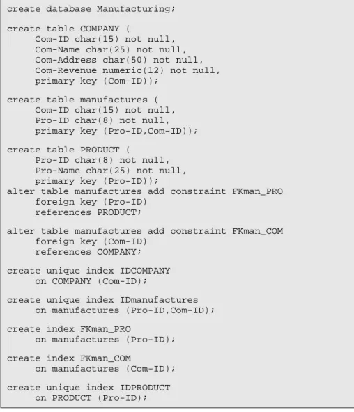
We can examine the contents of this text file by double-clicking on its icon. A new text window opens, showing the SQL code implementing the conceptual schema. It should read like in Figure 1.19.
Figure 1.18 - Now, the project window includes two products, namely the con-ceptual schema and the SQL program that derives from it.
Figure 1.19 - The contents of the manu-1.ddl text file can be examined by double-clicking on its icon in the project window.
create database Manufacturing;
create table COMPANY (
Com-ID char(15) not null, Com-Name char(25) not null, Com-Address char(50) not null, Com-Revenue numeric(12) not null, primary key (Com-ID));
create table PRODUCT (
Pro-ID char(8) not null, Pro-Name char(25) not null, Com-ID char(15) not null, primary key (Pro-ID));
alter table PRODUCT add constraint FKmanufactures foreign key (Com-ID) references COMPANY;
create unique index IDCOMPANY on COMPANY (Com-ID); create unique index IDPRODUCT on PRODUCT (Pro-ID); create index FKmanufactures on PRODUCT (Com-ID);
To be quite precise, this SQL program will not necessarily be executable on all machines, and would probably need some syntactic adjustements. For ins-tance, dashes ("-") are not allowed by most SQL DBMS, and should be repla-ced by, say, underscores ("_"). We will see later how this kind of problem can be addressed in a systematic way.
In addition, the set of indexes may not be the most efficient one, and would need some refinement. Such decisions relate to physical design, an activity that obviously is far beyond the scope of this first lesson!
1.11 Saving the project
As is natural after working such a long time, we carefully save our work throu-gh command File / Save project (or button) or command File / Save
pro-ject as (or button) in order to make it available for further use.
Figure 1.20 - The whole project is saved on disk.
By default, the project is saved as file manu-1.lun. We validate the opera-tion through the button OK.
The *.lun extension is typical to the saved DB-MAIN projects, so do not use them for other files.
1.12 Quitting DB-MAIN
It is now time to exit from the DB-MAIN tool by command File / Exit. We have built our first SQL database, and we are now able to build other sim-ple SQL databases just by applying the basics that have been presented in this lesson.
Key ideas of Lesson 1
1. A CASE (Computer-Aided Software Engineering) tool is a software that allows a developer to draw the conceptual schema of an application domain, then to generate the SQL tables that represent this application domain. 2. The application domain is that part of the real world about which we want to
collect, maintain and process information. This information will be represen-ted by data stored in the database of the application domain.
3. A database is a collection of data that codes facts about the application domain. At the present time, most databases are organized into relational tables. A table is made up of columns; some of which can be declared its pri-mary key. Indexes can be associated with each table.
4. A conceptual schema is the computer-independent description of the facts that make up an application domain. It comprises entity types, attributes, relationship types (or rel-types) and identifiers. An entity type describes a class of significant concrete or abstract objects of the application domain. An attribute represents a property common to the entities of a given type. A rel-type represents a class of associations between entities.
5. The CASE tools can turn a conceptual schema into a database schema. It sto-res both schemas so that they can be used again later on.
Summary of Lesson 1
• In this first lesson, we have studied some important concepts: - the concept of CASE tools
- projects and schemas
- entity types, relationship types, attributes and identifiers - conceptual schemas
- SQL expression of a conceptual schema
• We have also learned to:
- run the DB-MAIN CASE tool
- create a new project: File / New project
- create a new schema: Product / New schema
- define an entity type: New / Entity type
- define an attribute: New / Attribute
- define a relationship type: New / Rel-type - define an identifier: New / Group
- add a semantic description:
- save the current project: File / Save as
- save the current project: File / Save
- produce SQL code: Quick DB / SQL
or Transform / Quick SQL - exit from DB-MAIN: File / Exit
• We have produced two types of files: - saved projects (*.lun)
Exercises for Lesson 1
Define a project, a conceptual schema and generate an SQL database creation program for each of the situations described below.
1.1 The small database we developed in this lesson was based on the hypo-thesis that a product is manufactured by one company only (cardinality 1-1). Now, consider that a product can be produced by any number of
companies (i.e., by 0, 1, 2, or more companies). Change the schema
ac-cordingly. Don’t save this project.
1.2 Customers buy products in such a way that each customer can buy any number of products and each product can be bought by an arbitrary number of customers. Imagine some natural attributes for the entity ty-pes. Call this project SALES1 and save it.
1.3 Students belong to classes: each student belongs to exactly one class (no less, no more), while a class comprises any number of students. Each student can be registered in any number of courses while any number of students can be registered for a given course. Imagine some natural at-tributes for the entity types. Call this project STUDENT1 and save it. 1.4 Complete the MANU-1 project by considering countries to which
pro-ducts are exported.
Don't save the modified project (we will make use of the original ver-sion in further lessons), unless you give it another name.
Lesson 2
A closer look at schemas
Objective
This is an easy and relaxing lesson (just playing with existing schemas!). It presents some useful schema display formats and the way to use them.
Preliminary checking
In this lesson, we will use the project MANU-1 (file manu-1.lun) that has been created in Lesson 1, and the LIBRARY project (or its French equivalent
BIBLIO) that comes with the DB-MAIN software.
2.1 Starting Lesson 2
Let us start DB-MAIN and open the MANU-1 project through the command
Project / Open project or by clicking on the button . When the project is opened, we double-click on the icon of the Manufacturing/Concep-tual schema to display its contents.
For this lesson, we will need some new functions that are offered by the menu, but that are available on a new tool palette as well. We display this new palette through Windows / Graphical tools (Figure 2.1). These tools can be placed anywhere on the screen, for instance under the Standard tool bar.
Figure 2.1 - The graphical tool bar. It can be resized according to your taste.
2.2 On including database schemas into a document
In the first lesson, several figures include a schema, showing the step-by-step construction of the conceptual description of our database. As everybody should have observed, these schemas have been obtained from screen copies. This technique provides nice looking results, but is rather painful (the screen shots have to be processed with an image processing software) and yields huge documents.
The DB-MAIN tool includes a function that copies selected schema objects onto the clipboard in a more concise format (as vector-based objects). So, se-lect all the objects of the schema, then call the Edit / Copy graphic menu item or click on the button in the Graphical tools bar. Then, open a Word or
Powerpoint document, and paste the clipboard contents (use Paste or Paste
Special according to the software).
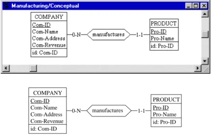
The schema objects appear in the text document as in Figure 2.2 (bottom). The result can be modified as any vector-based graphical object1. From now on, we will use this technique to include schema fragments in this lesson and in the next ones.
Figure 2.2 - Bitmap (top) and vector-based (bottom) schemas as they appear in a text document.
2.3 Graphical views of a schema
In Lesson 1, the schema was represented in a Schema window through graphi-cal objects. There are several other ways to display this schema. They can be classified into graphical views and textual views. This section is devoted to graphical views.
1. In some products, such as MS-Word or FrameMaker, the labels may appear to be too long or too short for the rectangles in which they are enclosed after the schema has been redi-mensioned. This is due to the way Windows redimensions a graphical object: continuously for geometrical components and point by point for texts. In this case, just expand or stretch
1-1 0-N manufactures PRODUCT Pro-ID Pro-Name id: Pro-ID COMPANY Com-ID Com-Name Com-Address Com-Revenue id: Com-ID
Let us first examine a new way of presenting large schemas, namely the
com-pact view. It can be obtained through the View / Graph. comcom-pact command.
The attributes and identifiers are hidden in such a way that only the schema
skeleton appears (Figure 2.3).
Figure 2.3 - The compact graphical view of the MANU-1/Conceptual schema.
Now, we go back to the standard graphical view through View / Graph.
stan-dard, to get the view we have used so far (Figure 2.4). Since this view is the
most useful, it has been given a special button on the Standard tools bar: .
Figure 2.4 - The standard graphical view of the MANU-1/Conceptual schema.
Starting from this standard view, we can derive some simplified forms by using the graphical settings panel (View / Graphical settings) (Figure 2.5). The buttons of the Show Objects block of this panel can be unchecked, which hides the attributes, or the identifiers (called groups in the panel), or both (Fi-gure 2.6). You can also show the attribute types if needed.
Graphical variants exist to represent entity types and rel-types. For instance, we can choose to draw entity type and/or rel-type boxes with round corners instead of square ones by selected rounded shape in the Graphical settings pa-nel (Figure 2.7). These settings are valid for the current schema. They can be useful to distinguish different levels of schemas.
1-1 0-N manufactures PRODUCT COMPANY 1-1 0-N manufactures PRODUCT Pro-ID Pro-Name id: Pro-ID COMPANY Com-ID Com-Name Com-Address Com-Revenue id: Com-ID
Figure 2.5 - The graphical settings panel.
Figure 2.6 - The Standard view without Attributes (top) and without Groups (i.e., without identifiers) but with attribute types (bottom).
1-1 0-N manufactures PRODUCT Pro-ID: char (8) Pro-Name: char (25) COMPANY Com-ID: char (15) Com-Name: char (25) Com-Address: char (50) Com-Revenue: num (12) 1-1 0-N manufactures PRODUCT id: Pro-ID COMPANY id: Com-ID
Figure 2.7 - Round-corner shape and shaded boxes as alternate graphical re-presentations.
A last trick before leaving the graphical views of a schema: how to retrieve a selected object in a schema. Let us suppose that the (small) schema window shows a fragment of a (large) schema. Let us also suppose that an object is selected, somewhere in the schema, but not shown in the window. How to move the window in such a way that the selected object is at the center of this window? Nothing can be simpler: just press the tab key.
What if there is more than one selected object? The tab key brings the next
selected object to the window.
2.4 Textual views of a schema
The contents of a schema can be presented as a pure text as well. In this mode, four formats are available.
The simplest one is the compact view. It shows a mere list of the names of the entity types followed by that of the relationship types (Figure 2.8).
1-1 0-N manufactures PRODUCT Pro-ID Pro-Name id: Pro-ID COMPANY Com-ID Com-Name Com-Address Com-Revenue id: Com-ID 1-1 0-N manufactures PRODUCT Pro-ID Pro-Name id: Pro-ID COMPANY Com-ID Com-Name Com-Address Com-Revenue id: Com-ID
Figure 2.8 - The Text compact view of a schema
This list is a sort of dictionary. It can be obtained through the command View / Text Compact.
The compact view does not display the detail of a schema and can be used as a quick index to locate an object in a large schema.
For a more detailed textual view, try the Standard view. It can be obtained through the command View / Text Standard, and presents the current schema as in Figure 2.9. Since it is frequently used, it can also be obtained through a specific button on the Standard tools bar: .
Figure 2.9 - The Text standard view of a schema
Schema Manufacturing/Conceptual COMPANY PRODUCT manufactures Schema Manufacturing/Conceptual COMPANY Com-ID Com-Name Com-Address Com-Revenue id: Com-ID PRODUCT Pro-ID Pro-Name id: Pro-ID manufactures( [1-1] : PRODUCT [0-N] : COMPANY)
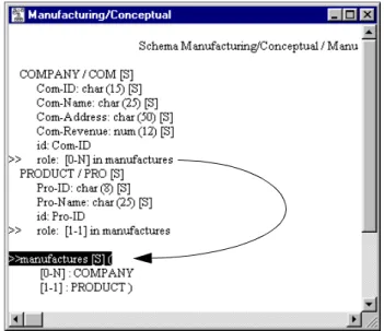
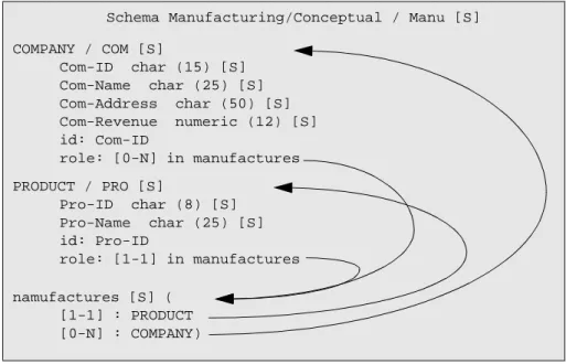
The extended view is an even more complete presentation. In addition to the information of the standard view, the extended view shows, among others, the short names, the type and length of the attributes and the roles in which each entity type appears. The symbol [S] indicates that a semantic description has been associated to the object.
This view is obtained through the command View / Text extended, and ap-pears as in Figure 2.10.
Figure 2.10 - The Text extended view of a schema. The directed arcs show the possible jumps through the hyperlinks activated by a right-button click.
Note that the role lines that appear both in the entity type and rel-type paragra-phs makes it possible to navigate through the whole schema by jumping from an entity type to the relationship types in which it appears, and conversely: - to jump from an entity type to one of its relationship types: click on the line
of the role in the entity type paragraph with the right button of the mouse. - to jump from a relationship type to one of its entity types: click on the line
Schema Manufacturing/Connceptual / Manu [S]
COMPANY / COM [S] Com-ID char (15) [S] Com-Name char (25) [S] Com-Address char (50) [S] Com-Revenue numeric (12) [S] id: Com-ID role: [0-N] in manufactures PRODUCT / PRO [S] Pro-ID char (8) [S] Pro-Name char (25) [S] id: Pro-ID role: [1-1] in manufactures namufactures [S] ( [1-1] : PRODUCT [0-N] : COMPANY)
These hyperlink functions are very handy for large schemas. More on schema navigation later on in Lesson 3.
The last format is the sorted view, which presents an unstructured sorted list of all the names that appear in the schema, together with their type and origin. This view is particularly important for large and complex schemas, specially in reverse engineering activities2. It can be used too when checking names in conceptual analysis. In addition, it is the easiest way to retrieve an object when only its name is known.
The sorted view can be obtained through the command View / Text sorted, and appears as in Figure 2.11.
Figure 2.11 - The Text sorted view of a schema
Two important properties
- Objects that are selected (in white on black) in a view still are selected in any other view in which they appear. For instance, an attribute with a par-ticular name can be retrieved in a schema by using the text sorted view. Now, choosing the standard graphical view allows us to examine this attri-bute in its context.
2. Reverse engineering can briefly be described as the converse of what we did in the first lesson, that is recovering the conceptual schema of an existing database. It involves com-plex techniques and tools that are described in other documents but that will be ignored in
Schema Manufacturing/Conceptual
Com-Address Att. of COMPANY Com-ID Att. of COMPANY Com-Name Att. of COMPANY Com-Revenue Att. of COMPANY COMPANY Entity type manufactures Rel-type
Pro-ID Att. of PRODUCT Pro-Name Att. of PRODUCT PRODUCT Entity type
- Building a schema, or examining, deleting and modifying its components, can be performed whatever the view in which this schema is displayed. For instance, double-clicking on the line of an object in a text view opens the same property box as in a graphical view.
2.5 Application: far jumps through a graphical schema
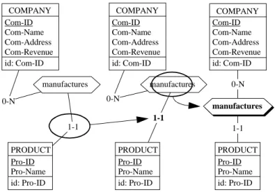
Navigating through a large schema can be fairly tricky. Let us examine the simple following problem: considering entity type COMPANY, show the entity type that plays the other role in rel-type manufactures.In the schema of Figure 2.4, the problem is solved simply by positioning the schema window on entity type COMPANY, then in selecting the other end of rel-type manufactures.
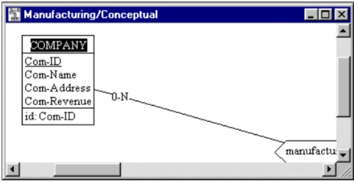
Now, let us consider that these objects are parts of a large schema, in such a way that both entity types are more than one meter apart (Figure 2.12). Re-trieving rel-type manufactures, then entity type PRODUCT gets much more difficult. We have to activate the scroll bars in several directions, fol-lowing very carefully the arcs that make the rel-types. It is easy to confuse two crossing arcs, and to follow the wrong direction.
The solution is to use the right view(s) in the right way:
1. in the Graphical standard view, we select entity type COMPANY (Figure 2.12);
2. we switch to the Text extended view and we click with the right button on the role line "role: [0-N] in manufactures", which sends us to rel-type ma-nufactures (Figure 2.13);
3. in the list of roles of manufactures, we identify the opposite role ([1-1]: PRODUCT) and we click on it with the right button;
4. this sends us to entity type PRODUCT (Figure 2.14);
5. we switch to a graphical view, which shows the selected object3 (Figure 2.15), and voilà!
Figure 2.13 - We reach rel-type manufactures by right-clicking on the role of COMPANY.
Figure 2.14 - The opposite entity type has been found ...
Key ideas of Lesson 2
1. A CASE tool can memorize the products (schemas and generated texts) of a project on secondary memory. They can be opened later on.
2. A fragment of a schema can be incorporated into a text document either as a bitmap image (through PrintScreen key) or, better, as a vector-based drawing. 3. A schema can be displayed under various formats, either graphical or textual.
Each of them shows some or all aspects of the schema objects.
4. The graphical formats are more intuitive, and show the direct environment of an object.
5. The textual formats are more concise, and can show syntactic patterns of the object names.
6. Some textual formats make it possible to jump to distant linked objects. 7. Switching between different formats allows us to quickly navigate through
Summary of Lesson 2
• In this first lesson, we have studied some important concepts: - graphical views of a schema: compact, standard
- text views of a schema: compact, standard, extended, sorted - navigation through the objects of a schema
• We have also learned:
- to open an existing project:
Project / Open project
- to open an existing schema
- to include fragments of a schema into a text:
Edit / Copy graphic
- to select a schema presentation format:
View / Text compact View / Text standard View / Text extended View / Text sorted View / Graph. compact View / Graph. standard
- to give graphical objects rounded corners and shades:
View / Graphical settings
- in a text view, to navigate from entity type to rel-type and from rel-type to
entity type: right button on the role line
- in a graphical view, to get the next selected object in the center of the sche-ma window: tab key
Exercises for Lesson 2
Finding interesting exercises for such a lesson is quite a challenge! If you in-sist, try these; otherwise start the next lesson.
Open the LIBRARY project (or its French equivalent BIBLIO) and its con-ceptual schema Library/Conceptual.
2.1 Examine the semantic description of the objects in the schema. Change and complete some of them.
2.2 Change the position of some attributes and roles in text views. Examine the graphical view and change the position of some objects.
Lesson 3
An even closer look at schemas
Objective
In this sequel to Lesson 2, we study how to manipulate graphical and textual objects, how to change their apparent or actual size, how to navigate through a schema and to generate reports. We also examine various techniques to inspect the objects of a sche-ma.
Preliminary checking
Make sure that the project MANU-1 (file manu-1.lun) created in Lesson 1, and LIBRARY (or its French equivalent BIBLIO) that comes with the DB-MAIN software, are available.
3.1 Starting Lesson 3
We start DB-MAIN, we open the project MANU-1, then the schema Manu-facturing/Conceptual.
3.2 Securing our work
This lesson, as well as the next ones, will lead us to perform various manipu-lations on the current schema, and therefore to spoil its initial shape and con-tents. Of course, when this happens we could restore the original version that has been saved on disk by File / Open project, but this is rather tedious, espe-cially for large projects.
The save point/rollback technique is much quicker:
- Edit / Save point saves the state of the current schema (or button ), - Edit / Rollback cancels the modifications carried out on the current schema
since its last save point; in other words, it restores the state of the schema when the last save point was issued.
Three important rules:
1. There is only one active save point for the schema, but each schema of the project can have its own independent save point.
2. A save point cannot restore a schema that has been deleted (use File / Save
as instead).
3.3 Manipulating the graphical components of a schema
The position of the objects of a schema can be changed by selecting anddrag-ging them in the usual way. Several objects can be selected (or deselected) by
pressing the shift key when selecting, or by drawing a selection rectangle with the mouse, and moved simultaneously.
Moving objects
Moving objects in their window obeys the general Windows rules:
- selected objects are moved by dragging them in the window space; - selected objects are moved by pressing the cursor keys (← ↑ → ↓); - small-step moves are obtained by pressing the cursor keys while pressing
the Ctrl key;
- using the scroll bars moves the window in the four directions.
The Move mode designates the way DB-MAIN reacts when an object is mo-ved on the screen: does it move the object only (independent mode), or does it reposition the connected objects as well (dependent mode)? This mode can be set either in the Graphical settings panel (Independent button) or through the INDEP. button on the Graphical tools bar: .
In the Dependent mode, the graph is adjusted as follows (Figure 3.1 left): - when an entity type is moved, its relationships types and their roles are
moved proportionally and redrawn;
- when a relationship type is moved, its roles are moved too, - when a role is moved, nothing else is redrawn.
In the Independent mode, the graph is adjusted as follows (Figure 3.1 right): - when an object (entity type, relationship type, role) is moved, nothing
Figure 3.1 - Moving rel-type manufactures in the dependent mode (left) and in the independent mode (right).
Aligning objects
After a while, a schema may look like spaghetti, and we might want to put some order among its components. A first nice feature is the rel-type Align action which allows us to align a role or a relationship type according to its connected objects. We can get this effect by clicking on the object (role or rel-type) with the right button of the mouse (Figure 3.2).
To align a larger set of objects, we will make use of the View / Alignment command, that provides us with eight operators, four for vertically aligning the objects and four for horizontal alignment. They are also available on the
Gra-phical tools bar (Figure 3.3).
In the horizontal dimension, we can align objects on their left side, on their right side, we can center them and we can distribute them horizontally at equal distance.
In the vertical dimension, we can align objects on their top side, on their bot-tom side, we can center them and we can distribute them vertically at equal distances. 0-N 1-1 manufactures 1-1 0-N manufactures PRODUCT Pro-ID Pro-Name id: Pro-ID PRODUCT Pro-ID Pro-Name id: Pro-ID COMPANY Com-ID Com-Name Com-Address Com-Revenue id: Com-ID COMPANY Com-ID Com-Name Com-Address Com-Revenue id: Com-ID
Figure 3.2 - Aligning roles (center) and relationship types (right) by clicking with the right button of the mouse.
Figure 3.3 - The eight object alignment operators.
Horizontal object moves : align to left
: align to right
: center horizontally between left and right : distribute evenly between left and right
Vertical object moves : align to top
: align to bottom
: center between top and bottom
: distribute evenly between top and bottom 1-1 0-N manufactures 0-N 1-1 manufactures 1-1 0-N manufactures PRODUCT Pro-ID Pro-Name id: Pro-ID PRODUCT Pro-ID Pro-Name id: Pro-ID PRODUCT Pro-ID Pro-Name id: Pro-ID COMPANY Com-ID Com-Name Com-Address Com-Revenue id: Com-ID COMPANY Com-ID Com-Name Com-Address Com-Revenue id: Com-ID COMPANY Com-ID Com-Name Com-Address Com-Revenue id: Com-ID
Two comments:
1. Horizontal means that the objects are moved horizontally to reach their fi-nal position (the same for the vertical direction).
Figure 3.4 - The four arc alignment operators.
Figure 3.5 - How to draw a source rel-type (top) with staircase style with just a mouse click. Arc alignment : horizontal staircase : vertical staircase : top corner : bottom corner 1-1 0-N R B A 1-1 0-N R B A 1-1 0-N R B A 1-1 0-N R B A 1-1 0-N R B A
2. When the objects are distributed evenly, the distance is evaluated between the edges of the objects, not between their centers. This provides a natural positionning of roles and rel-types between their entity types.
The last four alignment operators (Figure 3.4) are dedicated to users who are found of staircase rel-types. Since an image is worth one thousand words, we suggest you had a look at Figure 3.5.
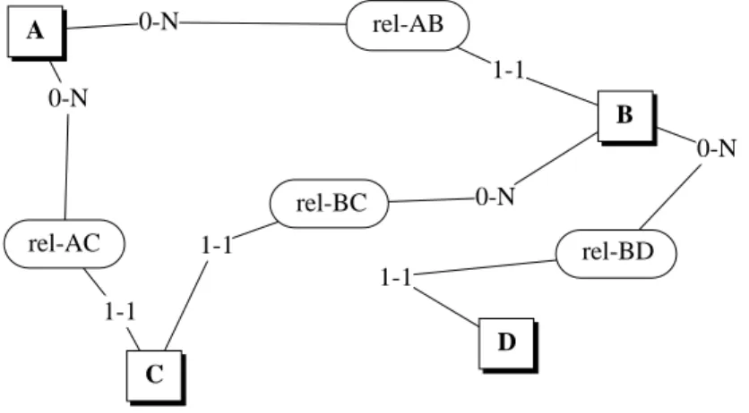
The best way to get acquainted with these operations is to play with a disali-gned schema such as that of Figure 3.6, which is available in project Manu-3.lun, schema Alignment.
Figure 3.6 - This schema obviously suffers from a severe disalignment di-sease. Cure it.
Zooming in and out
For large schemas, a zooming function is available to help fit a larger or a smaller portion of the schema in the Schema window (zoom out), or to exami-ne tiny details (zoom in). This function is available in the Graphical settings
panel (Figure 2.5) and in the Graphical tools bar (Figure 2.1) through the
fol-lowing buttons:
expands the schema representation by 10%; shrinks the schema representation by 10%;
1-1 0-N rel-BC 1-1 0-N rel-BD 1-1 0-N rel-AC 1-1 0-N rel-AB D B C A
sets the zoom factor by specifying its exact value; the fit value adjusts the zoom factor so that the schema fits in the schema win-dow.
Fonts
The font, font size and style of the object names can be changed through the command Edit / Change font. You can get a more compact view by de-creasing the character size.
Grids
Organizing large schemas may require the use of the Grid function, which draws lines that decompose the graphical space into equal size pages (see the
Grid format block in the Graphical settings panel, Figure 2.5). The page size
can be standard (A3, A4, Letter), with portrait or landscape orientation, com-pliant with the current printer, or customized.
The Reduce function
This is a way to change (shrink or expand) the actual size and position of each object of the current schema by a certain factor. It seems similar to the Zoom function, but the latter only defines how close you are from the schema, while leaving the objects themselves unchanged. The following table should make the differences betwen Reducing and Zooming more explicit.
Colors
Normally, all the objects in a schema are drawn, and their names are written, in black. You can change this by selecting objects, then giving them another
color. Use command Edit / Color selected or click on the button in the
Standard tools bar to give them the current color. This color can be changed
by the command Edit / Change color.
objects object appearance grid grid appearance
zoom out by 50% unchanged reduced by 50% unchanged reduced by 50% reduce by 50% reduced by 50% reduced by 50% unchanged unchanged
Marking objects
This is a very simple and powerful means to define persistent subsets of ob-jects in a schema. Marking obob-jects is obtained by first selecting the obob-jects, then asking Edit / Mark selected or clicking on the button in the Standard
tools bar. To unnmark objects, just mark them again. Marked objects are
drawn with specific attributes (Figure 3.7):
- a marked entity type is shaded (unless it was already shaded, in which case it is unshaded) and its name is written in boldface;
- a marked rel-type is shaded (unless it was already shaded, in which case it is unshaded) and its name is written in boldface;
- a marked attribute is written in boldface;
- a marked identifier (or group) is written in boldface; - a marked role is written in boldface.
The main difference between selecting and marking objects is that marking is a permanent state while a selection is volatile. Closing a schema and saving it on disk keep all the marks until we change them explicitly.
Figure 3.7 - Entity type PRODUCT, rel-type manufactures, attributes
Com-Address and Com-Revenue, role PRODUCT of manufactures
and identifier Pro-ID are marked.
Retrieving all the marked objects in a schema cannot be simpler: just select them by Edit / Select marked. To unmark all the marked objects of a schema, select them as above, then mark them again.
In fact, it is possible to define up to 5 different sets of marked objects. Such a set corresponds to a marking plane. All the marking operations are carried out in the current marking plane. Changing the current plane is done through a special button in the Standard tools bar:
1-1 0-N manufactures PRODUCT Pro-ID Pro-Name id: Pro-ID COMPANY Com-ID Com-Name Com-Address Com-Revenue id: Com-ID
When a combination of marked and unmarked objects are set to marked, the result is that they are all marked. This makes it possible to combine the objects marked in two planes into a third one:
1. transfer from plane 1 to plane 3: choose the first plane, select the marked objects, choose the third plane and mark the selected objects,
2. transfer from plane 2 to plane 3: choose the second plane, select the mar-ked objects, choose the third plane and mark the selected objects.
If no objects are marked eventually, this means that planes 1 and 2 were iden-tical. In this case, just do step 1 again.
There are numerous applications of marking planes:
- in a large schema which is still in a validation phase, objects which are already checked are marked; the schema is completed when all objects are marked;
- objects which have been given a semantic description are marked; the sche-ma is completely documented when all the objects are sche-marked;
- in a schema that comprises objects from different sources, each source is marked in a different marking plane; an object can be marked in more than one plane1;
- marked objects can be manipulated by DB-MAIN processors (as we will see later on)
- some DB-MAIN processors can return marked objects (as we will see later on).
Auto-draw
If the layout of a schema does not fit your taste, you can ask DB-MAIN to sug-gest a better spatial arrangement through the command View / Auto-draw. This function is particularly useful for large schemas that have not been ente-red graphically (through the reverse engineering extractors for instance)2. If
Auto-Drawing a schema does not produce a satisfying result, try auto-drawing
again. Generally, you will need to fine-tune the layout manually.
1. For this aim, a view schema is a much better means to define an arbitrary number of sub-sets of objects. They will be studied in Lesson 12.
2. This function is at its best for large and complex schemas. It does not provide satisfying results with small schemas. Before using it, it can be wise to save the schema state through
Using a larger schema
To get a better feeling of the usefulness of the various views, we switch to ano-ther project. We close the current one (command File / Close project), and we open the LIBRARY project (command File / Open project) and its con-ceptual schema. Now we experiment with each view, and try to figure out the meaning of the components of this schema, which obviously describes the ma-nagement of a scientific library. Its contents include many more modeling characteristics that will be discussed later.
Last observations
We observe that:
- switching from a view to another one is immediate, and can be asked for at any time;
- the operations of the tool are independent of the view through which they are executed;
- an object that is selected (highlighted) in a view still is selected when we switch to another view;
- if several schemas of a project are opened (more on this later on), they can be displayed in different views.
3.4 Navigation through textual views
When a schema is small, it spans one or two screens only. Retrieving an object in such a schema needs no special skill nor any special tool. The problem is less trivial when the schema is larger, and is several dozens of screens large (large schemas can include thousands of entity types and rel-types): browsing through such a schema can be time consuming and does not garantee that the objects we are looking for will be found quickly, if ever.
Retrieving a specific object can often be made easier by working first on the
Text compact and Text sorted views, using them as some kind of
dictiona-ries, then switching to the standard graphical or text views when the object of interest has been found.
Another useful tool for object retrieval in context is the navigation feature of DB-MAIN. To illustrate them, we need a larger schema, such as LIBRARY.
We display it in the Text extended view, and we reduce the Schema window a little bit to simulate a large schema in a too small window.
Let us experiment the navigation capabilities of DB-MAIN. Unless told othe-rwise, the following manipulations are valid for the Text standard and Text
extended views.
- We select the COPY entity type by clicking on its name; we observe that each line in which the name COPY appears (i.e., each instance of COPY) is tagged with symbols ">>"; such is the case for each role in which COPY appears;
- If we press the TAB key; the next tagged instance of COPY appears in the center line of the Schema window; this allows the cursor to jump to each of the relationship types in which COPY takes part;
- We click with the right button on a line describing a role in which COPY appears, in a rel-type paragraph; the COPY entity type is then selected; the right button acts as a go home button;
- In the Text extended view, we click with the right button of the mouse on a role in which COPY appears, in its entity type paragraph, then click; the relationship type of the role is then selected
In Figure 3.8, the navigation rules are shown on the small project Manu-1.
3.5 Reordering attributes and roles
Though the order in which attributes (and roles) appear in the textual and gra-phical views does not matter in most situations, you may want to change this order.
To change the position of an attribute (graphical and text views), select it, then
- press the Alt + ↑ keys3 to move it one position up,
- press the Alt + ↓ keys to move it one position down (Figure 3.9). To change the position of a role (text views), select it, then - press the Alt + ↑ keys to move it one position up,
Figure 3.8 - Navigating in the Text extended view of a schema of project
Manu-1 with the right button of the mouse.
There are other ways to reorganize the attributes of an entity type, but they re-quire more sophisticated functions (namely schema transformations) that will be studied later.
Figure 3.9 - Changing the order of the attributes with Alt + ↓↑.
Schema Manufacturing/Conceptual / Manu [S]
COMPANY / COM [S] Com-ID char (15) [S] Com-Name char (25) [S] Com-Address char (50) [S] Com-Revenue numeric (12) [S] id: Com-ID role: [0-N] in manufactures PRODUCT / PRO [S] Pro-ID char (8) [S] Pro-Name char (25) [S] id: Pro-ID role: [1-1] in manufactures namufactures [S] ( [1-1] : PRODUCT [0-N] : COMPANY) COMPANY Com-Name Com-ID Com-Revenue Com-Address id: Com-ID COMPANY Com-ID Com-Name Com-Address Com-Revenue id: Com-ID
3.6 Generating reports
A decent CASE tool must produce external documents that can be printed on paper. This one does it too. Several kind of reports can be of interest, ranging from simple object lists to sophisticated documents including a table of con-tents, an index and footnotes. Though DB-MAIN can produce such docu-ments, we will show how to generate simple outputs. Three formats are available from the menus through the command File / Report.
Figure 3.10 - Generating a simple text report.
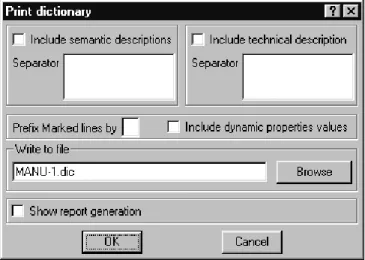
1. Textual view: the schema must be displyed in a text view (for instance with button ). Its representation is sent to a file with some format options that are set through the Print dictionary panel (Figure 3.10). This function pro-duces a *.dic plain ASCII file.
This panel allows us to specify - the output file,
- whether we want the semantic description to be included,
- what character string will be included just before each semantic descrip-tion (a tab control can be used to clearly separate it from the object des-cription4),
- how the lines of marked objects are tagged. We will ignore the other parameters for now5.
Formatting the output text with a text/document processor can provide re-ports such as that of Figure 3.11.
2. RTF: the schema is saved as a formatted RTF document. Various options are available6.
3. Custom: the schema is processed through a customized Voyager 2 pro-gram7.
For immediate needs, you can directly send the current schema to the printer, be it in graphical or textual view, through command File / Print. The printer can be chosen and configured through File / Printer setup as usual.
There are other ways to produce reports. Let us remember one of them: the
Copy graphic function, that allows us to include fragments of schemas into
standard texts (Section 2.2).
3.7 Copying objects
When building a schema, it can happen that several entity types have to be gi-ven similar attributes, or that the schema includes parts that are almost the sa-me. Instead of entering the similar objects manually, it could be more convenient to copy the original fragment, then to modify the copy.
The procedure is as expected:
1. select the components to copy and put them on the clipboard (ctrl+C or
Edit / Copy);
2. paste them in the schema (ctrl+V or Edit / Paste);
5. For those who do want to know: Include dynamic peoperties values means that user-defi-ned object properties are to be included in the report (see Lesson 16) and Show report generation means that we want the report and its generation process to appear in the project windows (in fact in the process history). In this lesson, the effect of checking this button will be to show the report as a product in the project window.
6. Check that the DB-MAIN directory includes the files XXXXX and XXXXX. You can define their paths through File / Configuration.
7. We will tell some words about these programs later on. For now, it suffices to know that Voyager 2 is the programming language of DB-MAIN allowing its users to develop their
Figure 3.11 - A simple text report.
3. if the the pasted objects are attributes, first select an entity type, a rel-type or an attribute; the pasted objects will be inserted after this insertion point (Figure 3.12).
If needed, DB-MAIN makes the names of the pasted objects unique through the addition of a small suffix.
____________________________________________________________
Dictionary report
Project MANU-1
____________________________________________________________
Schema Manufacturing/Conceptual
A simple example of conceptual database schema used in the first lessons of the DB-MAIN tutorial. This schema has been created on December 15, 1998.
* COMPANY A registered business organization with which we have had commercial contacts for less than 5 years.
Com-ID Internally assigned company Id. Com-Name Official name of the company. Com-Address Main address of the company.
Com-Revenue The total net income of company for the last fiscal year.
id: Com-ID
* PRODUCT A product of interest for our company. Pro-ID Internally assigned product Id.
Pro-Name The conventional name of the product. id: Pro-ID
* manufactures ( Specifies which products are manufactu-red by each company.
[0-N] : COMPANY [1-1] : PRODUCT )
Note. Copying attributes to define near similar objects can be an evidence of a more complex situation, where entity types appear to be subtypes of each other, or to have a common supertype. These structures will be studied in Section 8.2. ν
Figure 3.12 - It appears that SALESMAN must be given attributes similar to
Name and Address of CUSTOMER (left). Select the latter, type ctrl+C, select
EmpID of SALESMAN then type ctrl+V (right).
3.8 Inspecting objects
Examining the properties of the objects in a schema, or even the schema or the project themselves, is quite easy. We double-click on the object (in any text or graphical view) and its property box opens. To read its semantic descrip-tion, we click on the Sem. button, which opens the semantic description win-dow.
If we have to examine a large number of objects, this procedure may appear tedious, and even painful. There exist two quicker ways to inspect the proper-ties of the objects.
First, opening the semantic description window can be done by selecting the object and clicking on the SEM button in the Standard tools bar .
The second way is much more powerful, and uses a new DB-MAIN feature called the Property box. It is opened through command Window / Property
box, and appears as in Figure 3.13.
This box is permanent until it is explicitly closed. It shows in real time all the properties of the current object, i.e., the object which is currently selected. Simply select another object, and the box shows the properties of this object.
SALESMAN EmpID id: EmpID CUSTOMER CustID Name Address Number Street City id: CustID SALESMAN EmpID Name Address Number Street City id: EmpID CUSTOMER CustID Name Address Number Street City id: CustID
Figure 3.13 - The contents of the Property box when attribute Com-Revenue is selected.
The Property box has three panels. The second one shows the semantic cription of the selected object (Figure 3.14). Now, reading the semantic des-cription of a series of objects can be done by merely selecting each of these objects.