HAL Id: tel-01288217
https://tel.archives-ouvertes.fr/tel-01288217
Submitted on 14 Mar 2016HAL is a multi-disciplinary open access archive for the deposit and dissemination of sci-entific research documents, whether they are pub-lished or not. The documents may come from teaching and research institutions in France or abroad, or from public or private research centers.
L’archive ouverte pluridisciplinaire HAL, est destinée au dépôt et à la diffusion de documents scientifiques de niveau recherche, publiés ou non, émanant des établissements d’enseignement et de recherche français ou étrangers, des laboratoires publics ou privés.
High-resolution modelling with bi-dimensional shallow
water equations based codes : high-resolution
topographic data use for flood hazard assessment over
urban and industrial environments
Morgan Abily
To cite this version:
Morgan Abily. High-resolution modelling with bi-dimensional shallow water equations based codes : high-resolution topographic data use for flood hazard assessment over urban and industrial envi-ronments. Other. Université Nice Sophia Antipolis, 2015. English. �NNT : 2015NICE4121�. �tel-01288217�
UNIVERSITE NICE-SOPHIA ANTIPOLIS
ECOLE DOCTORALE STIC
SCIENCES ET TECHNOLOGIES DE L’INFORMATION ET DE LA
COMMUNICATION
T H E S E
pour l’obtention du grade de Docteur en Sciences
de l’Université Nice-Sophia Antipolis
Mention: Automatique, Traitement du Signal et des Images
présentée et soutenue par
Morgan ABILY
High-resolution modelling with bi-dimensional shallow water equations based
codes – High-resolution topographic data use for flood hazard assessment
over urban and industrial environments –
Thèse dirigée par Philippe GOURBESVILLE,
co-encadrée par Claire-Marie DULUC & Olivier DELESTRE soutenue le 11 décembre 2015
Jury:
M. Shie-Yui Liong, Professeur - National University of Singapore Rapporteur M. Nigel Wright, Professeur - De Montfort University Leicester Rapporteur Mme. Nicole Goutal, Directeur de recherches - Lab. d'Hydraulique de Saint Venant, EDF R&D Examinateur Mme. Claire-Marie Duluc, Ingénieur/chercheur et chef de Bureau - IRSN Examinateur M. Olivier Delestre, Maître de conférence - Université Nice Sophia Antipolis Examinateur
Mme. Nathalie Bertrand, Ingénieur/chercheur - IRSN Invitée
M. Philippe Audra, Professeur - Université Nice Sophia Antipolis Président du jury M. Philippe Gourbesville, Professeur - Université Nice Sophia Antipolis Directeur de thèse
A
CKNOWLEDGMENT
Among many reasons I have to express my thank to them, I would like here to thank Philippe Gourbesville and Claire-Marie Duluc for pushing me to work on this thesis project. They gave me the chance to review the work I have accomplished during my first years of practice as a research engineer at IRSN and Polytech. It is an invaluable luxury.
I would like to express my thanks to the jury of this thesis and particularly to the reviewers for their commitment and valuable feedbacks.
I am grateful to the two colleagues with whom I work with since our CEMRACS 2013 collaboration: Olivier Delestre and Nathalie Bertrand. This thesis project started after the CEMRACS summer school and was an extra workload for them as well.
Part of the material used in this theses have been kindly provided by Nice Côte d’Azur Metropolis for research purpose.
This work was granted access to (i) the HPC and visualization resources of "Centre de Calcul Interactif" hosted by "Université Nice Sophia Antipolis" and (ii) the high performance computation resources of Aix-Marseille Université financed by the project Equip@Meso (ANR-10-EQPX-29-01) of the program "Investissements d'Avenir" supervised by the Agence Nationale pour la Recherche.
Technical support for codes adaptation on high performance computation centers has been provided by Fabrice Lebas, Yann Richet, Hélène Coullon, Christian Laguerre and Minh-Hoang Le.
I also take this opportunity to thank the colleagues from BEHRIG and I-CiTy laboratory I had the pleasure of spending time with these past years. I would like to thanks as well the numerous scientists (from experienced ones to interns) with whom I had the chance to be in touch, exchange and collaborate regarding this work. Lastly, I am thankful to my family and friends. Dany, Didier, Maité, Eugénie, Bernard, Cynthia, Shéba, Tibo, Sébastien, Steph, Alex(s) and Mag, the love and friendship I receive from you is the best daily support one can dream of.
N
OTE TO THE READER
This PhD work started in November 2013, results from the research framework built from the collaborative activities initiated in 2011 between the Institute for Radioprotection and Nuclear Safety (IRSN, Institut de Radioprotection et de Sûreté Nucléaire) and the water department of the Engineering school Polytech Nice Sophia. Two main topics were defined for the research work conducted during this collaboration.
Need for runoff modelling with highly detailed information at industrial site scale. The IRSN wanted to test a specific approach for runoff hazard concern that has been specifically enhanced in the guide for protection of basic nuclear installation against flooding elaborated by the IRSN for the French Nuclear Safety Authority (ASN, 2013). In the guide, a specific runoff Reference Flood Situation (RFS) states that a nuclear installation has to be able to cope with a one hour long rainfall event of one over hundred years return period. IRSN wanted to test feasibility of standard 2D Shallow Water Equations (SWEs) based numerical tools for the runoff RFS. Spreading of High-Resolution (HR) topographic information techniques goes in this direction of a HR dataset (e.g. Light Detection and Ranging or imagery based) easily available for a specific study purpose. Consequently, hydraulic numerical modelling community increasingly uses Digital Elevation Models (DEM) generated from airborne technologies for urban flooding modelling. For a purpose like local runoff flood risk modelling over an industrial site which is a complex environment, added value of High-Resolution (HR) topographic data use that describes in detail the physical properties of the environment was interesting to test. Moreover, Runoff flow paths influencing above-ground features are not equally represented in DEM generated based on LiDAR and photogrammetric data. Lastly, feasibility of HR data in standard 2D numerical modelling tools might be challenging. Possibilities and challenges of these surface features inclusion in highly detailed 2D runoff models for runoff flood hazard assessment deserve a specific consideration and were therefore the key stone which motivated us to work on this thesis.
Need to check uncertainties of the High-Resolution overland flow models - Even though HR classified datasets have high horizontal and vertical accuracy levels (in a range of few centimeters), this data set is assorted of errors and uncertainties. Moreover, in order to optimize models creation and numerical computation, hydraulic modellers make choices regarding procedure for this type of dataset use. These sources of uncertainties might produce variability in hydraulic flood models outputs. Addressing models output variability related to model input parameters uncertainty is an active topic that is one of the main concern for practitioners and decision makers involved in the assessment and development
of flood mitigation strategies. IRSN and Polytech Nice Sophia wish to strengthen the assessment of confidence level in these deterministic hydraulic models outputs.
S
UMMARY
High-resolution (infra-metric) topographic data, including LiDAR data and photogrammetric based classified data, are becoming commonly available at large range of spatial extent, such as municipality or industrial site scale. This category of dataset is promising for High-Resolution (HR) Digital Elevation Model (DEM) generation, allowing inclusion of fine above-ground structures (walls, sidewalks, road gutters, etc.), which might influence overland flow hydrodynamic in urban environment. DEMs are one key input data in Hydroinformatics for practitioner willing to perform free surface hydraulic modelling using standard 2D Shallow Water Equations (SWEs) based numerical codes (e.g. modeller wishing to assess flood hazard). Nonetheless, several categories of technical and numerical challenges arise from this type of data use with standard 2D SWEs numerical codes.
Objective of this thesis is to tackle possibilities, advantages and limits of High-Resolution (HR) topographic data use within standard categories of 2D hydraulic numerical modelling tools for flood hazard assessment purpose.
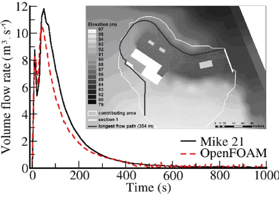
Review of concepts regarding 2D SWEs based numerical modelling and HR topographic data are presented. Methods to encompass HR surface elevation data in standard modelling tools are tested and evaluated. Two types of phenomena generating flooding issues are tested for High-Resolution modelling: (i) intense runoff and (ii) river flood event using in both cases LiDAR and photo-interpreted datasets. Three scales of spatial extent are tested, from a small industrial site scale to a city district scale (Nice low Var valley, France). In this thesis, test studies are performed using a wide range of categories of standard numerical modelling tools based on 2D SWE, from commercial (Mike 21, Mike 21 FM) to open source (TELEMAC 2D, FullSWOF_2D) codes. Comparison is performed with 2D SWEs simplified approaches (diffusive wave approximation using Mike SHE code) and with Navier-Stokes volume of fluid resolution approach (Open FOAM code). Tools and methods for assessing uncertainties aspects with 2D SWEs based models are developed and tested to perform a Global Sensitivity Analysis (GSA) related to HR topographic data use.
Chapter 1 of this thesis introduces state of the art of HR topographic data gathering techniques considering their possibility for a HR description of industrial and urban environment. Moreover, chapter 1 summarizes the background of the theoretical framework of SWEs, in order to raise questions up regarding validity of the approach of 2D SWEs based modelling over complex environments. As the framework of this type of application is different from the one for which SWEs have originally been designed for, the expected limits that might be encountered for HR topographic data use in standards codes are enhanced.
Indeed, if from a practical point of view, codes relying on approximation of SWEs are already commonly used for urban environment overland flow modelling, theoretical questions arise and remain open regarding several conceptual and mathematical aspects. Mainly, due to high gradient occurrences, boundary conditions and initial condition are seldom properly known.
In chapter 2, three case study are used to give a proof of concept of HR topographic data use feasibility, (i) to produce a HR DEM for intense flood simulations in complex environment, and (ii) to integrate this HR DEM information in standard 2D SWEs based codes. Feasibility, performances and relevance of the HR modelling are evaluated with a selection of different codes approximating the 2D SWEs based on various spatial discretization strategies (structured and non-structured) and with different numerical approaches (finite differences, finite elements, finite volumes). A comparison is conducted over computed maximal water depth and water deep evolution. The results confirmed the feasibility of these tools use for the studied specific purpose of HR modelling. Tested categories of 2D SWEs based codes, show in a large extent similar results in water depth calculation under important optimization procedure. Actually, major requirements were involved to get comparable results with a reasonable balance/ratio between mesh generation procedure - computational time - numerical parameters optimization (e.g. for wet/dry treatment).
The inclusion of detailed/thin features in DEM and in hydraulic models lead to considerable differences in local overland flow depth calculations compared to HR models that do not describe the industrial or urban environment with such level of detail. Moreover, added value of fine features inclusion in DEM is clearly observed disregarding resolution used for their inclusion (either 0.3 m or 1 m). Indeed, tests to include fine features (extruding their elevation information on DEM), through an over sizing their horizontal extent to 1 m, lead to good results with respect to their inclusion at a finer resolution.
LiDAR and photo-interpreted HR datasets are tested to compare their ease of use for HR DEM devoted to hydraulic purpose elaboration. Results point out differences, notably regarding ways and possibilities to integrate HR topographic dataset in 2D SWEs based codes. Moreover, due to meshing algorithm properties, the over constraints created by the density of vectors (in case of a HR urban environment) lead to errors and difficulties for non-structured mesh generation. For these reasons, the use of a non-structured mesh representing the HR DEM is found to be a more efficient compromise.
Chapter 3 consists on a focus on uncertainties related to model inputs, and more specifically on uncertainties related to one type of inputs: HR topographic data use and inclusion in 2D SWEs based codes. The aim is:
(i) to be a proof of concept of spatial Global Sensitivity Analysis (GSA) applicability to 2D flood modelling studies using developed method and tools and implementing them on High Performance Computing (HPC) structures;
(ii) to quantify uncertainties related to HR topographic data use, spatially discriminating relative weight of uncertainties related to HR dataset internal errors with respect to modeller choices for HR dataset integration in models.
The Uncertainty Analysis (UA) leads to conclusive results on: output variability quantification, nonlinear behavior of the model, and on spatial heterogeneity. The considered uncertain parameters related to the HR topographic data accuracy and to the inclusion in hydraulic models, influence the variability of calculated overland flow maximal water depth is found to be considerable. This stresses out the point that even though hydraulic parameters are assumed to be fully known in our simulations, the uncertainty related to HR topographic data use cannot be omitted and needs to be assessed and understood.
Sensitivity indices (Sobol) are calculated at given points of interest, enhancing the relative weight of each uncertain parameter on variability of calculated overland flow. Sobol index maps production is achieved. The spatial distribution of Si illustrates the spatial variability and the major influence of the modeller choices, when using the HR topographic data in 2D hydraulic models with respect to the influence of HR dataset accuracy.
T
ABLE OF CONTENTS
Introduction ... 15
Chapter I - Theoretical background ... 21
Part. 1. High-Resolution topographic data in urban environment ... 24
1.1 LiDAR ... 24
1.2 Photogrammetry and photo-interpreted datasets ... 26
1.1.2 Photogrammetry ... 26
1.1.3 Object based classification: photo-interpretation ... 27
1.3 Focus on spatial discretization ... 31
1.4 Feeback for HR topographic data use in 2D urban flood modelling ... 34
Part. 2. Numerical modelling of free surface flow: approximating solution of SWEs ... 36
2.1 From Hypothesis in the physical description of the phenomena to mathematical formulation ... 36
2.1.1 From flow observation to de Saint-Venant hypothesis and mathematical formulation ... 36
2.1.2 Validity and limits of these hypothesis ... 40
2.2 Numerical methods to approach solution of the SWEs system ... 41
2.2.1 Introduction to concepts for a numerical method ... 42
2.2.2 Standard numerical methods ... 44
2.3 Tested commercial numerical codes for HR topographic data use ... 50
Chapter I conclusions: foreseen challenges related to HR topographic data use with 2D SWEs based numerical modelling codes ... 53
Chapter II – Case study of High-Resolution topographic data use with 2D SWEs based
numerical modelling tools ... 55
Part. 3. High-Resolution runoff simulation at an industrial site scale ... 58
3.1 Test case setup ... 61
3.1.1 Presentation of mathematical and numerical approaches ... 61
3.1.2 Site configuration and spatial discretization ... 62
3.1.3 Runoff scenarios and models parameterization ... 66
3.1.4 Performance assessment methodology ... 68
3.2 Results ... 72
3.2.1 Rainfall events scenarios (S1 and S2) ... 72
3.2.2 Initial 0.1 m water depth scenario (S3) ... 77
3.2.3 Indicators of computation reliability ... 81
3.3 Discussion and perspectives ... 83
3.3.1 Discretization and high topographic gradients ... 84
3.3.2 Flow regime changes treatment ... 85
3.3.3 Threshold for complete 2D SWEs resolution ... 85
3.4 Complementary tests and concluding remarks ... 86
3.4.1 Complementary tests ... 86
3.4.2 Concluding remarks ... 89
Part. 4. High-resolution topographic data use over larger urban areas ... 91
4.1 HR runoff simulation over an urban area ... 93
4.1.1 Site configuration and runoff scenarios specificities ... 93
4.1.2 Presentation of HR topographic datasets ... 94
4.1.3 High-Resolution DSMs for overland flow modelling purpose ... 96
4.1.4 Impact of fine above-ground features inclusion in DSMs for runoff simulations ... 100
4.1.5 Outcomes ... 104
4.2 HR flood river event simulation over the Low Var valley ... 106
4.2.1 Site, river flood event scenario and code ... 106
4.2.2 Method for High-Resolution photo-interpreted data use for High-Resolution hydraulic modelling 108 4.2.3 Feedback from High-Resolution river flood modelling ... 110
Chapter II conclusions ... 113
Chapter III - Uncertainties related to High-Resolution topographic data use ... 117
Part. 5. Methodology for Uncertainty Analysis and spatialized Global Sensitivity Analysis .. 124
5.1 HR classified topographic data and case study ... 124
5.2 Concepts of UA, SA and implemented spatial GSA approach ... 126
5.2.1 Uncertainty and Sensitivity Analysis ... 126
5.2.2 Implemented spatial GSA ... 129
5.3 Parametric environment and 2D SWEs based code ... 134
Part. 6. Results of UA and GSA applied to HR topographic data use with 2D Flood models 136 6.1 UA results ... 137
6.1.1 Analysis at points of interest ... 137
6.1.2 Spatial analysis ... 138
6.2 Spatial Global Sensitivity Analysis results ... 140
6.2.1 Analysis at points of interest ... 140
6.2.2 Spatial analysis ... 141
Part. 7. Discussion ... 145
7.1 Outcomes ... 145
7.2 Limits of the implemented spatial GSA approach ... 146
Chapter III Summary and conclusions ... 148
General conclusion and prospects ... 151
Conclusions and recommendations ... 152
Uncertainties related to HR topographic data use: method and tools for uncertainty analysis in HR
2D hydraulic modelling (T2) ... 156
Holistic view and prospects ... 159
High-resolution modelling ... 159
Uncertainty and Sensitivity Analysis with 2D SWEs based models and prospects ... 160
Perspectives for spatial discretization and communication on HR flood modelling results ... 162
Bibliography ... 165
List of abbreviations ... 177
Table of figures ... 178
Table of tables ... 181
I
NTRODUCTION
Over urban and industrialized areas, flood events might result in severe human, economic and environmental consequences (Dawson et al., 2008). For flood hazard assessment, numerical models help decision makers to mitigate the risk. Numerical modelling tools are based on conceptualization of complex natural phenomena, using physical and mathematical hypothesis. In hydraulics, for flood hazard assessment, numerical models aim at describing free surface behavior (mainly elevation and discharge) according to an engineering description, to provide decision makers information regarding flood hazard estimations. Considering that the modeller knows in detail what is the chain of concepts, leading from hypothesis to results, good practice is to provide numerical model results with description of performance and limits of these simulations. The aim is to provide to the stakeholders, what are the deviations between what has been modelled and the reality (Cunge, 2003; Cunge, 2012). In the context of flood events modelling over an urban environment, bi-dimensional Shallow Water Equations (2D SWEs) based modelling tools are commonly used in studies even though the framework for such application goes straight from some of the 2D SWEs system underlying assumptions (see chapter 1).
Indeed, for practical flood modelling applications over urban and industrialized areas, standard deterministic free surface hydraulic modelling approaches most commonly rely either on (i) 2D SWEs system, (ii) simplified version of 2D SWEs system (e.g. diffusive wave approximation (Moussa and Bocquillon, 2000; Fewtreel, 2011)) or (iii) multiple porosity shallow water approaches (Sanders et al., 2008; Guinot, 2012). Compare to (i), approach (ii) is a simplification of the mathematical description of the flow whereas approach (iii) is based on a simplification of the geometry description that includes a term in the calculation to represent sub-grid topographic variations. These approaches are different in terms of conceptual description of flow behavior and of computational cost. They require dissimilar quantity and type of input data. At cities or at large suburbs scales, these methods give overall similar results (Guinot, 2012). However, at smaller scales (street, compound or building scales) for High-Resolution (HR) description of overland flow properties reached during a flood event, codes based on 2D SWEs system using fine description of the environment are required. Indeed, above-ground surface features (buildings, walls, sidewalks, etc.) that influence overland flow path are densely present. Furthermore, these structures have a high level of diversity, ranging from a few meters (buildings, sidewalks, roundabouts, crossroads, etc.) to a few centimeters width (walls, road gutters, etc.). It creates a complex environment highly influencing the overland flow properties.
Detailed information about flooding hazard are required in mega-cities flood resilience context (Djordjevic et al., 2011), and for nuclear plant flood risk safety assessment (ASN, 2013). The use of High-Resolution (HR) numerical modelling should provide valuable insight for flood hazard assessment (Gourbesville, 2004, 2009). Obviously, to perform HR models of complex environments, an accurate description of the topography is compulsory. To describe in detail overland flow, the level of detail of the Digital Elevation Model (DEM) should include above-ground features influencing flow paths.
Urban reconstruction relying on airborne topographic data gathering technologies, such as imagery and Light Detection and Ranging (LiDAR) scans, are intensively used by geomatics communities (Musialski et al., 2013). Indeed, modern aerial transportation vectors, such as Unmanned Aerial Vehicles (UVA), make HR LiDAR or imagery based datasets affordable in terms of acquisition time and financial cost (Remondino et al., 2011; Nex and Remondino, 2014; Leitã et al., 2015). During the last decade, topographic datasets created based on LiDAR and photogrammetry technologies have become widely used by other communities such as urban planners (for 3D reconstruction approach) and consulting companies for various applied study purposes including flood risk studies. These technologies allow to produce DEMs with a high accuracy level (Mastin et al., 2009; Lafarge et al., 2010; Lafarge and Mallet, 2011). Among HR topographic data, photogrammetry technology allows to process to an object based classification to produce a 3D classified topographic dataset (Andres, 2012).
Therefore, to understand or to predict surface flow properties during an extreme flood event, models based on 2D Shallow Water Equations (SWEs) using HR description of the urban environment are often used in practical engineering applications (Mandlburger et al., 2008; Aktaruzzaman and Schmidt, 2009; Erpicum et al., 2010; Tsubaki and Fujita, 2010; Fewtrell et al., 2011). In that case, the main role of hydraulic models is to accurately describe overland flow's maximal water depth reached at some specific points or area of interest. If most of modern 2D SWEs codes integrate strategies to perform computation using parallelization strategies of codes to take advantage of High Performance-Computing (HPC) power for computational swiftness (Sørensen et al., 2010; Moulinec et al., 2011; Cordier et al., 2013), several aspects requires to be addressed for a pertinent and optimized HR modelling. HR topographic information is considered as “Big Data”, requiring development of method for their efficient implementation in hydraulic free surface numerical modelling tools. The operational possibilities and issues to integrate the HR topographic data in the numerical hydraulic models have to be assessed.
The objectives of the research presented in this thesis are to address feasibility, added value and limits of HR topographic data use with standard hydraulic numerical codes. The main concerns are to assess the validity of such an approach and the requirements related to specificities of the HR topographic data for HR hydraulic modelling. Moreover, information will be provided for practical aspects and ease of use for standard applications.
Through the following objectives:
the first target (T1) is to develop method and to provide a list of good practices for HR urban flooding event modelling;
the second target (T2) focuses on quantifying and ranking uncertainties related to HR topographic data use in 2D SWEs based models developing operational tools and method to carry out an uncertainty analysis.
Framework for T1
From an operational point of view, SWEs based codes are broadly used over urban environment, even though theoretical questions regarding several conceptual and mathematical aspects remain open. In fact, such framework is far from the one for what SWEs were originally been designed for, and it stresses out the fact that limits might be expected and encountered. Therefore, relevance, feasibility, added values and challenges of HR flood modelling in complex environment should be tested.
This target, tackles the problematic of high density topographic information inclusion in standard 2D modelling tools and a second subtask is the assessment of possibilities and impacts of fine features inclusion.
Different sets of HR topographic data gathered from (i) a LiDAR and (ii) a photogrammetric campaign are tested. The standard 2D numerical modelling tools used in our studies are based on 2D SWEs resolution. This category of modelling tools has various numerical strategies to solve 2D SWEs and discretize the spatial information in different ways. The aim is not to benchmark performance of different codes, this has already done by Hunter (2008). Here, the main interest has been keen on assessing possibilities and limits of strategies for spatial discretization used by modelling tools, investigating on HR DSM use with regular grid meshing and non-structured meshing approaches.
Framework for T2
Dealing with uncertainties in hydraulic models is an advancing concern for both practitioners (Iooss, 2011) and new guidance (ASN, 2013). Identification, classification and quantification
of the impact of sources of uncertainties on a given model output are a set of analysis steps which will enable to analyze uncertainties behavior in a given modelling problem, to elaborate methods to reduce uncertainties on a model output and to communicate on relevant uncertainties. Sources of uncertainties in hydraulic models come from (i) hypothesis in mathematical description of the natural phenomena, (ii) from input parameters of the model, (iii) from numerical aspects when solving the model. Input parameters are of prime interest for applied practitioners willing to decrease uncertainties in the results (Iooss, 2011; Iooss and Lemaître, 2015). Input parameters of hydraulic models have hydrological, hydraulic, topographic and numerical nature.
Although HR classified datasets are of high horizontal and vertical accuracy (in a range of few centimeters), produced HR DEMs are assorted with the same types of errors as coarser DEMs. Errors are due to limitations in measurement techniques and to operational restrictions. These errors can be categorized (Fisher and Tate, 2006; Wechsler, 2007) as follow:
(i) systematic, due to bias in measurement and processing;
(ii) nuggets (or blunder), which are local abnormal values resulting from equipment or user failure, or to occurrence of abnormal phenomena in the gathering process (e.g. birds passing between the ground and the measurement device);
(iii) random variations, due to measurement/operation inherent limits.
Moreover, amount of data that compose a HR classified topographic dataset is massive. Consequently, to handle HR dataset and to avoid prohibitive computational time, hydraulic modeller has to make choices to integrate this type of data in the hydraulic model. However, this may decrease HR DEM quality and can introduce uncertainty (Tsubaki and Kawahara, 2013; Abily et al., 2015c, 2016a, 2016b). As summarized in Dottori (2013), Tsubaki and Kawahara (2013), and Sanders (2007), HR flood models effects of uncertainties related to HR topographic data use on simulated flow is not yet quantitatively understood.
Consequently, our objective here is to define, quantify and rank the uncertainties related to the use of HR topographic data in HR flood modelling over densely urbanized areas. The aims are (i) to apply an Uncertainty Analysis (UA) and spatial Global Sensitivity Analysis (GSA) approaches in a 2D HR flood model having spatial inputs and outputs, and (ii) to producing sensitivity maps.
The first chapter of the thesis presents the state of the art of HR topographic data gathering techniques considered as relevant with applications aiming at a HR description of industrial and urban environment (part 1). The focus is on technique suitable to balance spatial extent
and resolution requirement to include fine overland flow influencing structures (walls, sidewalks, road gutters, etc.) in HR datasets. The concepts and the state of the art of standard spatial discretization procedure for inclusion of topographic data in 2D numerical flood models are presented. The second part of this chapter (part 2) reviews the background of the theoretical framework of SWEs, in order to raise questions up regarding validity of the approach of 2D SWEs based modelling over complex environments. The limits and challenges regarding conceptual, mathematical and numerical aspects that should be expected with HR topographic data use in standards codes are presented.
The second chapter tackles the target 1 (T1). A methodology and the good practices for HR urban flooding event modelling are presented in parts 3 and 4. Three case study are considered for our purpose at different scales: (i) over a small (60,000 m²) fictitious industrial site using a created 0.1 m resolution DSM, (ii) over a real site in Nice city (France) using a LiDAR and a 3D photo-interpreted dataset at a larger scale (600,000 m²) and (iii) over the low Var valley in Nice using 3D photo-interpreted dataset at a large scale (17.8 km²). Moreover, different types of flood scenarios were tested: (i) and (ii) are simulations of intense rainfall events and (iii) is a river flood event. The first part of this chapter (part 3) focuses on the validity, the relevance and the limits of HR flood modelling in complex environment. The idea is to check numerical solving of 2D SWEs over complex topographies having high topographic gradient and leading to overland flow with challenging properties for numerical codes. Therefore, the challenging case study (i) of HR flood risk modelling due to local intense runoff is over an accurately described industrial site is used. Several standard numerical 2D SWEs based codes relying on different numerical methods and spatial discretization strategies are tested. In the second part of this chapter (part 4), the problematic of high density topographic information inclusion in standard 2D modelling tools and the assessment of possibilities and impact of fine features inclusion at different scales for different types of 2D SWEs based codes are presented. Study relies on case study (ii) and (iii).
The third chapter is devoted to target two (T2): a spatial Global Sensitivity Analysis (GSA) method for 2D HR flood modelling focusing on the spatial ranking of uncertain parameters related to the use of HR topographic data is introduced. The case study (iii) is used here. The objective is to study uncertainties related to two categories of uncertain parameters (measurement errors and uncertainties related to operator choices) with regards to the use of HR classified topographic data in a 2D urban flood model. The fact that spatial inputs and outputs are involved in our uncertainty analysis study is an important concern for the methodology application. A spatial GSA is implemented to produce sensitivity maps based on Sobol index computation. The first part of the chapter (part 5) introduces the test case
context for the uncertainty analysis, enhances description of used HR topographic dataset, and gives general overview of uncertainty analysis methods and concepts. Lastly implemented methodology for the spatial GSA and developed tools are described. The second part of the chapter (part 6) presents results, first at points of interest, then at spatial levels. Eventually, outcomes and limits of our approach are then discussed (part 7).
C
HAPTER
I
-
T
HEORETICAL BACKGROUND
The specificity of densely urbanized or industrialized environments relies in the fact that size of above-ground features influencing overland flow path, ranges from macro elements (e.g. buildings) to fine ones (e.g. walls, sidewalks, road curbs, roundabouts, etc.). If one aim is to use free surface hydraulic numerical model to assess in detail the flood risks in these environments (e.g. due to intense rainfall events or to river overbanking), influence of these features has to be considered.
A Digital Elevation Model (DEM) can be the spatial discretization of the continuous variation of the elevation of the ground; DEM is then called a Digital Terrain Model (DTM). A DEM can also represent the elevation of the ground plus the elevation of the above-ground features on it; DEM is then called a Digital Surface Model (DSM). High-Resolution Digital Elevation Models (HR DEMs) allow the detailed representation of surface features.
In a DEM, resolution of a topographic dataset gives a single elevation value (z) for a given cell area, whatever are in the reality the changes of z properties within this area. The z value can be either: an averaged value of the several elevations information gathered within a cell area; or a given point value applied for the whole area of the cell. Consequently, in a DEM, the physical properties of z are reduced to the resolution of the cell size.
This resolution aspect has to be kept in mind as being a limiting factor in terms of accuracy of the topographic representation. Indeed, even if a topographic data gathering technology is able to provide at a given point an accurate measurement of z, once the z value is averaged to the resolution of the DEM cells, the use of the original level of accuracy of the technique to characterize the accuracy of the DEM does not make sense anymore. This is particularly the case if in the reality the characteristic of z varies significantly within the cell area. Similarly, when an inaccurate set of z measurement is used, interpolated and then discretized to a higher resolution than the accuracy level of the technique to create a DEM, it would not make any sense either.
Accordingly, this work considers that the concept of High-Resolution (HR) of the topographic dataset depends on the scale and abruptness of change in physical properties of the elevation with respect to the spatial resolution of the cell. Indeed, if the topography of the system that is intended to be represented has an important spatial extent, and if the spatial variations of the topography are not important with respect to the resolution, a few meters discretization can be considered as HR. For instance, Bates (2003) modelled a flood plain
overland flow, over a river reach of 12 km, using a DEM having a 4 m resolution. Bates (2003) work was considered as based on HR topographic data. Erpicum (2010) uses topographic data over urban area and considered that data information with a resolution between 4 m and 1 m is of HR for such type of environment. In the case of an urban or industrial environment, a topographic dataset is considered to be of HR when it allows to include in the topographic information elevation of infra-metric elements (Le Bris et al., 2013). To achieve a horizontal topographical resolution fine enough to represent overland flow influencing structures in urban type environment, the interval of gathered points z data should be in the range of 0.1 m to 0.4 m for a HR DEM generation including fine features (Ole, 2004; Tsubaki, 2013).
For our concern, we will present in this chapter, topographic data gathering technologies - (i) Light Detection And Ranging (LiDAR) and (ii) photogrammetry – these techniques allow to represent infra-metric information. A focus is given on features classification carried out by photo-interpretation process, that allows to have high accuracy and highly detailed topographic information (Mastin et al., 2009; Andres, 2010; Larfarge et al., 2010; Lafarge and Mallet, 2011). Photo-interpreted HR datasets allow to generate HR DEMs including classes of impervious above-ground features (see chapter 2 and Abily et al., 2014a, 2015b). Produced HR DEMs can have a vertical and horizontal accuracy up to 0.1 m (Fewtrell et al., 2011). HR DEMs generated on photo-interpreted datasets based can include above-ground features elevation information depending on modeller selection among classes.
As presented in the introduction of this thesis, hydraulic numerical modelling community increasingly starts to use HR DSM information from airborne technologies to model urban flood scenarios (Tsubaki and Fujita, 2010) to understand or to predict surface flow properties during an extreme flood event. Objective of numerical approaches used in the SWEs codes is to approximate the solution (when existing) of equations as faithfully as possible by a method where the unknowns are the values of hydraulic variables (water depth and velocities or discharges) in a finite number of points (nodes) of the studied domain, and in a finite number of instances during the considered period of time (spatial and temporal discretization). In the 2D SWEs based codes, the topographic information is discretized (either using the DEM or performing a second discretization based on the DEM) to be included in the computation through the use of computational grid (or mesh).
The first part (part 1) of this theoretical chapter introduces in a first section the specificities of topographic data gathering techniques estimated to be suitable with the HR DEM production for our urban flood modelling purpose. The second section emphasizes the principles and
the common practices to include DEM information in a 2D hydraulic code, the computational grid generation.
The second part (part 2) of this chapter recalls and summarizes in its first section the basics behind 2D free surface modelling using numerical codes approximating the 2D SWEs solutions and then gives an overview of standard numerical methods to approximate the solution of the SWEs system.
P
ART
.
1.
H
IGH
-R
ESOLUTION TOPOGRAPHIC DATA IN URBAN
ENVIRONMENT
Generally, for topographic information gathering campaign, the technologies -LiDAR or photogrammetry- are settled on a vector of transportation that can be terrestrial (e.g. cars) or aerial: Unmanned Aerial Vehicle (UAV, e.g. drones), specific flight (plane or helicopter) or satellite. For our range of applications vectors compatible with required balance between resolution and spatial extent are UAV and specific flight campaign. Terrestrial vector allows to produce HR and high accuracy dataset (Hervieu and Soheilian, 2013), but are discarded here due to the prohibitive size of the spatial extent to cover for an application over an urban area. Nevertheless, it has to be noticed that over a smaller extent (industrial site or district scale) such type of vector can be suitable. For instance, Fewtrell (2011) uses a HR topographic dataset gathered using a terrestrial vector for a modelling of an urban flooding over a district. Remote sensing from satellite can provide information for application at large scale (Weng, 2012), but is here discarded as the resolution and the vertical accuracy for an urban environment will not be sufficient for the scope of our study compare to resolution and accuracy that can be reached when using specific flights (Sanders, 2007). Indeed, specific flight for topographic data gathering campaign over urban environment using planes or drones allow to offer the best balance in terms of possibility to get a resolution/accuracy and spatial extent compatible for HR modelling (Küng et al., 2011).
1.1
L
IDAR
LiDAR is a scanner system that uses a laser to pulse a beam that will be reflected by objects on its way and that will be received by a sensor embedded on the scanner system. This procedure enables to provide information of distance between the reached targets and the sensor by multiplying the speed of light by the time it takes for the light to transmit from and return back to the sensor (Priestnall et al., 2000; Weitkamp, 2005). The nature of LiDAR data offers the potential for extracting surface information for many ranges of applications (Priestnall et al., 2000).
When a LiDAR is mounted on board of a flying vector, the gathering system is composed of combined technologies (Figure 1.1) that allow to accurately georeference the LiDAR system (Habib et al., 2005; Gervaix, 2010). The material making up the system is generally:
an accurate GPS system, allowing to locate the aircraft with a centimetric precision; an Inertial Measurement Unit (IMU) , to take consider the aeronef movements during
the LiDAR scanner, that emits and receives back the beam, measuring the distance, the time and the angle of the scanning;
a computer to store the data.
This equipment can be mounted on board an aeronef such as a plane or a helicopter but, mainly due to IMU important weight, LiDAR system can be mounted only on an UAV (such as drones) powerful enough to carry the weight of the whole system, discarding the ultra-light UAV (see Leitão et al., 2015).
The LiDAR system provides row information under the form of a geo-referenced point cloud. The LiDAR pulses can lead to single, multiple or waveform returns. In all these cases, the level of energy returned to the captor is different and can possibly be analyzed in case of multi-return or waveform return signals. Then, the first return will describe the first objects encountered by the beam (e.g. vegetation), whereas the last one will represent reflection from the ground surface. A classification of the points is then necessary and can be carried out through the use of specific software to discriminate elevation information of above-ground structures from the ground elevation information. LiDAR ground filtering algorithms within these software make different assumptions about ground characteristics to discriminate ground, non-ground features and above-ground objects (e.g. bridges, short walls, mixed areas, etc.). Abdullah (2012) gives illustration and application of a LiDAR filtering procedure for bridges and elevated roads removal in urban areas. Nevertheless, Meng (2010) underlined that complex conditions such as dense, various size and shape of above-ground features environments, lead to errors in the differentiation. These complex conditions are likely to occur in case of an urban environment.
In an aerial campaign, the point cloud density will depend on the following parameters in the methodology for the aerial LiDAR topographic data gathering campaign: (i) Laser pulse rate (Hz), (ii) flight height/speed ratio, and (3) scan angle. With recently developed LiDAR sensors, precision range can reach 2 to 3 cm (Lemmens, 2007).
The accuracy of LiDAR points highly depends on the accuracy of GPS and IMU systems. Airborne GPS is able to yield results having an accuracy up to 5 cm horizontally and 10 cm vertically, while IMU can generate altitude with accuracy within a couple of centimeters (Fisher and Tate, 2006; Liu, 2008).
Figure 1.1. Schematization of a LiDAR system mounted on a plane (from Gervaix 2010).
1.2
P
HOTOGRAMMETRY AND PHOTO-
INTERPRETED DATASETS1.1.2 Photogrammetry
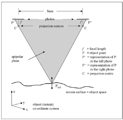
Aerial photogrammetry technology allows to measure 3D coordinates of a space and its objects (features) using 2D pictures taken from different positions. The overlapping between pictures allows to calculate 3D properties of space and features based on stereoscopy principle (Baltsavias, 1999; Eagles, 2004; Liu, 2008) as conceptualized in figure 1.2. To measure accurately ground and features elevation, a step of aerotriangulation calculation is compulsory, requiring information on picture properties regarding their position, orientation and bonding (or tie) points. The orientation on how the camera lens was pointed varies in time depending on the lens rotation due to plane or UAV roll, pitch and yaw that lead to lens rotation angles (respectively called omega, phi and kappa). The use of ground control points allows to geo-reference the dataset.
A low flight elevation, a high number of aerial pictures with different points of view and high levels of overlapping, allow to increase the accuracy and the reliability of the 3D coordinates measurement (Küng et al., 2011). Indeed, sensitivity tests on parameters photogrammetric influencing dataset quality: (i) flight altitude, (ii) image overlapping, (iii) camera pitch and (iv) weather conditions, confirmed the major influence of flight altitude on dataset quality (Leitão et al., 2015).
Figure 1.2. Stereoscopy principle in photogrammetry to get ground or object x, y, and z properties (from Linder,
2006).
In photogrammetry, the spatial resolution is the size of a pixel at the ground level. It has to be distinguished to the spectral resolution which is related to the number of spectral bands and gathered simultaneously (see Egels and Kasser, 2004). At a given spatial resolution, an object having a size three times bigger than the pixel size can be identified and interpreted.
1.1.3 Object based classification: photo-interpretation
For 3D classified dataset creation, a photo-interpretation step is necessary. Photo-interpretation allows creation of vectorial information based on photogrammetric dataset (Egels and Kasser, 2004; Linder, 2006). A photo-interpreted dataset is composed of classes of points, polylines and polygons digitalized based on photogrammetric data. Figure 1.3 illustrates the visualization of a sub-part of a photo-interpreted dataset composed of 50 classed of polylines and polygones. Important aspects in the photo-interpretation process are the classes’ definition, the photo-interpretation techniques and the dataset quality used for the photo-interpretation. These aspects will impact the design of the output classified dataset (Lu and Weng, 2007).
Figure 1.3. Visualization of elevation information of a photo-interpreted dataset gathered over an urban area
(Nice, France). Details of this specific dataset are given in chapter 2.
The step of classes’ definition has to be elaborated prior to the photo-interpretation step. The number, the nature and criteria for the definition of classes will depend on the objectives of the photo-interpretation campaign.
Photo-interpretation techniques can be made (i) automatically by algorithm use, (ii) manually by a human operator on a Digital Photogrammetric Workstation (DPW) or (iii) by a combination of the two methods. The level of accuracy is higher when the photo-interpretation is done by a human operator on a DPW, but more resources are needed as the process becomes highly time consuming (Zou et al., 2004; Lafarge, 2010). Eventually, the 3D classification of features based on photo-interpretation allows to get 3D High-Resolution topographic data over territory that offers large and adaptable perspectives for its exploitation for different purposes (Andres, 2012).
Usually, when a photo-interpreted classified dataset is provided to a user, the data is assorted with a global mean error value and with a percentage of photo-interpretation accuracy. The mean error value encompasses errors, due to material accuracy limits, to biases and to nuggets (or blunder) that compose error within the row photogrammetric data. Furthermore, a percentage of accuracy representing errors in photo-interpretation is generally provided. This percentage of accuracy represents errors in photo-interpretation
which results from feature misinterpretation addition or omission. This percentage of accuracy results from the photo-interpreted dataset comparison with field ground measurements of elevation over sub-domains of the photo-interpretation campaign (Figure 1.4). This process of control is time consuming as often based on manual operation and control, resource requiring (to gathered field measurement) and subject to operator interpretation (Andres, 2012).
Figure 1.4. Illustration of field and photo-interpreted measurement comparison that are performed to control
the level of accuracy of the photo-interpretation process.
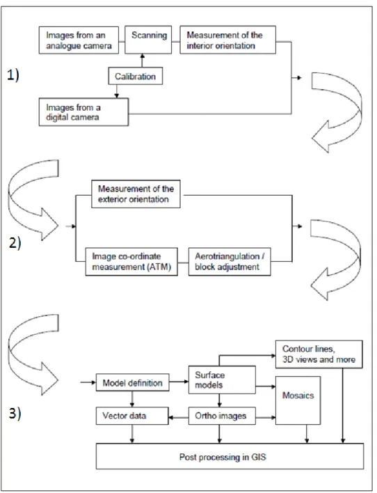
A typical workflow to illustrate the process to achieve the photo-interpretation is given in figure 1.5. With this figure, idea is not to go into details into the description of this workflow, that can vary depending on the campaigns. Nevertheless, it is interesting for a non-specialist in geomatics to understand that three loops are interconnected in this process. First, the data gathering/measurement. Impact of camera properties is the main issue here. Second, loop is the treatment of geo-referencing/calibration part. Last part of the process is the photo-interpretation part itself.
Figure 1.5. Illustration of workflow process to produce a photo-interpreted dataset as described in Linder
(2006).
It has to be mentioned that both type LiDAR and Photogrammetric topographic data gathering techniques, when mounted on aerial vectors, are not well suited to gathered underwater bathymetry. New possibilities of post-treatment of these techniques to gather river bathymetry are developing (see Feurer et al., 2008). Nevertheless, beside for really low flow condition, issues are still likely to occur due to LiDARinability to penetrate water masses (Podhoroanyi and Fedorcak, 2015) and due to visibility through water that will make photogrammetry use not relevant.
1.3
F
OCUS ON SPATIAL DISCRETIZATIONIn computing codes, the physical domain (
Ω
) can have 1, 2 or 3 dimensions in space. The discretization ofΩ
in 1D, 2D or 3D is respectively associated to variables x, y and z and called a mesh or a computational grid. The computational grid then represents the continuum where the governing partial differential equations are replaced by constructed discretized forms/solved by numerical methods (see part 2). For numerical resolution of the 2D SWEs system, the continuous variable topography information/elevation (z) is necessary for the computation, and therefore spatially discretized according to a 1D, 2D or 3D meshing process.A mesh that arises from the discretization of z within
Ω
is composed of referenced points (computational points or nodes) and of cells (or elements) that link the points together. A mesh is characterized by its dimension - 1D to 3D -, and the geometry of its cells that can be flat elements (triangles, rectangles or polygons) or elements in volume (pyramids, tetrahedron, cubes, etc.), respectively for 2D or for 3D. As recalled in Weatherill (1992), the mesh has to represent accurately the geometrical boundaries, and “gap” in the computational domain cannot occur.Main classification criteria of types of meshes are following:
If elements have identical/regular size to discretize the
Ω
, the mesh is said to be structured, whereas if the mesh is composed of elements having different sizes (but always with the same geometry) they are qualified as non-structured (Figure 1.6). In a structured mesh, all interior nodes -not located on a boundary ofΩ
- have an equal number of adjacent elements. Hybrid meshing exists,Ω
being then discretized mixing structured and non-structured sub-domains. If properties (size/shape) of elements constituting a mesh evolve with time, the mesh is referenced as Adaptive Mesh Refinment (AMR) while a mesh that has constant properties in time is referred as non-adaptive.
Parameters of a computational grid such as area or volume of the cells (resolution) and number of elements are inherent properties of the mesh. The smaller are the areas or volumes of the elements, the more the discretization gets close to the continuous variable (z), but the more the total number of elements increases. By increasing the number of cells in the mesh, the computational coast increases, not only because of the increased number of computational points in space, but also due to the temporal discretization that decreases – if
dt is adaptive in the numerical scheme - to fit with a numerical stability criterion (CFL criterion, see part 2, section 2.2.1).
Figure 1.6. Illustration of structured (left) and non-structured (right) meshing.
In 2D free surface modelling, the different types of mesh -structured, non-structured and adaptive- are used in industrial codes.
Structured computational grids, such as the commonly used Cartesian structured mesh, have the main advantages that they are often easy to use. Indeed, the DEM representing the domain can be almost straight forwardly used as a computational grid (assuming that the
DEM representing the domain is considered as already suited for the hydraulic modelling application). For practical application degradation or resampling of a HR DEM can occur due to limitations in computation resources or in data handling.
Two main disadvantages arise from the use of structured mesh. First the regular size of elements implies that the highest mesh resolution one can expect from the discretization procedure is the same over
Ω
. Hence, in areas where the physical properties of the phenomena wished to be modelled, or where the variable (elevation) does not vary, there will be an unnecessary over-discretization ofΩ
. Consequently it will involve a high computational cost along with the storage of potentially unnecessary information. Second, disadvantage of a structured Cartesian mesh is that if the flow or any singularity is orientated, in the worst case, plus or minus 45° compared to the x or y direction, the computation will artificially go through a stepwise zig-zag processing (Ma et al., 2015). As a result, the number of cells, and therefore the length over which the water will flow, is artificially increased by this process.Non-structured computational grid relies on a set of computational points that constitute the set of cells that all have the same shape (most commonly triangles in 2D), but that have variable sizes (and therefore variable areas). Most common practice is to generate first a plane mesh according to x and y directions. This process requires to give vector spatial information such as polygons, lines or points over the domain where the modeller wants the mesh to be refined. Then z values from the DEM are then applied to the mesh. Another approach, offers the possibility to direcly give criterions such as z gradient from the DEM for mesh generation and refinement.
The flexibility regarding mesh cell size, compared to structured meshes, allows to decrease the number of computational points where there is no need for accurate discretization of the variable (e.g. areas where elevation is constant) or where averaging assumptions are estimated to be fair. Automatic methods for non-structured mesh generation are reviewed in Löhner (1997) and Owens (1998). As generalized in Löhner (1997), an automatic non-structured grid generator requires:
description of the bounding surface and of the domain to be gridded;
description of elements to be generated (nature, size, shape, orientation, growing ratio criterion);
grid generation techniques.
Most commonly used grid generation techniques in 2D hydraulic non-structured mesh generation rely on, advancing front method (George and Seveno 1994), Delaunay and
constrained Delaunay triangulation methods (Weatherill, 1992), or hybrid techniques. These techniques will not be reviewed here but it is interesting to mention that a limit of these meshing algorithms is that they are not well suited for over-constrained domain mesh generation. These meshing techniques are implemented in commercial and commonly used codes mesh generator (Mike 21 mesh generator DHI (2007b)) and BlueKenue for TELEMAC CHC (2010), see conclusion of this chapter).
Adaptive Mesh Refinement (AMR) is a discretization that evolves with space and time. The aim of this type of approach is (i) to reduce computational time by optimizing number of computational points to numerical constraints related to flow properties (e.g. CFL) and (ii) to improve accuracy of the solution. Two main types of approaches are used in 2D SWEs based flood modelling.
Block-structured adaptive mesh refinement. This type of approach is a nesting of multiple levels of evolving patches of structured sub-grids that are pre-generated. Coarse grid or finer nested sub-grids are used depending on flow dynamic properties as these properties can impact numerical aspects in the solution computation. The patchwork of grids is user-chosen pre-specified refinement ratios. A modern and well-described method of AMR applied over the well documented Malpasset dam break case can be found in Georges (2011).
The other approach is a sequence of grid operations that re-generate the non-structured mesh during the computation, again depending on flow dynamic properties. Main steps in mesh regeneration are: (i) node movement, (ii) edge splitting, (iii) edge collapsing, and (iv) node movement (Tam, 2000).
1.4
F
EEBACK FORHR
TOPOGRAPHIC DATA USE IN2D
URBAN FLOODMODELLING
This first part of chapter 1 introduced the concept of HR topographic datasets and the spatial discretization processes that will influence both possibilities and accuracy of HR topographic data inclusion within flood models. As a reminder, goals of the research presented in this thesis is to develop amethod and good practices for High-Resolution (HR) topographic data use (T1) and to focus on uncertainties related to HR topographic use and inclusion in 2D flood models (T2).
Within T1 framework it is set that for the spatial extent of our applications of interest, namely urban and industrial sites HR 2D overland flow modelling, LiDAR or photogrammetry technologies settled on an aerial vector are the best suited to gathered HR topographic datasets. As enhanced in this part, qualitative difference between LiDAR and
Photogrammetric based HR datasets rely in the interpretation/classification possibilities that are more important in photogrammetry. Photo-interpreted dataset offers a broader range of possibilities for HR DEM design, in accordance with descriptions of the above-ground structure that will influence overland flow. Indeed classification of above-ground features being more extensive in photo-interpreted datasets, it will allow hydraulic modeller to design its HR DEM having a control on which elevation information should be included in it. This is especially relevant for complex environment such as urban and industrial sites, where an important diversity of above-ground elements exists. These techniques are sometimes used in a combinatory way to gather HR datasets in urban areas (Zhou et al., 2004; Abdullah et al., 2012). LiDAR and photo-interpreted datasets will be tested in our study in chapter 2. Moreover, HR topographic datasets errors have been briefly introduced in this chapter and within T2 framework, will be detailed in chapter 3 in order to compare impact of errors in HR topographic dataset and modeller choices in HR topographic data integration effects on flood modelling results.
Structured and non-structured approaches are selected as other discretization strategies (AMR) are not commonly used in practical applications. Structured and non-structured meshing processes will be tested to assess if they offer the same possibilities for HR topographic data integration within the 2D hydraulic codes (chapter 2). Idea is to compare performance of these two discretization strategies in terms of accuracy of HR urban flood models building. Moreover, ease of use and computational efficiency will be regarded as well.
Preconceived idea is that photo-interpreted dataset might be efficient for non-structured mesh generation as the data is vectorialized and should offer interesting possibilities for non-structured mesh generation. Another idea arising from the theoretical background would be the assumed advantage of non-structured grid compared to structured ones. Case study studies in chapter 2 will illustrate that these preconceived assumptions are not confirmed.
P
ART
.
2.
N
UMERICAL MODELLING OF FREE SURFACE FLOW
:
APPROXIMATING SOLUTION OF
SWE
S
2.1
F
ROMH
YPOTHESIS IN THE PHYSICAL DESCRIPTION OF THE PHENOMENATO MATHEMATICAL FORMULATION
2.1.1 From flow observation to de Saint-Venant hypothesis and
mathematical formulation
Observation of channel flow to de Saint-Venant hypothesis
In nature, examples of free surface water flow complexity are observable and numerous (e.g. flood event, runoff over urban area, etc.). In parallel there are needs for humans to use water resources and to protect themselves from flood hazard resulting from natural intense events. Engineering interest in knowing water stage and discharge along a given canal reach has conducted Barré de Saint-Venant to formulate a simplification framework from observation of flow behavior which lead to an idealistic situation or concept where flow behavior can be described and understood for practical perspectives (de Saint-Venant, 1871).
As reminded in Cunge (2012), basics behind the simplified idealistic situation is to switch from local detailed scale to a more macroscopic (several hundred meters) one. Then, at such a scale the only forces which are considered are gravity, inertial and resistance forces. Therefore, simplification introduced by de Saint-Venant are that (i) the water surface is the same over one cross section, (ii) it can be considered that flow has one privileged direction and that the flow velocity is the same over one vertical, (iii) hydrostatic pressure hypothesis and (iv) energy losses can be represented using empirical formula (Chézy like formulas). Originally, validity of this simplified framework is for a flow along an inclined channel of constant slope and cross sections.
Shallow Water Equations
Laws of mechanics can be summed up as three principles: (i) mass conservation, (ii) variation of momentum and (iii) total energy conservation. Applying above mentioned hypothesis to mechanics laws, lead to the Shallow Water Equations system (SWEs) eq. (1). Writing equations system in one dimension over a control volume included between two rectangular cross sections separated by the distance dx for a given time interval dt; we have:
(1)
where: g is the acceleration of gravity constant, h(t, x) the water depth and u(t, x) the mean flow velocity. The system of equations of Partial Differential Equations (PDEs) expressed in eq. (1) does not consider any source terms (no friction included here and no variation of topography) and is therefore called a homogeneous writing of the system. Adding source terms eq. (2), the SWEs is called non-homogeneous system and writes as follow in 2D:
(2)
where, the unknowns are the velocities vector components u(x, y, t), v(x, y, t) [m/s] and the water height h(x, y, t). The subscript x (respectively y) stands for the x-direction (respectively y-direction). and are the ground slopes and Sfx and Sfy are the friction terms. Component I of the momentum equations is the time evolution, II is the convection term, III is the hydrostatic pressure, IV is the transversal component (in 2D only) and the source term V includes the slope and the energy loses related to resistance (friction) against channel boundaries.
Analytical solutions of this system of equations exist only for a few theoretical cases where initial and boundary conditions are known (e.g. SWASHES library compiling a couple of 1D and 2D theoretical cases, see (Delestre et al., 2013)) or in case of backwater curve occurrences. Nevertheless for cases of flood event which are of prime interest for practitioners, no general analytical solution exists. Indeed, the perfect knowledge of information of initial and boundary conditions can only be assumed or approached in applied natural cases. Therefore, from a mathematical point of view, the exact solution of this system cannot be obtained in such a context. Consequently, the exact solution can only be approximated with a numerical method.
As it will be explained in section 1.2, the numerical resolution of SWEs system can be computationally resource demanding. Simplified versions of the SWEs system exist and are made from simplifying hypothesis regarding terms in the momentum equation of the SWEs system. Most commonly used approximate models are the kinematic waves, where the momentum equation (from eq. (2)) is reduced to the expression of the term V, and the