An Algebraic Method for Compressing Very Large Symbolic Data Tables

RESEARCH OUTPUTS / RÉSULTATS DE RECHERCHE

Author(s) - Auteur(s) :

Publication date - Date de publication :

Permanent link - Permalien :

Rights / License - Licence de droit d’auteur :

Institutional Repository - Research Portal

Dépôt Institutionnel - Portail de la Recherche

researchportal.unamur.be

University of Namur

An Algebraic Method for Compressing Very Large Symbolic Data Tables

Tzitzikas, Yannis

Proceedings of the Workshop on Symbolic and Spatial Data Analysis (SSDA) of ECML/PKDD 2004

Publication date: 2004

Link to publication

Citation for pulished version (HARVARD):

Tzitzikas, Y 2004, An Algebraic Method for Compressing Very Large Symbolic Data Tables. in Proceedings of the Workshop on Symbolic and Spatial Data Analysis (SSDA) of ECML/PKDD 2004.

General rights

Copyright and moral rights for the publications made accessible in the public portal are retained by the authors and/or other copyright owners and it is a condition of accessing publications that users recognise and abide by the legal requirements associated with these rights. • Users may download and print one copy of any publication from the public portal for the purpose of private study or research. • You may not further distribute the material or use it for any profit-making activity or commercial gain

• You may freely distribute the URL identifying the publication in the public portal ?

Take down policy

If you believe that this document breaches copyright please contact us providing details, and we will remove access to the work immediately and investigate your claim.

Workshop on Symbolic and Spatial Data Analysis (SSDA’2004) of ECML/PKDD 2004, Pisa, Italy, September 2004

An Algebraic Method for Compressing Very

Large Symbolic Data Tables

Yannis Tzitzikas

Institut d’Informatique F.U.N.D.P. (University of Namur) Rue Grandgagnage 21, B-5000, Belgium

Email : [email protected]

Abstract. Although symbolic data tables summarize huge sets of data they can still become very large in size. This paper proposes a method for compressing a symbolic data table using the recently emerged Compound Term Composition Algebra. One charisma of CTCA is that the closed world hypotheses of its operations can lead to a remarkably high ”compression ratio”. The compacted form apart from having much lower storage space requirements, it allows designing more efficient algorithms for symbolic data analysis.

1

Introduction

As recent surveys state1_{, the world produces between 1 and 2 exabytes (2}60_bytes)

of unique information per year, 90% of which is digital and with a 50% annual growth rate. Undoubtedly, this is a boon rather than a anathema. In addition, this plethoric growth rate has stimulated the development of new techniques and automated tools for assisting the transformation of large amounts of data into useful information and knowledge (see data mining and knowledge discovery in databases). Symbolic data analysis [3, 4] has been introduced in order to solve the problem of the analysis of data that are given on an aggregated form, i.e. where quantitative variables are given by intervals and where categorical variables are given by histograms. This kind of data are generated when we summarize huge sets of data. Inescapably, even a symbolic data table could become very large in size, making its management problematic in terms of both storage space and computational time.

This paper aims to convey some recent advances from the area of knowledge representation (in particular from the area of faceted taxonomies and faceted classification), that could be exploited for symbolic data analysis. Specifically, this paper gives the theoretical foundation of a novel method that can be used to

compress (i.e. to reduce the storage space requirements) of large symbolic data

tables. The proposed compression is lossless i.e. from the compressed form we can infer exactly what we can from the original symbolic data table.

The contribution of the method is not exhausted to storage space minimiza-tion as the resulting compact form could allow the design more efficient symbolic analysis algorithms.

For reasons of space, this paper describes only the principles of this method and gives some indicative examples. The interested reader is referred to the references that are given. The rest of this paper is organized as follows. Section 2 sketches the idea and Section 3 recalls the basics of the Compound Term

Composition Algebra (CTCA), upon which the proposed method is founded.

Subsequently, Section 4 describes in more detail the steps of this technique and Section 5 gives some indicative examples of compression using CTCA. Finally, Section 6 concludes the paper and identifies issues for further research.

2

The Idea

A Symbolic data table is a table of data where the columns are the symbolic

variables which are used in order to describe a set of units called individuals.

Rows are called symbolic descriptions of these individuals because they are not as usual, only tuples of single quantitative or categorical values. For instance, the values of the cells can be intervals (if the variable is quantitative) or frequency distributions (if the variable is categorical). Recall that in classical data analysis a cell can have a single quantitative or categorical value. In general, we could distinguish variables according to their range to (a) single quantitative (e.g. age=18), (b) single categorical (or taxonomic) (e.g. color=red), (c) multi-valued quantitative or categorical (e.g. age={11, 18}, color={red, green}) (d) interval (e.g. age=[10,20]), and (e) multi-valued with weights (e.g. histograms). Clearly, (a) and (b) are special cases of (c), while (c) is special case of (e) (i.e. when all weights are either 0 or 1) for more see [4].

This paper proposes a method for compacting a symbolic data table by ex-ploiting the Compound Term Composition Algebra (CT CA). CTCA is a recently emerged algebra that allows specifying the valid (meaningful) compound terms (conjunction of terms) over a faceted taxonomy in a flexible and efficient manner (for more see [13, 12]). A system around CTCA has already been developed (FAS-TAXON [14]) and there has already been proposed a Web annotation language that allows exchanging faceted taxonomies and expressions of CTCA (for more see XFML+CAMEL [2]). In brief, a faceted taxonomy is a set of taxonomies each one describing the domain of interest from a different (preferably orthogonal) point of view (for more about faceted classification and analysis see [10, 5, 15, 6, 7]). Faceted taxonomies are used in Web Catalogs, Libraries [7], Software Repos-itories [8, 9], and several others application domains. Current interest in faceted taxonomies is also indicated by several recent or ongoing projects (like FATKS2_,

FACET3_{, FLAMENGO}4_{) and the emergence of XFML [1](Core-eXchangeable}

Faceted Metadata Language) a markup language for applying the faceted clas-sification paradigm on the Web. Having a faceted taxonomy each domain object (e.g. book or Web page) can be indexed using a compound term, i.e., a set of terms containing one or more terms from each facet. We shall use the term

mate-rialized faceted taxonomy to refer to a faceted taxonomy accompanied by a set of

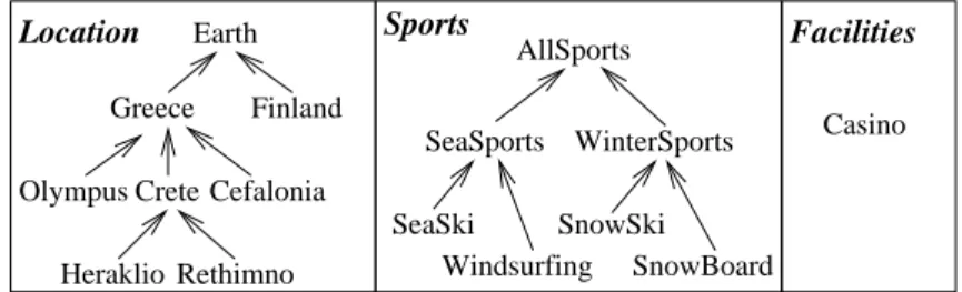
object indices. For example, Figure 1 shows a very small but indicative faceted taxonomy consisting of three facets that is appropriate for indexing hotel Web pages. SeaSports WinterSports AllSports SnowBoard SeaSki Casino Greece Heraklio Rethimno Crete Finland Earth Olympus Sports _Facilities Cefalonia Windsurfing SnowSki Location

Fig. 1. A faceted taxonomy for indexing hotel Web pages

Roughly, and according to the above perspective and phraseology, each sym-bolic data table can be viewed as a materialized faceted taxonomy. This analogy is not hard to grasp. Each symbolic variable can be viewed as a facet. Now the range of each symbolic variable can be viewed as a taxonomy, i.e. as a partially ordered set of terms (clearly, categories, intervals, and subsets are partially or-dered domains). Now each row of the symbolic data table can be viewed as an

object that has been indexed according to a faceted taxonomy, i.e. as an object

that has been associated with a compound term of the faceted taxonomy, i.e. with a set of values from the range of the symbolic variables.

Several algorithms for finding an expression of CTCA that describes those compound terms that are extensionally valid in a materialized faceted taxonomy were given and analyzed in [11]. In other words, these algorithms mine an ex-pression of CTCA that specifies the set of all distinct compound terms that are meaningful, where a compound term is considered meaningful if it is applicable to at least one object of the object base. It follows, that the same algorithms can be exploited for the problem at hand, specifically for finding a short (in storage space) expression of CTCA that specifies the rows of a symbolic data table.

Specifically, this paper focuses on symbolic variables with partially ordered ranges, i.e. taxonomically-ordered categorical, multi-valued quantitative or cat-egorical, and interval-valued variables. The reason is that in this case the em-ployment of CTCA yields remarkably high compression ratios. However, CTCA can be applied even on unordered ranges, i.e. on sets (we can view a set as a

3 _{http://www.glam.ac.uk/soc/research/hypermedia/facet proj/index.php} 4 _{http://bailando.sims.berkeley.edu/flamenco.html}

poset with an empty ordering relation), so the proposed method can be also applied on variables whose range is a set of histograms. However, an issue for further research is to investigate ordering relations over histograms because their availability would allow obtaining higher compression ratios even for this kind of variables (especially when lossy compression is tolerable).

3

Faceted Taxonomies and the Compound Term

Composition Algebra

Table 1 below recalls in brief the basic notions around taxonomies, faceted tax-onomies and materialized faceted taxtax-onomies (for more please refer to [13]).

Name Notation Definition

terminology T a set of names called terms

subsumption ≤ a preorder relation (reflexive and transitive)

taxonomy (T , ≤) T is a terminology, ≤ a subsumption relation over T faceted taxonomy F= {F1, ..., Fk} Fi= (Ti, ≤i), for i = 1, ..., k and all Tiare disjoint compound term over T s any subset of T (i.e. any element of P(T ))

compound terminology S a subset of P(T ) that includes ∅

compound ordering ¹ s ¹ s0 _{iff ∀t}0_{∈ s}0 _{∃t ∈ s such that t ≤ t}0_.

broaders of s Br(s) {s0_{∈ P (T ) | s ¹ s}0_}

narrowers of s Nr(s) {s0_{∈ P (T ) | s}0_{¹ s}}

broaders of S Br(S) ∪{Br(s) | s ∈ S}

narrowers of S N r(S) ∪{Nr(s) | s ∈ S}

object domain Obj any denumerable set of objects

interpretation of T I any function I : T → 2Obj

model of (T , ≤)

induced by I I¯ I(t) = ∪{I(t¯ 0_{) | t}0_{≤ t}}

materialized (F, I) F is a faceted taxonomy {F1, ..., Fk}, faceted taxonomy I is an interpretation of T =Si=1,kTi

Table 1. Notations

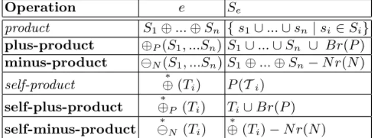
CTCA was proposed for defining the meaningful compound terms over a faceted taxonomy in a flexible and efficient manner. The problem of meaning-less compound terms and the effort needed to specify the meaningful ones is a practical problem identified even by Ranganatham himself [10] (80 years ago) and it is probably the main reason why faceted taxonomies have not dominated every application domain despite their uncontested advantages over the single-hierarchical taxonomies. CTCA is the only well-founded and flexible solution to this problem.

CTCA has four basic algebraic operations, namely, plus-product (⊕),

operations over P(T ), the powerset of T , where T is the union of the terminolo-gies of all facets. The initial operands, thus the building blocks of the algebra, are the basic compound terminologies, which are the facet terminologies with the only difference that each term (for reasons of notational simplicity) is viewed a singleton. Specifically, the basic compound terminology of a terminology Ti is

defined as: Ti= {{t} | t ∈ Ti}∪{∅}. If e is an expression, Sedenotes the outcome

of this expression and is called the compound terminology of e. An expression e over F is defined according to the following grammar (i = 1, ..., k):

e ::= ⊕P(e, ..., e) | ªN (e, ..., e) | ∗

⊕P Ti | ∗

ªN Ti| Ti,

where the parameters P and N denote sets of valid and invalid compound terms over the range of the operation, respectively. Roughly, CTCA allows specifying the valid compound terms over a faceted taxonomy by providing a small set of valid (P ) and a small set of invalid (N ) compound terms. The self-product op-erations allow specifying the meaningful compound terms over one facet. Specif-ically, the definition of each operation of CTCA is summarized in Table 2 where

S, S0_{denote compound terminologies. In addition, (S}

e, ¹) is called the compound

taxonomy of e. The associated inference mechanism and the closed world

assump-tion of each operaassump-tion, makes the task of specifying the meaningful compound terms flexible and fast. The algorithm given in [13] takes as input a expression e and a compound term s, and checks whether s ∈ Se. This algorithm has

polyno-mial time complexity, specifically O(|T |3_{∗ |P ∪ N |), where P denotes the union}

of all P parameters and N denotes the union of all N parameters appearing in

e. Operation e Se product S1⊕ ... ⊕ Sn { s1∪ ... ∪ sn| si∈ Si} plus-product ⊕P(S1, ...Sn) S1∪ ... ∪ Sn ∪ Br(P ) minus-product ªN(S1, ...Sn) S1⊕ ... ⊕ Sn− N r(N ) self-product ⊕ (T∗ i) P (Ti) self-plus-product ⊕∗P (Ti) Ti∪ Br(P ) self-minus-product ª∗N(Ti) ∗ ⊕ (Ti) − N r(N )

Table 2. The operations of the Compound Term Composition Algebra

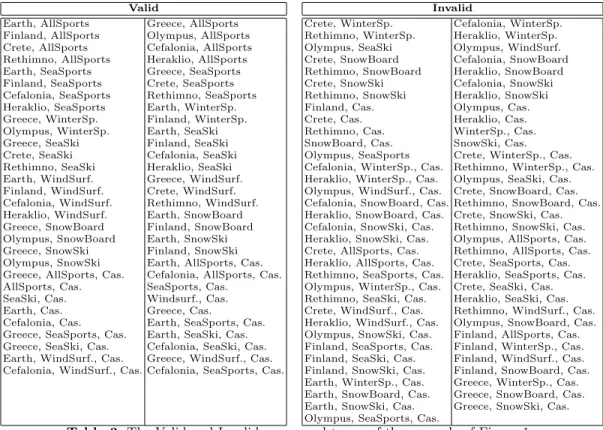
For example, Table 3 (that is found on the appendix) shows the partition of the compound terms of the faceted taxonomy of Figure 1 into the set of valid and the set of invalid compound terms. Instead of defining this partition explicitly, with CTCA one can define it in a more flexible and quick manner. Specifically, this partition can be specified by the subsequent expression:

e = (Location ªN Sports) ⊕PF acilities

with the following P and N parameters:

{Cef alonia, W interSports}} P = {{Cef alonia, SeaSki, Casino},

{Cef alonia, W indsurf ing, Casino}}

CTCA can be exploited both forthrightly and reversely, i.e. a designer can formulate an expression in order to specify quickly the desired set of compound terms, while from an existing set of compound terms an algorithm can find an expression that describes these compound terms. It is the latter direction that is appropriate for symbolic data analysis.

In order to apply CTCA for compacting symbolic data tables we only have to consider facets that range a set of intervals. This is rather a trivial extension, as we can consider each interval [a,b] as a term. The ordering between interval terms can be inferred easily, i.e. [a, b] ≤ [c, d] iff c ≤ a and b ≤ d, and there is no need for storing these relationships. So CTCA applies on intervals as it is.

Note that the disjointness of facet terminologies can be implemented in prac-tise by prefixing each value of the range of a variable by the variable name.

4

The Technique

Roughly, a symbolic data table with k columns and n rows can be compressed in three steps:

(a) At first, we organize the range of each variable as a partially ordered set (poset) and we store it.

Note that if the range of a variable is a set of categories that are partially ordered, i.e. a taxonomy, then it is enough to store only the transitive reduc-tion of the taxonomic ordering. If the range of a variable is a set R of subsets of a set D (i.e. R ⊆ P(D) where P(D) denotes the powerset of D), then we again have a poset, i.e. the partially ordered set (R, ⊆). In this case we only have to store R as here the ordering relation corresponds to the relation ⊆ which can be deduced algorithmically (for any two sets s and s0_{we can check}

whether s ⊆ s0_{). Finally, if the range of a variable is a set of intervals L then}

we only have to store L because again the ordering relation can be deduced. (b) Subsequently, we can run one of the algorithms described in [11] that mine

an expression of CTCA that describes exactly the rows of our table. Using the notations of the previous section, the objective of these algorithms is to find an expression e such that

Se= {s ∈ P(T ) | ¯I(s) 6= ∅}

where if s = {t1, ..., tk} then I(s) = I(t1) ∩ ... ∩ I(tk). That paper gives the

algorithms for two straightforward methods for extracting a plus-product and a minus-product expression and an exhaustive algorithm for finding the

shortest (i.e. the most space economical) expression. The latter yields

closed-world assumptions of CTCA, but its computational complexity if re-markably higher. For reasons of space the description of the algorithms is omitted.

(c) Finally, we store the mined expression and its parameters (e.g. in a relational database as it has been done in FASTAXON [14]).

After the above process we can delete the symbolic data table and keep stored only the posets and the mined expression e. Now suppose that we want to check whether an arbitrary tuple s (over the domain of our variables) exists in the table. We don’t have to restore the initial table in order to answer this question. Instead, we run the algorithm described in [13] which takes as input a faceted taxonomy, an expression e and a compound term s and decides in polynomial time whether s ∈ Se.

Another remark that should be mentioned here is that it is also possible to

browse the symbolic table without having to reconstruct it. Specifically, by the

faceted taxonomy F and the expression e we can derive dynamically a navigation tree that allows browsing all compound terms in Seusing the algorithm described

in [13] that has been implemented in FASTAXON [14].

Of course, at any time we could run a (quite simple) algorithm for recon-structing the symbolic data table at its original form.

5

Indicative Examples

This section presents a small number of intuitive examples for demonstrating the potential of CTCA for the problem at hand.

Consider that we have two variables A and B. The variable A ranges over the set {a1, a2, a3} and assume that this set is ordered according to a taxonomic

relation (subsumption) as follows: a3 ≤ a2 ≤ a1. Now consider the following

table

A B

a1b1

a2b1

a3b1

The rows of this table can be described by the expression e = A ⊕PB where

P = {{a3, b1}}. One can easily see that Se= {{a1, b1}, {a2, b1}, {a3, b1}}.

Alternatively, they can be described by the expression e0 _{= A ª}

N B where

N = ∅ as A ª∅B = A ⊕ B = {{a1, b1}, {a2, b1}, {a3, b1}}.

Now assume that the range of A is the taxonomy ({a1, a2, a3, a4}, {a2 ≤

a1, a3≤ a2, a4≤ a2}), the range of B is the taxonomy ({b1, b2}, {b2≤ b1}) and

A B {a3, a4} b1 a2 b2 a1 b1 a1 b2 a2 b1 a3 b1

Here and in order to describe the set {a3, a4} we are obliged to use a self-product

operation over A. We can describe the rows of this table by any of the above three expressions:

– e1= (

∗

⊕P 1(A)) ⊕P 2(B) where P 1 = {{a3, a4}} and P 2 = {{a3, a4, b1}, {a2, b2}}

– e2= (

∗

ªN 1(A)) ⊕P 2(B) where N 1 = ∅ and P 2 = {{a3, a4, b1}, {a2, b2}}.

– e3= (

∗

ªN 1(A)) ªN 2(B) where N 1 = ∅ and N 2 = {{a3, a4, b2}}.

Clearly, e3 is the most space economical expression as it requires us to keep

stored only one compound term that consists of three single terms. Example 1.

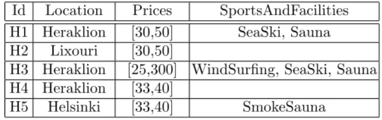
Assume that we have the following table with information about hotels:

Id Location Prices H1 Heraklion [30,50] H2 Lixouri [33,40] H3 Heraklion [25,300] H4 Heraklion [33,40]

For notational simplicity we shall use A for Location and B for Prices. The above table (by ignoring the first column) can be represented by the expression

e1= AªN1B where N1= ∅ as all combinations between the domain of these two

variables are valid (appear or are semantically inferred from those that appear). Specifically, although Lixouri does not co-appear in the table with neither [30,50] nor with [25, 300], these combination are valid because since there is a hotel at Lixouri with rates [33,40], it is true that we can find a hotel at Lixouri at [30,50] or [25,300] Euros.

Example 2.

Let us now modify one cell of the above table:

Id Location Prices H1 Heraklion [30,50] H2 Lixouri [30,50] H3 Heraklion [25,300] H4 Heraklion [33,40]

This table can be represented by the expression e2 = A ªN2 B where N2 =

{{Lixouri, [33, 40]}}.

Example 3.

Let us now add one more row and one more column to the table of the previous example

Id Location Prices SportsAndFacilities H1 Heraklion [30,50] SeaSki, Sauna H2 Lixouri [30,50]

H3 Heraklion [25,300] WindSurfing, SeaSki, Sauna H4 Heraklion [33,40]

H5 Helsinki [33,40] SmokeSauna

Let C denote the variable SportsAndFacilities and let the range of C be or-ganized as shown in Figure 2. Let’s now try finding the expression that describes this table. The ”subtable” that consists of the columns B and C is described by the expression e2as we saw earlier in Example 2. Now the range of variable C can

be expressed using a self-product operation, specifically by eC= ∗

⊕PC (C) where

PC= {{W indSurf ing, SeaSki, Sauna}}. Note that if SmokeSauna did not

be-long to the range of C then we would have defined eC as follows: eC= ∗

ªNC (C)

with NC= ∅.

In order to represent the whole table we have to combine e2 and eC. This

can be obtained as: e3= e2⊕P3eC where

P3= {{Heraklion, [25, 300], Lixouri, {W indSurf ing, SeaSki, Sauna}}

Windsurfing SeaSports SeaSki SportsAndFacilities Sauna SmokeSauna

Fig. 2. The range of the symbolic variable SportsAndFacilities

Summarizing, CTCA can indeed compact a symbolic data table and can yield to remarkably high compression ratios. One can easily guess that the more sym-bolic variables we have and the more numerous are the ranges of these variables, the higher compression ratio we can achieve with CTCA.

6

Epilogue

Although symbolic data tables summarize huge sets of data they can still become very large in size. This paper proposes a method for compressing a symbolic

data table using the recently emerged Compound Term Composition Algebra (CTCA). One charisma of CTCA for the problem at hand is that the closed world hypotheses of its operations (described analytically at [12]) can lead to a remarkably high ”compression ratio”. Another remark that have to be mentioned here is that the functionality offered by CTCA cannot be obtained by using a classical logic-based formalism, like Description Logics, as it was shown in [12]. At last, but not least, this paper identified the analogies between symbolic data tables and faceted taxonomies (and CTCA) in order to act as a two-way canal between the two communities. An issue for further research is the characteriza-tion of the proposed approach according to Kolmogorov’s complexity and the extension of this method for frequency-valued symbolic variables.

Acknowledgement

Many thanks to Tonia Dellaporta for the fruitful discussions on this issue and to Monique Noirhomme-Fraiture for providing me with very useful material for Symbolic Data Analysis.

References

1. “XFML: eXchangeable Faceted Metadata Language”. http://www.xfml.org. 2. “XFML+CAMEL:Compound term composition Algebraically-Motivated

Expres-sion Language”. http://www.csi.forth.gr/markup/xfml+camel.

3. H. H. Bock and E. Diday. Analysis of Symbolic Data. Springer-Verlag, 2000. ISBN: 3-540-66619-2.

4. Edwin Diday. “An Introduction to Symbolic Data Analysis and the Sodas Soft-ware”. Journal of Symbolic Data Analysis, 0(0), 2002. ISSN 1723-5081.

5. Elizabeth B. Duncan. “A Faceted Approach to Hypertext”. In Ray McAleese, editor, HYPERTEXT: theory into practice, BSP, pages 157–163, 1989.

6. P. H. Lindsay and D. A. Norman. Human Information Processing. Academic press, New York, 1977.

7. Amanda Maple. ”Faceted Access: A Review of the Literature”, 1995. http://theme.music.indiana.edu/tech s/mla/facacc.rev.

8. Ruben Prieto-Diaz. “Classification of Reusable Modules”. In Software Reusability.

Volume I, chapter 4, pages 99–123. acm press, 1989.

9. Ruben Prieto-Diaz. “Implementing Faceted Classification for Software Reuse”.

Communications of the ACM, 34(5):88–97, 1991.

10. S. R. Ranganathan. “The Colon Classification”. In Susan Artandi, editor, Vol IV

of the Rutgers Series on Systems for the Intellectual Organization of Information.

New Brunswick, NJ: Graduate School of Library Science, Rutgers University, 1965. 11. Yannis Tzitzikas and Anastasia Analyti. “Mining the Meaningful Compound Terms from Materialized Faceted Taxonomies ”, 2004. (Submitted for publica-tion in Knowledge and Informapublica-tion Systems Journal).

12. Yannis Tzitzikas, Anastasia Analyti, and Nicolas Spyratos. “The Semantics of the Compound Terms Composition Algebra”. In Procs. of the 2nd Intern. Conference

on Ontologies, Databases and Applications of Semantics, ODBASE’2003, pages

13. Yannis Tzitzikas, Anastasia Analyti, Nicolas Spyratos, and Panos Constantopou-los. “An Algebraic Approach for Specifying Compound Terms in Faceted Tax-onomies”. In Information Modelling and Knowledge Bases XV, 13th

European-Japanese Conference on Information Modelling and Knowledge Bases, EJC’03,

pages 67–87. IOS Press, 2004.

14. Yannis Tzitzikas, Raimo Launonen, Mika Hakkarainen, Pekka Kohonen, Tero Lep-panen, Esko SimLep-panen, Hannu Tornroos, Pekka Uusitalo, and Pentti Vanska. “FAS-TAXON: A system for FAST (and Faceted) TAXONomy design.”. In Proceedings

of 23th Int. Conf. on Conceptual Modeling, ER’2004, Shanghai, China, November

2004. (an on-line demo is available at http://fastaxon.erve.vtt.fi/).

15. B. C. Vickery. “Knowledge Representation: A Brief Review”. Journal of

Docu-mentation, 42(3):145–159, 1986.

Valid

Earth, AllSports Greece, AllSports Finland, AllSports Olympus, AllSports Crete, AllSports Cefalonia, AllSports Rethimno, AllSports Heraklio, AllSports Earth, SeaSports Greece, SeaSports Finland, SeaSports Crete, SeaSports Cefalonia, SeaSports Rethimno, SeaSports Heraklio, SeaSports Earth, WinterSp. Greece, WinterSp. Finland, WinterSp. Olympus, WinterSp. Earth, SeaSki Greece, SeaSki Finland, SeaSki Crete, SeaSki Cefalonia, SeaSki Rethimno, SeaSki Heraklio, SeaSki Earth, WindSurf. Greece, WindSurf. Finland, WindSurf. Crete, WindSurf. Cefalonia, WindSurf. Rethimno, WindSurf. Heraklio, WindSurf. Earth, SnowBoard Greece, SnowBoard Finland, SnowBoard Olympus, SnowBoard Earth, SnowSki Greece, SnowSki Finland, SnowSki Olympus, SnowSki Earth, AllSports, Cas. Greece, AllSports, Cas. Cefalonia, AllSports, Cas. AllSports, Cas. SeaSports, Cas.

SeaSki, Cas. Windsurf., Cas. Earth, Cas. Greece, Cas.

Cefalonia, Cas. Earth, SeaSports, Cas. Greece, SeaSports, Cas. Earth, SeaSki, Cas. Greece, SeaSki, Cas. Cefalonia, SeaSki, Cas. Earth, WindSurf., Cas. Greece, WindSurf., Cas. Cefalonia, WindSurf., Cas. Cefalonia, SeaSports, Cas.

Invalid

Crete, WinterSp. Cefalonia, WinterSp. Rethimno, WinterSp. Heraklio, WinterSp. Olympus, SeaSki Olympus, WindSurf. Crete, SnowBoard Cefalonia, SnowBoard Rethimno, SnowBoard Heraklio, SnowBoard Crete, SnowSki Cefalonia, SnowSki Rethimno, SnowSki Heraklio, SnowSki Finland, Cas. Olympus, Cas. Crete, Cas. Heraklio, Cas. Rethimno, Cas. WinterSp., Cas. SnowBoard, Cas. SnowSki, Cas. Olympus, SeaSports Crete, WinterSp., Cas. Cefalonia, WinterSp., Cas. Rethimno, WinterSp., Cas. Heraklio, WinterSp., Cas. Olympus, SeaSki, Cas. Olympus, WindSurf., Cas. Crete, SnowBoard, Cas. Cefalonia, SnowBoard, Cas. Rethimno, SnowBoard, Cas. Heraklio, SnowBoard, Cas. Crete, SnowSki, Cas. Cefalonia, SnowSki, Cas. Rethimno, SnowSki, Cas. Heraklio, SnowSki, Cas. Olympus, AllSports, Cas. Crete, AllSports, Cas. Rethimno, AllSports, Cas. Heraklio, AllSports, Cas. Crete, SeaSports, Cas. Rethimno, SeaSports, Cas. Heraklio, SeaSports, Cas. Olympus, WinterSp., Cas. Crete, SeaSki, Cas. Rethimno, SeaSki, Cas. Heraklio, SeaSki, Cas. Crete, WindSurf., Cas. Rethimno, WindSurf., Cas. Heraklio, WindSurf., Cas. Olympus, SnowBoard, Cas. Olympus, SnowSki, Cas. Finland, AllSports, Cas. Finland, SeaSports, Cas. Finland, WinterSp., Cas. Finland, SeaSki, Cas. Finland, WindSurf., Cas. Finland, SnowSki, Cas. Finland, SnowBoard, Cas. Earth, WinterSp., Cas. Greece, WinterSp., Cas. Earth, SnowBoard, Cas. Greece, SnowBoard, Cas. Earth, SnowSki, Cas. Greece, SnowSki, Cas. Olympus, SeaSports, Cas.

Table 3. The Valid and Invalid compound terms of the example of Figure 1 As the facet Location has 8 terms, the facet Sports has 7 terms, and the facet F acilities has one term, the number of compound terms that contain at most 1 term from each facet is 9*8*2 = 144. This table contains 60 valid and 67 invalid compound terms, thus 127 in total. By adding the (8+7+1=16) singletons (which were omitted from the column of valid) and the empty set we reach the 144.