Multilevel model reduction for uncertainty quantification in computational structural dynamics

HAL Id: tel-01417686

https://tel.archives-ouvertes.fr/tel-01417686

Submitted on 15 Dec 2016

HAL is a multi-disciplinary open access

archive for the deposit and dissemination of sci-entific research documents, whether they are pub-lished or not. The documents may come from teaching and research institutions in France or abroad, or from public or private research centers.

L’archive ouverte pluridisciplinaire HAL, est destinée au dépôt et à la diffusion de documents scientifiques de niveau recherche, publiés ou non, émanant des établissements d’enseignement et de recherche français ou étrangers, des laboratoires publics ou privés.

quantification in computational structural dynamics

Olivier Ezvan

To cite this version:

Olivier Ezvan. Multilevel model reduction for uncertainty quantification in computational structural dynamics. Mechanics [physics.med-ph]. Université Paris Est, 2016. English. �tel-01417686�

UNIVERSITE PARIS-EST

Ann´

ee 2016

TH`

ESE

pour obtenir le grade de

DOCTEUR DE L’UNIVERSIT´

E PARIS-EST

Discipline: M´

ecanique

pr´

esent´

ee et soutenue publiquement

par

Olivier Ezvan

le 23 septembre 2016

Titre:

Multilevel model reduction for uncertainty quantification

in computational structural dynamics

JURY

M. Louis J´EZ´EQUEL, Professeur, ECL, pr´esident

M. Geert DEGRANDE, Professeur, KU Leuven, rapporteur

M. Jean-Fran¸cois DE ¨U, Professeur, CNAM, rapporteur

M. Christian SOIZE, Professeur, UPEM, directeur de th`ese

M. Anas BATOU, Maˆıtre de Conf´erences, UPEM, co-encadrant

Acknowledgments

Je remercie les professeurs G. Degrande et J.-F. De¨u de m’avoir fait l’honneur de

rapporter ma th`ese. J’ai ´et´e tr`es sensible `a leurs rapports de pr´e-soutenance, riches

de conseils et d’enthousiasme. Je remercie le professeur L. J´ez´equel d’avoir assur´e

le rˆole de pr´esident du jury ainsi que L. Gagliardini d’avoir examin´e ma th`ese.

Pour leur temps `a tous, consacr´e `a l’´etude de mes travaux, et pour l’ensemble de

leurs questions et remarques lors de la soutenance, ayant permis un ´echange tr`es

enrichissant et fructueux, j’en suis `a la fois honor´e et reconnaissant.

Mes remerciements vont maintenant bien-sˆur au professeur C. Soize, mon

di-recteur de th`ese, qui m’a offert un cadre de travail id´eal `a tout point de vue. Je le

remercie plus particuli`erement pour son investissement des plus g´en´ereux pour me

guider tout au long de cette th`ese. Je remercie ´egalement mon co-encadrant de

th`ese, A. Batou, pour son implication soutenue et son aide tr`es ´etroite, lesquelles

contribuant `a mon sentiment d’avoir profit´e d’un encadrement exceptionnel.

Je me dois ´egalement de remercier l’ensemble des membres du laboratoire MSME

pour leur gentillesse et sympathie, de leur soutien notamment lors des congr`es, ou

encore de leurs enseignements dont j’ai pu b´en´eficier avant et pendant ma th`ese.

Sans oublier les non-permanents de MSME, pour la plupart doctorants, pour ces bons moments et pour leur soutien.

Il va sans dire que je suis redevable du soutien inconditionnel et atemporel de ma

iii

Summary

This work deals with an extension of the classical construction of reduced-order models (ROMs) that are obtained through modal analysis in computational linear structural dynamics. It is based on a multilevel projection strategy and devoted to complex structures with uncertainties. Nowadays, it is well recognized that the predictions in structural dynamics over a broad frequency band by using a finite element model must be improved in taking into account the model uncertainties induced by the modeling errors, for which the role increases with the frequency. In such a framework, the nonparametric probabilistic approach of uncertainties is used, which requires the introduction of a ROM. Consequently, these two aspects, frequency-evolution of the uncertainties and reduced-order modeling, lead us to consider the development of a multilevel ROM in computational structural dy-namics, which has the capability to adapt the level of uncertainties to each part of the frequency band. In this thesis, we are interested in the dynamical analysis of complex structures in a broad frequency band. By complex structure is intended a structure with complex geometry, constituted of heterogeneous materials and more specifically, characterized by the presence of several structural levels, for instance, a structure that is made up of a stiff main part embedding various flex-ible sub-parts. For such structures, it is possflex-ible having, in addition to the usual global-displacements elastic modes associated with the stiff skeleton, the appari-tion of numerous local elastic modes, which correspond to predominant vibraappari-tions of the flexible parts. For such complex structures, the modal density may sub-stantially increase as soon as low frequencies, leading to high-dimension ROMs with the modal analysis method (with potentially thousands of elastic modes in low frequencies). In addition, such ROMs may suffer from a lack of robustness with respect to uncertainty, because of the presence of the numerous local dis-placements, which are known to be very sensitive to uncertainties. It should be noted that in contrast to the usual long-wavelength global displacements of the low-frequency (LF) band, the local displacements associated with the struc-tural sub-levels, which can then also appear in the LF band, are characterized by short wavelengths, similarly to high-frequency (HF) displacements. As a result, for the complex structures considered, there is an overlap of the three vibration regimes, LF, MF, and HF, and numerous local elastic modes are intertwined with the usual global elastic modes. This implies two major difficulties, pertaining to uncertainty quantification and to computational efficiency. The objective of this thesis is thus double. First, to provide a multilevel stochastic ROM that is able to take into account the heterogeneous variability introduced by the overlap of the three vibration regimes. Second, to provide a predictive ROM whose dimension

is decreased with respect to the classical ROM of the modal analysis method. A general method is presented for the construction of a multilevel ROM, based on three orthogonal reduced-order bases (ROBs) whose displacements are either LF-, MF-, or HF-type displacements (associated with the overlapping LF, MF, and HF vibration regimes). The construction of these ROBs relies on a filtering strategy that is based on the introduction of global shape functions for the kinetic energy (in contrast to the local shape functions of the finite elements). Implementing the nonparametric probabilistic approach in the multilevel ROM allows each type of displacements to be affected by a particular level of uncertainties. The method is applied to a car, for which the multilevel stochastic ROM is identified with respect to experiments, solving a statistical inverse problem. The proposed ROM allows for obtaining a decreased dimension as well as an improved prediction with respect to a classical stochastic ROM.

Short summary

For some complex dynamical structures exhibiting several structural scales, nu-merous local displacements can be intertwined with the usual global displace-ments, inducing an overlap of the low-, medium-, and high-frequency vibration regimes (LF, MF, HF). Hence the introduction of a multilevel reduced-order model (ROM), based on three reduced-order bases (ROBs) that are constituted of either LF-, MF-, or HF-type displacements. These ROBs are obtained using a filtering method based on global shape functions for the kinetic energy. First, thanks to the filtering of local displacements, the dimension of the multilevel ROM is reduced compared to classical modal analysis. Second, implementing the nonparametric probabilistic approach in the multilevel ROM allows each type of displacements to be affected by a particular level of uncertainties. The method is applied to a car, for which the multilevel stochastic ROM is identified with respect to experiments, solving a statistical inverse problem.

v

R´

esum´

e

Ce travail de recherche pr´esente une extension de la construction classique des

mod`eles r´eduits (ROMs) obtenus par analyse modale, en dynamique num´erique

des structures lin´eaires. Cette extension est bas´ee sur une strat´egie de

projec-tion multi-niveau, pour l’analyse dynamique des structures complexes en pr´esence

d’incertitudes. De nos jours, il est admis qu’en dynamique des structures, la

pr´evision sur une large bande de fr´equence obtenue `a l’aide d’un mod`ele ´el´ements

finis doit ˆetre am´elior´ee en tenant compte des incertitudes de mod`ele induites

par les erreurs de mod´elisation, dont le rˆole croˆıt avec la fr´equence. Dans un tel

contexte, l’approche probabiliste non-param´etrique des incertitudes est utilis´ee,

laquelle requiert l’introduction d’un ROM. Par cons´equent, ces deux aspects,

´

evolution fr´equentielle des niveaux d’incertitudes et r´eduction de mod`ele, nous

conduisent `a consid´erer le d´eveloppement d’un ROM multi-niveau, pour lequel les

niveaux d’incertitudes dans chaque partie de la bande de fr´equence peuvent ˆetre

adapt´es. Dans cette th`ese, on s’int´eresse `a l’analyse dynamique de structures

com-plexes caract´eris´ees par la pr´esence de plusieurs niveaux structuraux, par exemple

avec un squelette rigide qui supporte diverses sous-parties flexibles. Pour de telles

structures, il est possible d’avoir, en plus des modes ´elastiques habituels dont les

d´eplacements associ´es au squelette sont globaux, l’apparition de nombreux modes

´

elastiques locaux, qui correspondent `a des vibrations pr´edominantes des

sous-parties flexibles. Pour ces structures complexes, la densit´e modale est susceptible

d’augmenter fortement d`es les basses fr´equences (BF), conduisant, via la m´ethode

d’analyse modale, `a des ROMs de grande dimension (avec potentiellement des

milliers de modes ´elastiques en BF). De plus, de tels ROMs peuvent manquer de

robustesse vis-`a-vis des incertitudes, en raison des nombreux d´eplacements locaux

qui sont tr`es sensibles aux incertitudes. Il convient de noter qu’au contraire des

d´eplacements globaux de grande longueur d’onde caract´erisant la bande BF, les

d´eplacements locaux associ´es aux sous-parties flexibles de la structure, qui

peu-vent alors apparaˆıtre d`es la bande BF, sont caract´eris´es par de courtes longueurs

d’onde, similairement au comportement dans la bande hautes fr´equences (HF).

Par cons´equent, pour les structures complexes consid´er´ees, les trois r´egimes

vibra-toires BF, MF et HF se recouvrent, et de nombreux modes ´elastiques locaux sont

entremˆel´es avec les modes ´elastiques globaux habituels. Cela implique deux

diffi-cult´es majeures, concernant la quantification des incertitudes d’une part et le coˆut

num´erique d’autre part. L’objectif de cette th`ese est alors double. Premi`erement,

fournir un ROM stochastique multi-niveau qui est capable de rendre compte de la

variabilit´e h´et´erog`ene introduite par le recouvrement des trois r´egimes vibratoires.

de l’analyse modale. Une m´ethode g´en´erale est pr´esent´ee pour la construction d’un

ROM multi-niveau, bas´ee sur trois bases r´eduites (ROBs) dont les d´eplacements

correspondent `a l’un ou l’autre des r´egimes vibratoires BF, MF ou HF (associ´es

`

a des d´eplacements de type BF, de type MF ou bien de type HF). Ces ROBs

sont obtenues via une m´ethode de filtrage utilisant des fonctions de forme

glob-ales pour l’´energie cin´etique (par opposition aux fonctions de forme locales des

´

el´ements finis). L’impl´ementation de l’approche probabiliste non-param´etrique

dans le ROM multi-niveau permet d’obtenir un ROM stochastique multi-niveau

avec lequel il est possible d’attribuer un niveau d’incertitude sp´ecifique `a chaque

ROB. L’application pr´esent´ee est relative `a une automobile, pour laquelle le ROM

stochastique multi-niveau est identifi´e par rapport `a des mesures exp´erimentales.

Le ROM propos´e permet d’obtenir une dimension r´eduite ainsi qu’une pr´evision

am´elior´ee, en comparaison avec un ROM stochastique classique.

R´

esum´

e court

Pour des structures dynamiques complexes comportant plusieurs ´echelles

struc-turales, de nombreux d´eplacements locaux peuvent ˆetre entremˆel´es avec les d´

eplace-ments globaux habituels, induisant un recouvrement des r´egimes vibratoires basses,

moyennes et hautes fr´equences (BF, MF, HF). D’o`u l’introduction d’un mod`ele

r´eduit (ROM) multi-niveau, bas´e sur trois bases r´eduites (ROBs) constitu´ees

de d´eplacements de type BF, MF ou bien HF. Ces ROBs sont obtenues via

une m´ethode de filtrage utilisant des fonctions de forme globales pour l’´energie

cin´etique. Grˆace au filtrage de d´eplacements locaux, la dimension du ROM

multi-niveau est r´eduite, compar´ee `a l’analyse modale classique. Un mod`ele probabiliste

non-param´etrique permet d’obtenir un ROM stochastique multi-niveau avec un

niveau d’incertitudes sp´ecifique pour chacune des ROBs. La m´ethode est

ap-pliqu´ee `a une voiture, pour laquelle le ROM stochastique multi-niveau est identifi´e

Contents

1 Introduction 1

1.1 Context of the research . . . 1

1.2 Position of the research . . . 3

1.3 Objectives of the research . . . 10

1.4 Strategy of the research . . . 11

1.5 Manuscript layout . . . 12

2 Classical reduced-order model 13 2.1 Reference computational model . . . 13

2.2 Classical nominal reduced-order model . . . 14

2.3 Classical stochastic reduced-order model . . . 15

3 Global-displacements reduced-order model 19 3.1 Reduced kinematics for the kinetic energy . . . 19

3.1.1 Construction of the polynomial basis . . . 20

3.1.2 Reduced-kinematics mass matrix . . . 28

3.2 Global-displacements reduced-order basis . . . 30

3.3 Numerical implementation . . . 32

3.4 Local-displacements reduced-order basis . . . 34

4 Multilevel reduced-order model 37 4.1 Formulation of the multilevel reduced-order model . . . 37

4.2 Implementation of the multilevel nominal reduced-order model . . . 39

4.2.1 Numerical procedure . . . 39

4.2.2 Construction of the reduced-order bases . . . 41

4.2.3 Construction of the reduced-order models . . . 42

5 Statistical inverse identification of the multilevel stochastic

reduced-order model: application to an automobile 47

5.1 Problem definition . . . 47

5.1.1 Experimental measurements (excitation force and observa-tion points) and frequency band of analysis . . . 47

5.1.2 Computational model . . . 47

5.1.3 Modal density characterizing the dynamics and definition of the LF, MF, and HF bands . . . 48

5.1.4 Damping model for the automobile . . . 50

5.1.5 Definition of the observations . . . 52

5.1.6 Defining the objective function used for the convergence analyses of the deterministic computational ROMs . . . . 53

5.1.7 Defining the objective function used for the identification of the stochastic computational ROMs . . . 53

5.2 Classical nominal ROM and classical stochastic ROM . . . 54

5.2.1 First step: C-NROM . . . 54

5.2.2 Second step: C-SROM . . . 57

5.3 Multilevel nominal ROM and multilevel stochastic ROM . . . 62

5.3.1 First step: ML-NROM . . . 63

5.3.2 Second step: ML-SROM . . . 67

5.4 Complementary results . . . 73

5.4.1 Deterministic analysis of the contribution of each of the ROBs 73 5.4.2 Stochastic sensitivity analysis . . . 75

6 Conclusions and future prospects 83

Notations

DOF: degree of freedom. FEM: finite element model.

FRF: frequency response function. HF: high frequency.

LF: low frequency.

MF: medium frequency (or mid frequency). ROB: reduced-order vector basis.

ROM: reduced-order model.

C-NROM: classical nominal ROM. C-SROM: classical stochastic ROM. ML-NROM: multilevel nominal ROM. ML-SROM: multilevel stochastic ROM.

Cp: Hermitian space of dimension p.

Rp: Euclidean space of dimension p.

Sc: vector subspace for the classical ROM.

Sg: vector subspace for the global-displacements ROM.

S`: vector subspace for the local-displacements ROM.

St: vector subspace for the multilevel ROM.

SH: vector subspace for the scale-H ROM.

SL: vector subspace for the scale-L ROM.

SM: vector subspace for the scale-M ROM.

SR: vector subspace for the reduced kinematics.

SLM: vector subspace for the scale-LM ROM.

d: maximum degree of the polynomial approximation. m: dimension of the FEM (number of DOFs).

n: dimension of Sc. r: dimension of SR. ng: dimension of Sg. n`: dimension of S`. nt: dimension of St. nH: dimension of SH. nL: dimension of SL. nM: dimension of SM. nLM: dimension of SLM.

[B]: ROB of SR such that [B]T[M][B] = [Ir].

[B`_{]: ROB of S}

R such that [B`]T[M`][B`] = [Ir].

[Ip]: identity matrix of dimension p.

[M]: mass matrix of the FEM.

[M`]: lumped approximation of [M].

[Φ]: ROB of the classical ROM.

[Φg_{]: global-displacements ROB.}

[Φ`_{]: local-displacements ROB.}

[Φt_{]: ROB of the scale-t ROM.}

[ΦH]: HF-type displacements ROB.

[ΦL]: LF-type displacements ROB.

[ΦM]: MF-type displacements ROB.

[ΦLM]: ROB of the scale-LM ROM.

Chapter 1

Introduction

1.1

Context of the research

This work deals with an extension of the classical construction of reduced-order models (ROMs) that are obtained through modal analysis in computational linear structural dynamics, an extension that is based on a multilevel projection strat-egy, for complex structures with uncertainties.

Nowadays, it is well recognized that the predictions in structural dynamics over a broad frequency band by using a computational model, based on the finite element method [1, 2, 3], must be improved in taking into account the model uncertainties induced by the modeling errors, for which the role increases with the frequency. This means that any model of uncertainties must account for this type of frequency evolution. In addition, it is also admitted that the parametric probabilistic approach of uncertainties is not sufficiently efficient for reproducing the effects of modeling errors. In such a framework, the nonparametric proba-bilistic approach of uncertainties can be used, but in counter part requires the introduction of a ROM for implementing it. Consequently, these two aspects, frequency-evolution of the uncertainties and reduced-order modeling, lead us to consider the development of a multilevel ROM in computational structural dy-namics, which has the capability to adapt the level of uncertainties to each part of the frequency band. This is the purpose of the thesis.

In structural dynamics, the low-frequency (LF) band is generally characterized by a low modal density and by frequency response functions (FRFs) exhibiting isolated resonances. These are due to the presence of long-wavelength displace-ments, which are global (the concept of global displacement will be clarified later).

In contrast, the high-frequency (HF) band is characterized by a high modal den-sity and by rather smooth FRFs, these being due to the presence of numerous short-wavelength displacements. The intermediate band, the medium-frequency (MF) band, presents a non-uniform modal density and FRFs with overlapping resonances [4]. For the LF band, modal analysis [5, 6, 7, 8, 9, 10, 11, 12, 13, 14] is a well-known effective and efficient method, which usually provides a small-dimension ROM whose reduced-order basis (ROB) is constituted of the first elas-tic modes (i.e. the first structural vibration modes). Energy methods, such as statistical energy analysis [15, 16, 17, 18, 19, 20, 21, 22, 23, 24, 25], are

com-monly used for the HF band analysis. Various methods have been proposed

for analyzing the MF band. A part of these methods are related to determin-istic solvers devoted to the classical determindetermin-istic linear dynamical equations [4, 26, 27, 28, 9, 29, 30, 31, 32, 33, 34, 35]. A second part are devoted to stochas-tic linear dynamical equations that have been developed for taking into account the uncertainties in the computational models in the MF band (which plays an important role in this band), see for instance [36, 37, 38, 39, 40, 41, 42, 43].

In order to illustrate the definitions of the LF, MF, and HF bands, a typical FRF is shown in Fig. 1.1.

Frequency (Hz)

Modulus (d

B)

Figure 1.1: Typical FRF including the LF, MF, and HF bands: modulus in dB scale with respect to the frequency.

1.2 Position of the research 3

1.2

Position of the research

In this work, we are interested in the dynamical analysis of complex structures in a broad frequency band. By complex structure is intended a structure with complex geometry, constituted of heterogeneous materials and more specifically, characterized by the presence of several structural levels, for instance, a structure that is made up of a stiff main part embedding various flexible sub-parts. For such structures, it is possible having, in addition to the usual global-displacements elastic modes associated with their stiff skeleton, the apparition of numerous local elastic modes, which correspond to predominant vibrations of the flexible sub-parts. In Figs. 1.2 and 1.3 are depicted the mode shapes of respectively the first and the third elastic modes of a car body structure. The gray intensity is related to the level of amplitude of the displacements (the greater amplitude is the lighter). Throughout this document, any other plot of deformation shape will follow the same rule. The first elastic mode (involving a localized deformation of a flexible part at the front-right of the car) is considered as local whereas the other one is considered as a global elastic mode (involving a global torsion of the car).

Figure 1.2: Mode shape of a local elastic mode of a car body structure (eigenfre-quency 24 Hz).

Figure 1.3: Mode shape of a global elastic mode of a car body structure (eigen-frequency 39 Hz).

For such complex structures, which can be encountered for instance in aeronau-tics, aerospace, automotive (see for instance [44, 45, 46, 47]), or nuclear industries, two main difficulties arise from the presence of the local displacements. First, the modal density may substantially increase as soon as low frequencies, leading to high-dimension ROMs within modal analysis (with potentially thousands of elas-tic modes in low frequencies). Second, such ROMs may suffer from a lack of robustness with respect to uncertainty, because of the presence of the numerous local displacements, which are known to be very sensitive to uncertainties. It should be noted that, for such a complex structure, the engineering objectives may consist in the prediction of the global displacements only, that is to say on predicting the FRFs of observation points belonging to the stiff parts.

There is not much research devoted to the dynamic analysis of structures char-acterized by the presence of numerous local elastic modes intertwined with the global elastic modes. In the framework of experimental modal analysis, techniques for the spatial filtering of the short wavelengths have been proposed [48], based on regularization schemes [49]. In the framework of computational models, the Guyan condensation technique [50], based on the introduction of master nodes at which the inertia is concentrated, allows for the filtering of local displacements.

1.2 Position of the research 5 The selection of the master nodes is not obvious for complex structures [51]. Filtering schemes based on the lumped mass matrix approximations have been proposed [52, 53, 54], but the filtering depends on the mesh and cannot be ad-justed. In [16] a basis of global displacements is constructed using a coarse mesh of a finite element model, which, generally, gives big errors for the elastic energy. In order to extract the long-wavelength free elastic modes of a master structure, the free-interface substructuring method has been used [35]. Other computational methods include image processing [55] for identifying the global elastic modes, the global displacements as eigenvectors of the frequency mobility matrix [56], or the extrapolation of the dynamical response using a few elastic modes [57]. In the framework of slender dynamical structures, which exhibit a high modal density in the LF band, simplified equivalent models [58, 59] using beams and plates, or homogenization [60] have been proposed. Using these approaches, the construc-tion of a simplified model is not automatic, requires an expertise, and a validaconstruc-tion procedure remains necessary. In addition, these approximations are only valid for the LF band.

For a complex structure for which the elastic modes may not be either purely global elastic modes or purely local elastic modes, the increasing of the dimen-sion of the ROM that is constructed by using the classical modal analysis can be troublesome. The methodology that would consist in sorting the elastic modes according to whether they be global or local cannot be used because the elastic modes are combinations of both global displacements and local displacements. In addition, due to the large amplitude of the local displacements in comparison to the global displacements, it is difficult to distinguish the global displacements based on the mode shapes (this becomes even more difficult for higher frequen-cies). In Fig. 1.4, we present a mode shape of an elastic mode found in the LF band, which is representative of the regular mode shapes that can be observed for the considered complex structure in this band. It allows for illustrating the fact that in general the elastic modes are not either global or local. Indeed, such mode is constituted of a global deformation of the structure assorted with local deformations of distinct structural levels (the roof, the flexible part in the left back). In Fig. 1.5, we present a mode shape of an elastic mode found in the MF band, which is representative of the regular mode shapes that can be ob-served for the car body structure in this band. It allows for illustrating the fact that, as the frequency increases, the global displacements within the elastic modes are becoming less and less perceptible: most of the mode shapes are dominated by large-amplitude local displacements that are irregularly distributed over the structure. Another solution would consist in using substructuring techniques for which reviews can be found in [61, 62, 63] and for which a state of the art has

Figure 1.4: Mode shape of a regular low-frequency elastic mode of a car body structure (eigenfrequency 72 Hz).

Figure 1.5: Mode shape of a regular medium-frequency elastic mode of a car body structure (eigenfrequency 262 Hz).

recently been done in [64]. A brief summary is given hereinafter. The concept of substructures was first introduced by Argyris and Kelsey in 1959 [65] and by Przemieniecki in 1963 [66] and was extended by Guyan and Irons [50, 67]. Hurty [68, 69] considered the case of two substructures coupled through a geometrical

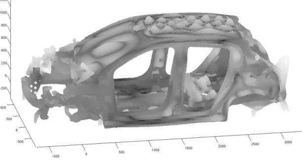
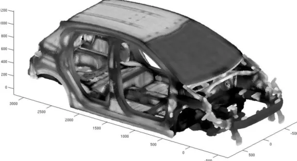
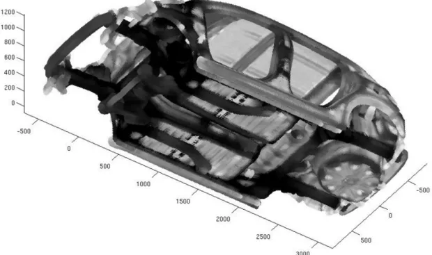
1.2 Position of the research 7 interface. Finally, Craig and Bampton [70] adapted the Hurty method. Improve-ments have been proposed with many variants [71, 72, 73, 74, 75], in particular for complex dynamical systems with many appendages considered as substructures (such as a disk with blades) Benfield and Hruda [76]. Another type of methods has been introduced in order to use the structural modes with free geometrical interface for two coupled substructures instead of the structural modes with fixed geometrical interface (elastic modes) as used in the Craig and Bampton method and as proposed by MacNeal [77] and Rubin [78]. The Lagrange multipliers have also been used to write the coupling on the geometrical interface [79, 80, 81, 82]. The substructuring techniques would require to discard the component modes associated with flexible sub-parts, hence removing their associated local displace-ments. Unfortunately, for the complex structures considered, there is no clear separation between the skeleton and the substructures for which the displace-ments would be local. For instance, with fixed thickness, the curvatures of a shell can lead to stiffened zones with respect to the rigidity of the flat zones. Con-sequently, in addition to the various embedded equipments within the structure, the complex geometry of the structure is responsible for the fact that there can be no separation of the several structural levels, but rather a continuous series of structural levels. In such conditions, the notion of local displacement is relative. Figures 1.6 and 1.7 show two complementary points of view of a car body

struc-Figure 1.6: Computational model of a car body structure, in which the gray intensity is related to the level of rigidity (the darker is the stiffer).

ture, in which it can be seen that a stiff skeleton emerges among several structural levels. In addition, there are numerous flexible parts spread over the whole struc-ture (not only well identified components such as the roof or the floor panels, but also erratically distributed flexible parts, see for instance the parts located at the front of the car). It allows for illustrating the fact that no clear boundary can be defined between the structural scales.

Figure 1.7: Computational model of a car body structure, in which the gray intensity is related to the level of rigidity (the darker is the stiffer).

It should be noted that, in contrast to the usual long-wavelength global displace-ments of the LF band, the local displacedisplace-ments associated with the structural sub-levels, which can then also appear in the LF band, are characterized by short wavelengths, similarly to HF displacements. As a result, for the complex struc-tures considered, there is an overlap of the three vibration regimes, LF, MF, and HF.

Concerning the taking into account of uncertainties in the computational model, the probabilistic framework is well adapted to construct the stochastic models, for the stochastic solvers, and for solving the associated statistical inverse problems for the identification of the stochastic models, for the finite dimension and for the infinite dimension. Hereinafter, we present a brief background that is limited to

1.2 Position of the research 9 the probabilistic framework for uncertainty quantification. As a function of the sources of uncertainties in the computational model (model-parameter uncertain-ties and model uncertainuncertain-ties induced by modeling errors) and of the variabiliuncertain-ties in the real dynamical system, several probabilistic approaches can be used. (i) Output-predictive error method. Several methods are currently available for analyzing model uncertainties. The most popular one is the standard output-predictive error method introduced in [83]. This method has a major drawback because it does not enable the ROM to learn from data.

(ii) Parametric probabilistic methods for model-parameter uncertainties. An alter-native family of methods for analyzing model uncertainties is the family of para-metric probabilistic methods for the uncertainty quantification. This approach is relatively well developed for model-parameter uncertainties, at least for a reason-ably small number of parameters. It consists in constructing prior and posterior stochastic models of uncertain model parameters pertaining, for example, to ge-ometry, boundary conditions, material properties, etc [84, 85, 86, 87, 88, 89, 90, 91, 92, 93, 94, 95, 96]. This approach was shown to be computationally efficient for both the computational model and its associated ROM (for example, see [97, 98]), and for large-scale statistical inverse problems [99, 100, 101, 102, 103, 104]. How-ever, it does not take into account neither the model uncertainties induced by modeling errors introduced during the construction of the computational model, nor those due to model reduction.

(iii) Nonparametric probabilistic approach for modeling uncertainties. For model-ing uncertainties due to more general modelmodel-ing errors, a nonparametric prob-abilistic approach was introduced in [105], in the context of linear structural dynamics. The methodology is in two steps. For the first one, a linear ROM of dimension n is constructed by using the linear computational model with m degrees of freedom (DOFs) and a ROB of dimension n. For the second step, a linear stochastic ROM is constructed by substituting the deterministic matri-ces underlying the linear ROM with random matrimatri-ces for which the probability distributions are constructed using the Maximum Entropy (MaxEnt) principle [106, 107]. The construction of the linear stochastic ROM is carried out under the constraints generated from the available information such as some algebraic properties (positiveness, integrability of the inverse, etc.) and some statistical information (for example, the equality between mean and nominal values). This nonparametric probabilistic approach has been extended for different ensembles of random matrices and for linear boundary value problems [108, 109]. It was also experimentally validated and applied for linear problems in composites [110], vis-coelasticity [111], dynamic substructuring [112, 113, 114], vibroacoustics [44, 43], robust design and optimization [115], etc. More recently, the nonparametric ap-proach has been extended to take into account some nonlinear geometrical effects

in structural analysis [116, 117], but it does not hold for arbitrary nonlinear sys-tems, while the work recently published [118] allows for taking into account any nonlinearity in a ROM.

In addition, the real systems exhibit variabilities: for a given design of a structure, the associated manufactured objects exhibit variations, which result in dispersed FRFs. It can be explained by the manufacturing process and by the small dif-ferences in the design configurations. It should be noted that, in general, the variability of the real system increases with the frequency. Figure 1.8 presents a set of 20 trajectories obtained measuring, under the same conditions, the FRF (modulus in log scale of the acceleration at a given location) of 20 nominally iden-tical automobiles. One can see that the dispersion increases with the frequency.

200 400 600 800 1000 1200 1400 −80 −70 −60 −50 −40 −30 −20 −10 Frequency (Hz) Acceleration (dB,m/s 2 )

Figure 1.8: Experimental measurements of 20 FRFs on a broad frequency band performed on PSA cars of the same type [119].

1.3

Objectives of the research

As previously explained, for the complex structures considered, numerous local elastic modes are intertwined with the usual global elastic modes. The resulting high modal density and overlap of the LF, MF, and HF vibration regimes (pres-ence of small-wavelength HF-type displacements with the usual large-wavelength global displacements of the LF band) induces two major difficulties, pertaining to uncertainty quantification and to computational efficiency.

1.4 Strategy of the research 11 The objective of this thesis is thus double. First, to provide a multilevel stochastic ROM that is able to take into account the heterogeneous variability introduced by the overlap of the three vibration regimes. Second, to provide a predictive ROM whose dimension is decreased with respect to the classical ROM constructed by using the modal analysis method. Both these objectives are to be fulfilled by means of efficient methods that are non-intrusive with respect to commercial soft-ware.

1.4

Strategy of the research

Recently, a new methodology [120] has been proposed for constructing a stochas-tic ROM devoted to dynamical structures having numerous local elasstochas-tic modes in the low-frequency range. The stochastic ROM is obtained by implementing the nonparametric probabilistic approach of uncertainties within a novel ROM whose ROB is constituted of two families: one of global displacements and an-other of local displacements. These families are obtained through the introduc-tion, for the kinetic energy, of a projection operator associated with a subspace of piecewise constant functions. The spatial dimension of the subdomains, in which the projected displacements are constant, and which constitute a parti-tion of the domain of the structure, allows for controlling the filtering between the global displacements and the local displacements. These subdomains can be seen as macro-elements, within which, using such an approximation, no local displacement is permitted. It should be noted that the generation of a domain partition for which the generated subdomains have a similar size (that we call uniform domain partition), necessary for obtaining a spatially uniform filtering

criterion, is not trivial for complex geometries. Based on the Fast Marching

Method [121, 122], a general method has been developed in order to perform the uniform domain partition for a complex finite element mesh, and then imple-mented for the case of automobile structures [45, 46]. Published papers related to the methodology are given in [120, 45, 46, 123, 124]. Related to a part of these papers, a former PhD thesis [125] was defended in 2012. In the present thesis (see [126, 127, 128, 129, 130, 131, 132]), the filtering methodology is generalized through the introduction of a computational framework for the use of any arbitrary approximation subspace for the kinetic energy, in place of the piecewise constant approximation. In particular, polynomial shape functions (with support the whole domain of the structure) are used for constructing a global-displacements ROM for an automobile. This generalization allows for carrying out an efficient con-vergence of the global-displacements ROM with respect to the so-defined filtering

(in contrast, constructing several uniform domain partitions of different charac-teristic sizes can be, in practice, very time-consuming). In addition, a multilevel ROM is introduced, whose ROB is constituted of several families of displacements, which correspond to the several structural levels of the complex structure. More precisely, a multilevel ROM whose ROB is constituted of three families, namely the LF-, MF-, and HF-type displacements (successively, using several filterings), is presented. The multilevel ROM allows for implementing a probabilistic model of uncertainties that is adapted to each vibration regime. This way, the amount of statistical fluctuations for the LF-, MF-, and HF-type displacements can be controlled using the multilevel stochastic ROM that is obtained.

An alternative construction of a multilevel stochastic ROM has been proposed in [129], but for which the implementation by using the non-intrusive algorithm proposed in this thesis would not be possible.

It should be noted that multilevel substructuring techniques can be found in the literature [133, 134, 135], but for which the purpose is to accelerate the solution of large-scale generalized eigenvalue problems.

1.5

Manuscript layout

The thesis is organized as follows. In Chapter 2, the reference computational model is introduced, followed by the classical construction of the ROM that is performed by using modal analysis, on which the classical stochastic ROM is then implemented by using the nonparametric probabilistic approach of uncertainties. In Chapter 3, the methodology devoted to the filtering of the global and of the local displacements is presented, which is then used in Chapter 4 for defining the multilevel ROM. In this chapter, the numerical procedure is also detailed and the construction of the multilevel stochastic ROM is given. Finally, in Chapter 5, the proposed methodology is applied to an automobile, for which the multilevel stochastic ROM is identified by using experimental measurements, and for which its results are compared to those of the classical stochastic ROM.

Chapter 2

Classical reduced-order model

In this chapter, in addition to the reference computational model, we present the very well known modal analysis method as well as the construction of the asso-ciated stochastic ROM that is obtained by using the nonparametric probabilistic approach of uncertainties [105]. This way, basic notions that will be reused later are introduced. In addition, the multilevel stochastic ROM proposed in this work will be compared to latter classical stochastic ROM.

2.1

Reference computational model

The vibration analysis is performed over a broad frequency band – denoted as B – by using the finite element method. Let m denote the dimension (number of DOFs) of the finite element model. For all angular frequency ω belonging to

B = [ωmin, ωmax], the m-dimensional complex vector U(ω) of displacements is the

solution of the matrix equation,

( −ω2_{[M] + iω[D] + [K] ) U(ω) = F(ω) ,} (2.1)

in which F(ω) is the m-dimensional complex vector of the external forces and where, assuming the structure is fixed on a part of its boundary, [M], [D], and [K] are the positive-definite symmetric (m × m) real mass, damping, and stiffness matrices.

In practice, dimension m of the reference (or high-fidelity) computational model can be very high (millions of DOFs). Nevertheless, matrices [M], [D], and [K] are sparse. However, Eq. (2.1) has to be solved for the frequency sampling and possibly, for several external loadings. In addition, whole this computation must

be done several times for implementing the Monte-Carlo method for uncertainty quantification and also, for instance, in the context of a robust design, for which a sampling of the design parameters has to be considered. In this context and for complex structures, the introduction of ROMs is necessary for making such computation tractable. In this thesis, we consider ROMs that are defined upon their projection basis (that is to say their ROB), and which consist in using this projection basis in order to project the equations associated with the reference computational model. The ROB has to be constructed so that the associated vector subspace consists of a good representation of the solution of the dynamical problem. The steps for constructing the ROM are often referred to as the offline stage, and the stage during which the ROM is used for performing the actual simulation (including design optimization, stochastic analysis, etc.) is referred to as the online stage. It should be noted that, in this context, the reduction of the computational effort devoted to the offline stage is not of the greatest concern. Instead, the reduction of the computational effort devoted to the online stage, made possible through the use of a small-dimension ROM, is of great interest for handling large-scale simulations (independently of the computational effort required for the construction of the ROM). In next Section 2.2, the classical ROM, for which the ROB is constituted of the first elastic modes, is presented. For complex structures exhibiting numerous local elastic modes as soon the LF band, the solution of the generalized eigenvalue problem associated with the conservative linear dynamical system, for which the eigenvectors are the elastic modes, can involve a great computational effort (corresponding to the offline stage), due to the high modal density resulting from the presence of the local elastic modes. It should be noted that this increased computational effort for the offline stage is negligible compared to the increased computational effort induced by the use of a high-dimension ROM for the online stage (high dimension due to the presence of numerous local elastic modes in the ROB). In Chapter 3, a methodology for the construction of a small-dimension ROM is presented, based on the use of a ROB that is constituted of global displacements.

2.2

Classical nominal reduced-order model

For all α = 1, . . . , m the elastic modes ϕα with associated eigenvalues λα are the

solutions of the generalized eigenvalue problem,

2.3 Classical stochastic reduced-order model 15

The first n eigenvalues verify 0 < λ1 ≤ λ2 ≤ . . . ≤ λn < +∞ and the

normaliza-tion that is chosen for the eigenvectors is such that

[Φ]T_{[M][Φ] = [I}n] , (2.3)

in which [Φ] = [ϕ1. . . ϕn], and where [In] is the identity matrix of dimension

n. Such a normalization with unit generalized mass is always adopted in this document, in which several generalized eigenvalue problems are introduced. In practice, only the first n elastic modes with n  m (associated with the lowest

eigenvalues or lowest eigenfrequencies fα =

√

λα/2π in Hz) are calculated. The

(m × n) real matrix [Φ] is the ROB of the classical nominal reduced-order model (C-NROM). The vector subspace spanned by the ROB of the C-NROM is denoted

by Sc. Using the C-NROM, displacements U(ω) belong to Sc and we have

U(ω) ' [Φ]q(ω) =

n

X

α=1

qα(ω) ϕα, (2.4)

where the n-dimensional complex vector of generalized coordinates q(ω) = (q1(ω)

. . . qn(ω)) is the solution of the reduced-matrix equation,

( −ω2[M] + iω[D] + [K] ) q(ω) = f(ω) , (2.5)

in which f(ω) = [Φ]T_{F(ω), [D] = [Φ]}T_{[D][Φ] is, in general, a full matrix, and where}

diagonal matrices [K] and [M] are such that

[K] = [Φ]T_{[K][Φ] = [Λ] ,} [M] = [Φ]T_{[M][Φ] = [I}n] , (2.6)

in which [Λ] is the matrix of the first n eigenvalues.

2.3

Classical stochastic reduced-order model

The classical stochastic reduced-order model (C-SROM) is constructed by us-ing the nonparametric probabilistic approach of uncertainties [105] within the C-NROM. In this nonparametric approach, each nominal reduced matrix of di-mension n, say [A] (= [M], [D], or [K]), is replaced by a random matrix, [A] (= [M], [D], or [K]), whose probability distribution has been constructed by using the maximum entropy principle [106, 107] under the following constraints:

• Matrix [A] is with values in the set of all the positive-definite symmetric (n × n) real matrices.

chosen as the nominal matrix.

• E{||[A]−1||2_F} < +∞ , with ||.||F the Frobenius norm, for insuring the

exis-tence of a second-order solution of the stochastic ROM. The construction of random matrix [A] is given by

[A] = [LA]T[Gn(δA)][LA] , (2.7)

where, using the Cholesky factorization [A] = [LA]T[LA] with upper-triangular

[LA], the random matrix [Gn(δA)] , whose construction is given in [105], is

positive-definite almost surely, with mean value [In], and is parameterized by a dispersion

parameter δA that is defined by

δ_A2 = 1

nE{||[Gn(δA)] − [In]||

2

F} . (2.8)

Hyperparameter δA of random matrix [Gn(δA)] has to verify 0 < δ < δmax, with

δmax given by

δmax =

r n + 1

n + 5. (2.9)

The construction of [Gn(δA)] proceeds from the application of the maximum

en-tropy principle under the following constraints:

• Matrix [Gn(δA)] is with values in the set of all the positive-definite

symmet-ric (n × n) real matsymmet-rices.

• E{[Gn(δA)]} = [In] .

• E{||[Gn(δA)]

−1

||2_F} < +∞ .

We now give the results for the random generation of matrix [Gn(δA)]. It can be

written as [Gn(δA)] = [LG(δA)]T [LG(δA)] , in which the (n × n) upper-triangular

random matrix [LG(δA)] is defined through its components as:

for i < j [LG(δA)]_ij = δA(n + 1) −1/2 Uij, (2.10) for i = j [LG(δA)]_ij = δA(n + 1)−1/2 p 2Vi, (2.11)

in which the random variables {Uij}ij are independent copies of a standard Normal

random variable and where the random variables {Vi}i are independent and are

2.3 Classical stochastic reduced-order model 17

1 + δ2

A(1 − i)) depending on i and with rate parameter β = 1. The expression for

the gamma distribution fG is the following,

fG(x; α, β) =

βα_xα−1_e−xβ

Γ(α) , (2.12)

in which gamma function Γ(α) is given by

Γ(α) =

Z +∞

0

tα−1e−tdt . (2.13)

Using the Monte-Carlo simulation method [136], the C-SROM allows for comput-ing the random displacements U(ω) associated with U(ω),

U(ω) = [Φ]Q(ω), (2.14)

in which the random complex vector Q(ω) of the generalized coordinates is ob-tained by solving the random matrix-equation,

( −ω2[M] + iω[D] + [K] ) Q(ω) = f(ω) . (2.15)

The Monte-Carlo simulation method consists in performing the calculation sev-eral times using realizations of the random variables involved in the probabilistic model. In Eq. (2.15), it allows for propagating uncertainties from the system ma-trices [M], [D], [K] to the output FRFs U(ω).

The classical ROM presented in this Section 2 is built upon the use of the elastic modes that are present in frequency band of analysis B (or a little further). In this manner, the size of the model is reduced while preserving its accuracy for this band. For the complex structures under consideration, numerous local dis-placements are intertwined with the global disdis-placements. As a result, among the elastic modes present in B, many have little contribution to the robust dynamical response of the stiff skeleton of the structure that is provided by the C-SROM. Consequently, we present the construction of an adapted ROM that is based on a ROB from which some local displacements have been filtered.

Chapter 3

Global-displacements

reduced-order model

In this chapter, we present the construction of a new ROM that is based on the use of a global-displacements ROB, instead of the classical ROB of elastic modes, susceptible to include numerous local displacements. In Section 3.1, we present the construction of an unusual mass matrix that is associated with a reduced kinematics for the kinetic energy. In Section 3.2, we use this mass matrix for obtaining unusual eigenvectors that constitute the global-displacements ROB (this unusual mass matrix is not used as the mass matrix for computing the response of the dynamical system). In section 3.3, an efficient and nonintrusive algorithm is proposed for implementing the ROB. Finally, in Section 3.4, we give the construction of a ROB that is constituted of the complementary local displacements that are neglected in the global-displacements ROM.

3.1

Reduced kinematics for the kinetic energy

In order to filter local displacements, a reduced kinematics is introduced for the mass matrix. This reduced kinematics is intended to be such that the local dis-placements cannot be represented. Instead of using local shape functions within the usual finite elements, we propose the use of r global shape functions, which

span a vector subspace, SR, and which constitute the columns of a (m × r) real

matrix, [B]. It should be noted that the support of these shape functions is the whole domain of the structure and that they are approximated within the finite element basis. In this work, the reduced kinematics used consists of polynomial shape functions.

3.1.1

Construction of the polynomial basis

The objective of this section is the construction of basis matrix [B] of subspace

SR. For all m-dimensional vector v belonging to SR, there exists a r-dimensional

real vector, c , such that

v = [B] c . (3.1)

In the work initialized in [120], the construction of the reduced kinematics is based

on a uniform domain partition of the struture, Ω, into Nssubdomains Ω1, . . . , ΩNs.

For complex finite element models, such domain partitioning is not a straightfor-ward task. In [45, 46], uniform domain partitions of the finite element mesh of automobiles were performed using an algorithm [45] based on the Fast Marching Method [121, 122]. In this thesis, the use, for the kinematics reduction, of more accurate approximations (compared to the piecewise constant approximation), allows for avoiding such a domain partitioning.

3.1.1.1 Polynomial reduced kinematics

In this work, we propose a polynomial approximation of maximum degree d over

the entire domain Ω of the structure. To do so, Nµ multivariate orthogonal

poly-nomials p_α(µ) are used, where for µ = 1, . . . , N_µ multi-index α(µ) belongs to some

set Kd that is defined as follows. Let Kd be the set of vectors α = (α1, α2, α3) for

which integers α1, α2, and α3 verify

α3 ≤ α2 ≤ α1 ≤ d . (3.2)

It can be deduced (number of possible combinations) that,

Nµ= (d + 1)(d + 2)(d + 3)/6 . (3.3)

The orthogonality for the polynomials is defined with respect to mass matrix

[M] . Denoting as Nf the number of free nodes of the finite element model, the

approximate displacement v_γj of node γ ∈ {1, . . . , Nf} following direction j is

written as v_γj = Nµ X µ=1 p_α(µ)(x_γ) cj_µ, (3.4) in which cj

µ are the polynomials coefficients and where xγ = (xγ, yγ, zγ) is the

3.1 Reduced kinematics for the kinetic energy 21

the Nf equations associated with Eq. (3.4) can be rewritten as

vj = [ p ] cj, (3.5)

in which vj _{is the sub-vector of v constituted of the N}

f displacements vγj, cj is

the sub-vector of c constituted of the Nµcoefficients cjµ, and where the (Nf× Nµ)

real matrix [ p ] is constituted of the values, at each of the Nf mesh nodes, of each

of the Nµ polynomials pα(µ). It should be noted that the same N_µ polynomials

are used for every direction j. Basis matrix [B] of subspace SR, which is such

that v = [B] c, is then assembled using [ p ]. This assembly is such that only the 3 translational directions are considered for constructing the reduced kinematics. In order to make explicit the assembly, we give an example. Considering a given node γ of the finite element mesh for which we suppose there are 6 DOFs, namely the 3 translations and the 3 rotations, and for which the numerotation in the finite element model is such that the 3 rotations come after the 3 translations, the intersection, with the 3 columns associated with the number-µ polynomial

p_α(µ), of the 6 rows in matrix [B] that are associated with node γ , is the following

sub-matrix, [ T_γµ] =          p_α(µ)(x_γ) 0 0 0 p_α(µ)(x_γ) 0 0 0 p_α(µ)(x_γ) 0 0 0 0 0 0 0 0 0          . (3.6)

As a consequence, for a three-dimensional dynamical system, the column

dimen-sion of matrix [B] is r = 3Nµ (which is the dimension of subspace SR, associated

with the reduced kinematics).

The definition for the multivariate orthogonal polynomials p_α(µ) is now given. For

this, using the same notation as for p_α(µ), the values, at the mesh nodes, of each

of the associated multivariate monomials, m_α(µ), can be written as

m_α(µ)(x_γ) = xα_γ1−α2yα_γ2−α3zα_γ3. (3.7)

Similarly to the definition of matrix [ p ], let [ m ] be the (Nf × Nµ) real matrix

that is constituted of the Nf values, at the mesh nodes, of each of the Nµ

mono-mials m_α(µ). Matrix [ m ] of the discrete monomials being introduced, the explicit

construction for [ p ] is the following. Matrix [ p ] is constructed as an orthonormal-ization of [ m ], with respect to mass matrix [M]. To do so, a QR decomposition

is performed.

Remark 1 For the case of the use of a diagonally-lumped approximation for

mass matrix [M] (approximation for which we suppose the nodal mass is inde-pendent of the translational direction), the computation of matrix [ p ] is

car-ried out by performing the thin QR decomposition of the (Nf × Nµ) real matrix

[ a ] = [m`<sub>]</sub>1/2<sub>[ m ], in which [m</sub>`_{] is the diagonal matrix constituted of the N}

f nodal

masses. The QR decomposition is written as

[ a ] = [ q ][ r ] , (3.8)

in which [ r ] is a (Nµ× Nµ) real matrix and where [ q ] is a (Nf× Nµ) real matrix,

which verifies

[ q ]T[ q ] = [INµ] . (3.9)

Matrix [ p ] can then be obtained by using [ p ] = [m`_]−1/2_{[ q ]. Pre-multiplying}

latter equation by [m`_]1/2 _{and using Eq. (3.9) yields the orthogonality property}

for the multivariate polynomials,

[ p ]T[m`][ p ] = [INµ] . (3.10)

It should be noted that, in practice, the computation of [ p ] is not necessary (which

allows the inversion of diagonal matrix [m`] to be circumvented, useful if some

diagonal terms in [m`] were to be zero). Instead, in order to construct the mass

matrix corresponding to the polynomial approximation, which will be defined in

next Section 3.1.2, only the product [m`_]1/2_{[ q ] is required.}

Remark 2 The use of orthogonal polynomials allows for obtaining an

orthonor-malized basis matrix [B], which verifies

[B]T_{[M][B] = [I}r] . (3.11)

It should be noted that this step (the orthogonalization) is important with

re-spect to the effectiveness of the method. In Section 3.1.2.1, the inversion of

the reduced matrix in Eq. (3.11) is involved in the construction of a projector (orthogonal-projection matrix) that is used for the kinematics reduction of the mass matrix. Without the orthogonalization step, round-off errors would lead to an ill-conditioned reduced matrix (or even a rank-deficient one) and/or to large errors.

3.1 Reduced kinematics for the kinetic energy 23 Deformation shapes via orthogonal projections onto polynomial bases In order to illustrate the effect of using such a polynomial approximation, which we recall to be devoted to the filtering of local displacements, we consider the orthogonal projection, onto the polynomial basis (represented by matrix [B]), of a regular low-frequency elastic mode of a car body structure. This elastic mode, depicted in Fig. 3.1, includes displacements of several structural scales, including (i) a global deformation of the body structure, (ii) a local deformation of the roof, and (iii) a highly local deformation of a flexible part that is located at the left back. The polynomial approximation is parameterized by the maximum degree d used for the polynomials. The filtering is thus controlled by the value of d. For different values of d, namely d = 5, d = 10, d = 15, and d = 20, the orthogonal projection of the low-frequency elastic mode is performed. The results are plotted in Figs. 3.2 to 3.5. It can be seen that, for the orthogonal projection given by d = 5, both scales of local displacements have been filtered. For the orthogonal projection given by d = 15, the first scale of local displacements, associated with the roof, is recovered. Finally, for the orthogonal projection given by d = 20, the original mode shape is recovered (including all the scales of displacements).

Figure 3.1: Mode shape of a regular low-frequency elastic mode of a car body structure (eigenfrequency 72 Hz).

Figure 3.2: Deformation shape of the orthogonal projection, onto the polynomial basis of maximum degree d = 5, of the elastic mode shown in Fig. (3.1).

Figure 3.3: Deformation shape of the orthogonal projection, onto the polynomial basis of maximum degree d = 10, of the elastic mode shown in Fig. (3.1).

3.1 Reduced kinematics for the kinetic energy 25

Figure 3.4: Deformation shape of the orthogonal projection, onto the polynomial basis of maximum degree d = 15, of the elastic mode shown in Fig. (3.1).

Figure 3.5: Deformation shape of the orthogonal projection, onto the polynomial basis of maximum degree d = 20, of the elastic mode shown in Fig. (3.1).

3.1.1.2 Alternative reduced kinematics

The proposed reduced kinematics, which is presently applied to whole domain

Ω, can also be applied for each subdomain Ω1, . . . , ΩNs of a partition of Ω. If

such a partition is introduced, and if the maximum degree d of the polynomial approximation is chosen, for each subdomain, as d = 0 (which corresponds to a constant displacement field by subdomain), we then obtain the formulation introduced in [120]. In such a case, for the continuous formulation, a projection

operator hr _{of the displacement field u onto the subspace of constant functions}

by subdomain is, for all x in Ω , written as

{hr_{(u)} (x) =} Ns X j=1 1Ωj(x) 1 mj Z Ωj ρ(x0)u(x0)dx0, (3.12)

in which 1Ωj(x) = 1 if x ∈ Ωj and is zero otherwise, where mj =

R

Ωjρ(x)dx is

the mass of subdomain Ωj, and where ρ is the mass density. In [120], the finite

element discretization [Hr_{] of h}r _{is used for obtaining the mass matrix associated}

with the reduced kinematics, [Mr_{] = [H}r_]T

[M] [Hr_].

On the other hand, if the maximum degree d of the polynomial approximation is chosen, for each subdomain, as d = 1, then the reduced kinematics is very close to a rigid-body displacements field by subdomain as proposed in [128].

Figure 3.6 presents the case of a heterogeneous plate for which two distinct struc-tural levels can be defined: the first one consists of a stiff skeleton and the second one of 12 flexible panels that are attached to the stiff skeleton. For this struc-ture, numerous local displacements (associated with isolated vibrations of the flexible panels) are intertwined with the global displacements (associated with long-wavelength vibrations of the stiff skeleton). In order to filter the local dis-placements, a uniform domain partition of the structure is introduced. Two differ-ent approximations are used: a piecewise constant approximation and a piecewise linear approximation. For an elastic mode including both global and local dis-placements, both of these reduced kinematics allow the associated orthogonal projections to get rid of the local displacements of the flexible panels. In addi-tion, for this case, it can be seen that, in comparison to the piecewise constant approximation, the piecewise linear approximation allows for obtaining a better approximation of the original deformation shape of the stiff skeleton, while the local displacements of the flexible panels remain filtered.

3.1 Reduced kinematics for the kinetic energy 27

Figure 3.6: Case of a heterogeneous plate including two structural scales (with a stiff main frame supporting 12 flexible panels): undeformed configuration (top-left), an elastic mode exhibiting both global and local displacements (top-right), its orthogonal projection onto a subspace of piecewise constant functions (bottom-left), and its orthogonal projection onto a subspace of piecewise linear functions (bottom-right).

3.1.2

Reduced-kinematics mass matrix

It should be noted that in the case where both the kinetic and elastic energies were to be calculated using this polynomial approximation, the associated mass and

stiffness matrices would be of reduced dimension (r × r) and given by [B]T_[M][B]

and by [B]T_{[K][B], respectively (which corresponds to a Galerkin projection, as}

used throughout all the document). In the present work, the strategy employed consists in approximating the kinetic energy while keeping the elastic energy ex-act. The construction of an unusual mass matrix, corresponding to the reduced kinematics, and which is compatible with keeping [K] as the stiffness matrix, is given. In the following, such an unusual mass matrix will be referenced as the reduced-kinematics mass matrix.

3.1.2.1 Definition

First, the kinetic energy Ek(V(t)) associated with any time-dependent real velocity

vector V(t) of dimension m is given by

Ek(V(t)) =

1

2V(t)

T

[M]V(t) . (3.13)

Let then Vr(t) be the orthogonal projection of V(t) onto subspace SR, with respect

to the inner-product defined by matrix [M]. It can be written as

Vr(t) = [B] copt(V(t)) , (3.14)

in which copt

(V(t)) is the unique solution of the optimization problem,

copt

(V(t)) = arg min

c ∈ Rr(V(t) − [B] c)

T

[M] (V(t) − [B] c) , (3.15)

and which can be shown to be given by

copt

(V(t)) = ( [B]T [M] [B] )−1[B]T_{[M] V(t) .} (3.16)

Assuming the columns of [B] to be orthonormalized with respect to [M] (see

Eq. (3.11)), the projector [P] that is such that Vr(t) = [P]V(t) is therefore written

as

3.1 Reduced kinematics for the kinetic energy 29 the latter being a (m × m) real matrix of rank r ≤ m . As a result, the reduced

kinetic energy, defined as Er

k(V(t)) = Ek(Vr(t)), can be written as

E_kr_{(V(t)) =} 1

2V(t)

T

[Mr]V(t) , (3.18)

in which the m-dimensional reduced-kinematics mass matrix,

[Mr] = [P]T[M][P] , (3.19)

is of rank r ≤ m , and can be written, using Eqs. (3.11), (3.17), and (3.19), as

[Mr] = [M][B][B]T[M] . (3.20)

3.1.2.2 Positiveness and null space

Since matrix [M] is positive definite, from Eq. (3.19) it can be deduced that the

null space of [Mr_{] is equal to the null space of [P] . The null space of [P] , which we}

denote as S_R⊥, is the orthogonal complement of subspace SR of Rm, with respect

to the inner-product given by matrix [M]. In other words, for all m-dimensional real vector x , we have

x = xr+ xc, (3.21)

in which vectors xr _{= [P] x ∈ S}

R and xc= ([Im] − [P]) x ∈ SR⊥ verify

xc T_{[M] x}r= 0 . (3.22)

The notion of orthogonal complement will be involved again later. Since dimension

r of SR is such that r ≤ m, matrix [Mr] is positive semidefinite.

3.1.2.3 Residual kinetic energy minimization

From Eqs. (3.13), (3.14), (3.15) and (3.22), it can be deduced that the construction

proposed is such that the residual kinetic energy, Ek(V) − Ek(Vr), verifying

Ek(V) − Ek(Vr) = Ek(V − Vr) , (3.23)

is minimum.

3.1.2.4 Mass conservation

Let mtot _{be the positive number such that m}tot ₌ 1

31

T _{[M] 1, in which the}

for the rotation DOFs (if there exist in the computational model). Quantity mtot

represents approximately the mass of the structure (the mass located on the fixed

boundary conditions is not taken into account). If 1 belongs to SR (in which case

[P] 1 = 1), then the mass mtot,r ₌ 1

31 T

[Mr] 1 is such that mtot,r _{= m}tot_{. Since}

vector 1 is spanned by the 3 columns of matrix [B] corresponding to polynomial

p_α(1) (order-0 polynomial with multi-index α(1) = (0, 0, 0)), it can be deduced

that for any maximum degree d of the polynomial approximation, the mass is conserved within the kinematics reduction.

3.2

Global-displacements reduced-order basis

In order to span the global-displacements space, denoted by Sg (and which is a

subspace of Rm), mass matrix [M] is replaced by [Mr] for obtaining the generalized

eigenvalue problem (that differs from the one used for computing the elastic modes and that cannot be used for computing them),

[K]ψαg = σαg[Mr]ψαg, (3.24)

in which the eigenvectors ψg

α consist of global displacements and where σgα are

the associated eigenvalues. The first r eigenvalues are such that 0 < σg₁ ≤ σg₂ ≤

. . . ≤ σg

r < +∞ and the eigenvalues of rank greater than r are all infinite, their

associated eigenvectors being orthogonal to vector subspace SR.

It should be noted that (i) the r eigenvectors ψg

αare not orthogonal with respect to

mass matrix [M] and (ii) they will be used for the projection of the computational

model defined by Eq.(2.1), which involves mass matrix [M] and not [Mr]. Let

us introduce the (m × ν) real matrix, [Ψg] = [ψg₁. . . ψg_ν], in which ν is a given

truncation order such that

ν ≤ r . (3.25)

The global-displacements ROB is then defined by the first eigenvectors of the dynamical system, which are constrained to belong to the vector space spanned

by the ν columns of the (m × ν) real matrix [Ψg_{]. The global-displacements ROB}

is denoted by [Φg_{] whose columns ϕ}g

α are thus written as

ϕg_α = [Ψg]rα, (3.26)

3.2 Global-displacements reduced-order basis 31 problem,

([Ψg]T_[K][Ψg]) rα = λgα([Ψ

g

]T_[M][Ψg]) rα. (3.27)

The eigenvalues verify 0 < λg₁ ≤ λg₂ ≤ . . . ≤ λg

ν < +∞ . Introducing the matrix

[R] such that [R] = [r1. . . rng], in which ng is a given truncation order that will

be defined hereinafter, matrix [Φg_{] can be rewritten as}

[Φg] = [Ψg][R] , (3.28)

which, using Eq. (3.27) and recalling our choice of a unit generalized mass nor-malization, yields

[Φg]T_[K][Φg] = [Λg] , [Φg]T_[M][Φg] = [Ing] , (3.29)

with [Λg_{] the diagonal matrix of the first n}

g eigenvalues λgα. Only the first ng

eigenvectors (associated with the lowest frequencies f_αg = √λgα/2π) are kept for

constituting [Φg] = [ϕg₁. . . ϕg_ng]. Dimension ng of global-displacements subspace

Sg is deduced from a cutoff frequency, fc, for which ng verifies

f_ng_g ≤ fc_{. (3.30)}

In addition, ng satisfies the inequality,

ng ≤ ν . (3.31)

Cutoff frequency fc is a data that must be chosen greater or equal to the

up-per bound ωmax/2π of frequency band B and that must be adjusted through the

analysis of the FRFs. It should be noted that truncation order ν cannot directly

be deduced from the value √σgν/2π because the eigenvalues σ_αg are not the

eigen-frequencies of the dynamical system. For ν ≤ r, the following inequality can be shown,

λg_ν ≤ σg

ν, (3.32)

for which, in addition, the difference between λg

ν and σgν can be significant.

For brevity, no notation is introduced for the equations related to the global-displacements ROM, which would be similar to Eqs. (2.4) and (2.5) and which, anyway, would not be used.