HAL Id: tel-01966770
https://tel.archives-ouvertes.fr/tel-01966770
Submitted on 29 Dec 2018
HAL is a multi-disciplinary open access
archive for the deposit and dissemination of sci-entific research documents, whether they are pub-lished or not. The documents may come from teaching and research institutions in France or abroad, or from public or private research centers.
L’archive ouverte pluridisciplinaire HAL, est destinée au dépôt et à la diffusion de documents scientifiques de niveau recherche, publiés ou non, émanant des établissements d’enseignement et de recherche français ou étrangers, des laboratoires publics ou privés.
Micro-Data Reinforcement Learning for Adaptive
Robots
Konstantinos Chatzilygeroudis
To cite this version:
Konstantinos Chatzilygeroudis. Micro-Data Reinforcement Learning for Adaptive Robots. Robotics [cs.RO]. Universite de Lorraine, 2018. English. �NNT : 2018LORR0276�. �tel-01966770�
´
Ecole doctorale IAEM Lorraine
Micro-Data Reinforcement Learning
for Adaptive Robots
TH`
ESE
pr´esent´ee et soutenue publiquement le 14 December 2018 pour l’obtention du
Doctorat de l’Universit´
e de Lorraine
(mention informatique) par
Konstantinos Chatzilygeroudis
Composition du jury
Rapporteurs : Pierre-Yves OUDEYER Directeur de recherche
Inria Bordeaux Sud-Ouest, France Yiannis DEMIRIS Professor
Imperial College London, UK
Examinateurs : Aude BILLARD Professor
EPFL, Switzerland Alain DUTECH Charg´e de recherche
Inria, CNRS, Universit´e de Lorraine, France Verena V. HAFNER Professor
Humboldt-Universit¨at zu Berlin, Germany Directeur : Jean-Baptiste MOURET Directeur de recherche
Inria, CNRS, Universit´e de Lorraine, France
Laboratoire Lorrain de Recherche en Informatique et ses Applications — UMR 7503
bots
English Abstract
Robots have to face the real world, in which trying something might take seconds, hours, or even days. Unfortunately, the current state-of-the-art reinforcement learning algorithms (e.g., deep reinforcement learning) require big interaction times to find effective policies. In this thesis, we explored approaches that tackle the challenge of learning by trial-and-error in a few minutes on physical robots. We call this challenge “micro-data reinforcement learning”.
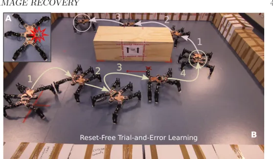
In our first contribution, we introduced a novel learning algorithm called “Reset-free Trial-and-Error” that allows complex robots to quickly recover from unknown circumstances (e.g., damages or different terrain) while completing their tasks and taking the environment into account; in particular, a physi-cal damaged hexapod robot recovered most of its locomotion abilities in an environment with obstacles, and without any human intervention.
In our second contribution, we introduced a novel model-based reinforce-ment learning algorithm, called Black-DROPS that: (1) does not impose any constraint on the reward function or the policy (they are treated as black-boxes), (2) is as data-efficient as the state-of-the-art algorithm for data-efficient RL in robotics, and (3) is as fast (or faster) than analytical approaches when several cores are available. We additionally proposed Multi-DEX, a model-based policy search approach, that takes inspiration from novelty-based ideas and effectively solved several sparse reward scenarios.
In our third contribution, we introduced a new model learning procedure in Black-DROPS (we call it GP-MI) that leverages parameterized black-box priors to scale up to high-dimensional systems; for instance, it found high-performing walking policies for a physical damaged hexapod robot (48D state and 18D action space) in less than 1 minute of interaction time.
Finally, in the last part of the thesis, we explored a few ideas on how to incorporate safety constraints, robustness and leverage multiple priors in Bayesian optimization in order to tackle the micro-data reinforcement learning challenge.
Throughout this thesis, our goal was to design algorithms that work on physical robots, and not only in simulation. Consequently, all the proposed approaches have been evaluated on at least one physical robot. Overall, this thesis aimed at providing methods and algorithms that will allow physical robots to be more autonomous and be able to learn in a handful of trials.
French Abstract
Les robots op`erent dans le monde r´eel, dans lequel essayer quelque chose prend des secondes, des heures ou mˆeme des jours. Malheureusement, les algo-rithmes d’apprentissage par renforcement actuels (par exemple, les algoalgo-rithmes de “deep reinforcement learning”) n´ecessitent de longues p´eriodes d’interaction pour trouver des politiques efficaces. Dans ce th`ese, nous avons explor´e des algorithms qui abordent le d´efi de l’apprentissage par essai et erreur en quelques minutes sur des robots physiques. Nous appelons ce d´efi “Apprentissage par renforcement micro-data”.
Dans notre premi`ere contribution, nous avons propos´e un nouvel algorithme d’apprentissage appel´e “Reset-free Trial-and-Error” qui permet aux robots complexes de s’adapter rapidement dans des circonstances inconnues (par exemple, des dommages ou un terrain diff´erent) tout en accomplissant leurs tˆaches et en prenant en compte l’environnement; en particulier, un robot hexapode endommag´e a retrouv´e la plupart de ses capacit´es de locomotion dans un environnement avec des obstacles, et sans aucune intervention humaine.
Dans notre deuxi`eme contribution, nous avons propos´e un nouvel algo-rithme de recherche de politique “bas´e mod`ele”, appel´e Black-DROPS, qui: (1) n’impose aucune contrainte ´a la fonction de r´ecompense ou ´a la politique, (2) est aussi efficace que les algorithmes de l’´etat de l’art, et (3) est aussi rapide (ou plus rapide) que les approches analytiques lorsque plusieurs processeurs sont disponibles. Nous avons aussi propos´e Multi-DEX, une extension qui s’inspire de l’algorithme “Novelty Search” et permet de r´esoudre plusieurs sc´enarios o`u les r´ecompenses sont rares.
Dans notre troisi`eme contribution, nous avons introduit une nouvelle proc´edure d’apprentissage du mod`ele dans Black-DROPS qui exploite un simula-teur param´etr´e pour permettre d’apprendre des politiques sur des syst`emes avec des espaces d’´etat de grande taille; par exemple, cet extension de Black-DROPS a trouv´e des politiques de marche performantes pour un robot hexapode (espace d’´etat 48D et d’action 18D) en moins d’une minute de temps d’interaction.
Enfin, dans la derni`ere partie de la th`ese, nous avons explor´e quelques id´ees comment int´egrer les contraintes de s´ecurit´e, am´eliorer la robustesse et tirer parti des multiple a priori en optimisation bay´esienne.
A travers l’ensemble de cette th`ese, notre objectif ´etait de concevoir des algorithmes qui fonctionnent sur des robots physiques, et pas seulement en simulation. Par cons´equent, tous les approches propos´ees ont ´et´e ´evalu´ees sur au moins un robot physique. Dans l’ensemble, cette th`ese propose des
3 m´ethodes et des algorithmes qui permettre aux robots physiques d’ˆetre plus autonomes et de pouvoir apprendre en poign´ee d’essais.
Acknowledgements
The last three years and this thesis would not have been the same without the help and support of many people that I would like to warmly thank with these few lines.
First of all, from the bottom of my heart, I would like to thank my dear wife Eleni, for all the moments we shared together through the ups and downs of this three-year adventure. She has been extremely patient during the long evenings, nights and, sometimes, weekends that I spent to finish a paper, a long robotic experiment or simply some code. She has been my highest support during all these 3 years and the manuscript that you are currently reading would not have been the same without her.
Of course, this thesis would not have been of the same quality without the help by my supervisor, Jean-Baptiste Mouret. His supervision was discreet and tight at the same time. He really believed in me and my abilities, and gave me enough freedom to explore my own ideas. At the same time, he always kept a watching eye to prevent me from choosing dangerous roads that could hinder my route. His expectations, patience and useful advices have deeply shaped my scientific researching abilities. He taught me almost everything I know in scientific research and I am really proud of being one of his PhD students.
Within the ResiBots team and the LARSEN lab in general, I had the chance to collaborate and discuss with several excellent researchers and people. The members of the team were always very responsive, caring, friendly and I really enjoyed conversing with them. All the people of the LARSEN lab embraced me and Eleni warmly, and we felt from the first moment as a part of a big caring family. We are deeply grateful to all of them. I would like to thank some people in particular that I had the luck to meet and spend some more time with them (excluding the members of the ResiBots team that have their own dedicated thanks): Serena Ivaldi, Francis Colas, Kazuya Otani, Valerio Modugno, Pauline Maurice, Oriane Dermy, Sebastian Marichal, Olivier Buffet, Adrien Malais´e, I˜naki Fern´andez P´erez, Adrian Bourgaud, and Luigi Penco.
I would also like to thank all the members of the “ResiBots” team. Several interns, post-docs and collaborators passed, and we always laughed, joked and made a lot of pranks. In particular, I would like to thank Vassilis Vassiliades
5 for the long, constructive discussions and for the fellow researcher and friend that he has been, and still is, to me. This thesis surely would not have been the same without him. Additionally, I was very lucky to collaborate, discuss and spend some time with the excellent young researcher and student R´emi Pautrat. I gained a lot from this collaboration. I would also like to thank Vaios Papaspyros, Rituraj Kaushik, Federico Allocati, Roberto Rama, Jonathan Spitz, Dorian Goepp, Lucien Renaud, Brice Clement, Vladislav Tempez, Debaleena Misra and Kapil Sawant for all the nice discussions (scientific and not) that we had over the time we spent together and for our excellent collaboration.
I also had the chance to collaborate with some excellent researchers and I am really grateful to Shimon Whiteson, Supratik Paul, Sylvain Calinon and Freek Stulp for the wonderful collaborations that we had.
I was very fortunate to meet a lot of wonderful people in Nancy and to make some lifelong friends. Many thanks go to the three couples that we spent numerous nights drinking, laughing, discussing, sharing personal experiences and eating: Lazaros Vozikis-Chrysa Papantoniou, Nikolas Chrysikos-Lydia Schneider, Alexandros Petrelis-Maria Stathopoulou1. I would also like to thank the president of the association “Maison FrancoHell´enique Lorraine”, Katerina Karagianni, her wonderful husband Thierry Ca¨el and their adorable daughters, Ioanna and Marina, for making us feel like home and always being there for us. I would also like to thank all the members of the board of the association, and in particular, Bernard and Orthodoxia Salomon for always being helpful and available. Finally, I would like to thank Dimitris Chatziathanasiou, Vi-talis Ntombrougidis, Vassilis Vassiliades and Marianna Gregoriou, Annabelle Chapron and Nicolas Vicaire, Marianthi Elmaloglou, Dimitris Meimaroglou and Maria Prokopidou (and their wonderful kids, Eleni and Ioannis), Antonis Keremloglou and Marina Kotsani (and their little baby Symeon) for all the nice times that we spent together.
I would also like to thank my whole family for their endless support, love and encouragement: my parents (Ioannis and Maria), my sisters (Marianna, Theodora, Evangelia, Georgia), my brother (Gerasimos), my parents-in-law (Dimitrios and Giannoula) my brothers-in-law (Vassilis, Nikos, Michalis), my sister-in-law (Ourania) and my adorable nephews and nieces (Dimitrios, Ioanna and Anastasia).
I would also like to thank the members of the jury of my PhD defense for accepting to be part of the jury. It is truly an honor to be reviewed by such experienced and respected researchers. Finally, I would like also to thank the European Research Council and the University of Lorraine, who gave me the opportunity to pursue this PhD thesis.
1The order was decided by a random number generator because I could not put them in order!
Contents
Contents 6 List of Figures 8 List of Tables 10 1 Introduction 11 2 Background 18 2.1 Introduction . . . 18 2.2 Problem formulation . . . 20 2.3 Value-function approaches . . . 22 2.4 Policy Search . . . 232.5 Using priors on the policy parameters or representation . . . 27
2.6 Learning models of the expected return . . . 31
2.7 Learning models of the dynamics . . . 37
2.8 Other approaches . . . 44
2.9 Conclusion . . . 45
3 Reset-free Trial and Error for Robot Damage Recovery 47 3.1 Introduction . . . 47
3.2 Problem Formulation . . . 51
3.3 Approach . . . 52
3.4 Experimental Setup . . . 57
3.5 Mobile Robot Results. . . 58
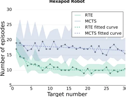
3.6 Hexapod Robot Results . . . 64
3.7 Conclusion and Discussion . . . 72
4 Flexible and Fast Model-Based Policy Search Using Black-Box Optimization 75 4.1 Introduction . . . 76 4.2 Problem Formulation . . . 78 4.3 Approach . . . 78 4.4 Experimental Setup . . . 83 4.5 Results . . . 85
4.6 Improving performance and computation times with empirical bootstrap and races . . . 94
CONTENTS 7
4.7 Handling sparse reward scenarios . . . 99
4.8 Conclusion and discussion . . . 104
5 Combining Model Identification and Gaussian Processes for Fast Learning 106 5.1 Introduction . . . 106
5.2 Problem Formulation . . . 108
5.3 Approach . . . 109
5.4 Experimental Results . . . 113
5.5 Conclusion and Discussion . . . 118
6 Collaborations: Bayesian Optimization for Micro-Data Re-inforcement Learning 120 6.1 Introduction . . . 121
6.2 Safety-aware Intelligent Trial-and-Error for Robot Damage Re-covery . . . 122
6.3 Alternating Optimization and Quadrature for Robust Control . 126 6.4 Bayesian Optimization with Automatic Prior Selection . . . 136
7 Discussion 148 7.1 Learning surrogate models . . . 148
7.2 Using simulators to improve learning . . . 152
7.3 Exploiting structured knowledge to improve learning . . . 153
7.4 Interplay between model-predictive control, planning and policy search . . . 156
7.5 Computation time . . . 158
8 Conclusion 160
Bibliography 164
List of Figures
2.1 Overview of possible strategies for Micro-Data Policy Search (MDPS) 19
3.1 Reset-free Trial-and-Error (RTE) algorithm . . . 49
3.2 Overview of Reset-free Trial-and-Error (RTE) algorithm . . . 52
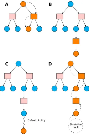
3.3 Overview of Monte Carlo Tree Search algorithm . . . 56
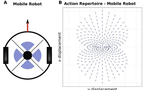
3.4 Mobile robot setup and repertoire . . . 60
3.5 Mobile robot task environment . . . 63
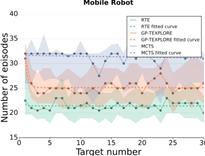
3.6 Comparison between RTE, GP-TEXPLORE and MCTS-based plan-ning — Differential drive robot simulation results . . . 64
3.7 Mobile robot detailed results . . . 65
3.8 Sample trajectories of RTE, GP-TEXPLORE and MCTS in the mobile robot task . . . 66
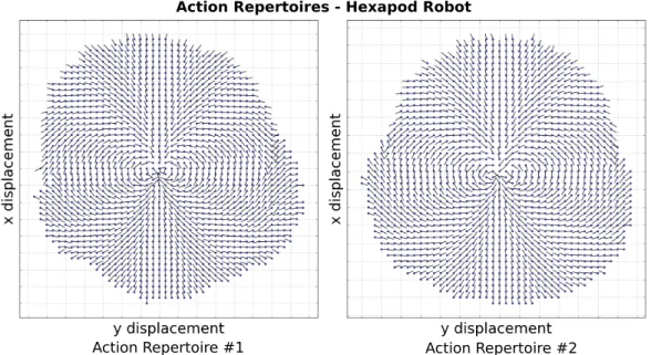
3.9 Hexapod locomotion task repertoires . . . 66
3.10 Comparison between RTE, GP-TEXPLORE and MCTS-based plan-ning — Hexapod robot simulation results. . . 67
3.11 Comparison between RTE, GP-TEXPLORE and MCTS-based plan-ning — Hexapod robot simulation distances . . . 68
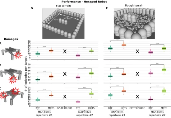
3.12 Hexapod locomotion detailed simulation results . . . 69
3.13 Sample trajectories of RTE, GP-TEXPLORE and MCTS in the simulated hexapod robot task . . . 70
3.14 Physical damaged hexapod robot . . . 71
3.15 Comparison between RTE and MCTS-based planning — Physical hexapod robot experiments . . . 71
3.16 Sample trajectories of RTE and MCTS in the physical hexapod robot task . . . 72
4.1 Illustration of CMA-ES. . . 80
4.2 Results for the noiseless pendulum task with the saturating reward (80 replicates) . . . 85
4.3 Timing for the the pendulum task with the saturating reward . . . 87
4.4 Results for the noisy pendulum task with the saturating reward (80 replicates) . . . 89
4.5 Results for the noisy pendulum task with the quadratic reward (20 replicates) . . . 90
4.6 Results for the noiseless cart-pole task with the saturating reward (80 replicates) . . . 91
List of Figures 9
4.7 Timing for the cart-pole task with the saturating reward . . . 92
4.8 Results for the noisy cart-pole task with the saturating reward (80 replicates) . . . 93
4.9 Results for the noisy cart-pole task with the quadratic reward (20 replicates) . . . 94
4.10 Manipulator task . . . 95
4.11 Illustration of racing with bootstrap . . . 96
4.12 Results for the very noisy pendulum task (20 replicates) . . . 97
4.13 Optimization time for the very noisy pendulum task (20 replicates) 98 4.14 Results for the deceptive pendulum swing-up task . . . 102
4.15 Results for the drawer opening task . . . 103
5.1 Hexapod locomotion task . . . 107
5.2 The pendubot system . . . 113
5.3 Results for the pendubot task (30 replicates of each scenario) — Tunable & Useful and Tunable priors . . . 114
5.4 Results for the pendubot task (30 replicates of each scenario) — Tunable & Misleading and Partially tunable priors . . . 116
5.5 Black-DROPS with GP-MI: Walking gait on a damaged hexapod . 117 5.6 Results for the physical hexapod locomotion task (5 replicates of each scenario) . . . 118
6.1 Overview of the safety-aware IT&E algorithm . . . 123
6.2 Comparison between IT&E, MO-IT&E and sIT&E . . . 125
6.3 Performance and learned configurations on the robotic arm joint breakage task. . . 133
6.4 Hexapod locomotion problem. . . 134
6.5 Experimental setup for TALOQ . . . 135
6.6 The 6-legged robot . . . 141
6.7 Comparison in simulation of MLEI with other acquisition functions 143 6.8 Comparison of MLEI with the standard EI with a single prior coming from a simulated undamaged robot . . . 146
List of Tables
3.1 Recovered locomotion capabilities - Mobile Robot Task . . . 63
3.2 Recovered locomotion capabilities - Hexapod Robot Task (Flat terrain scenarios) . . . 69
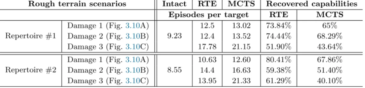
3.3 Recovered locomotion capabilities - Hexapod Robot Task (Rough terrain scenarios) . . . 70
4.1 Success Rates for Pendulum . . . 86
4.2 Success Rates for Cart-pole . . . 90
5.1 Actual system and priors for the pendubot task. . . 113
6.1 Evolution of the expected reward on the physical robot using TALOQ136
Chapter 1
Introduction
Aristotle may have been the first to describe how automated mechanical statues could replace slaves and reduce the burden of everyday labor1. Since then, numerous advances in physics, mechanical engineering, computer science and mathematics have allowed the wide deployment of automated systems and robots in our everyday life and especially inside factories. For example, FANUC has been operating a “lights out” factory for robots since 2001 (Null and
Caulfield, 2003) (a “lights out” factory is one where there are no light, no
humans and only robots operate inside it), iRobot has sold more than 8 million robot vacuums, and Amazon currently has more than 10 thousand autonomous mobile robots inside their semi-autonomous warehouses.
Although these robots operate autonomously, they still require humans to specify their tasks and supervise them. Ideally, we would imagine fully autonomous robots operating in various conditions and interacting with humans and the environment. Robots could operate in homes helping with the chores, learning and improving over time. Robots could autonomously design rescue plans and operate in post-disaster sites. Robots could also assist people working in the elderly services by providing physical assistance to elders. Autonomous cars could reduce the number of accidents and minimize the commute time. Overall, we currently have machines that can fulfill specific tasks very well, but none of the currently deployed robots are capable to adapt to truly unforeseen events and improve over time with experience.
Traditionally, robots have been studied under the rigid body dynamics theory and more specifically as chains (either open or closed) of rigid bodies (Murray, 1In his Politics (322BC, book 1, part 4), he says: There is only one condition in which we can imagine managers not needing subordinates, and masters not needing slaves. This condition would be that each instrument could do its own work, at the word of command or by intelligent anticipation, like the statues of Daedalus or the tripods made by Hephaestus, of which Homer relates that “Of their own motion they entered the conclave of Gods on Olympus”, as if a shuttle should weave of itself, and a plectrum should do its own harp playing. Original: εἰ γὰρ ἠδύνατο ἕκαστον τῶν ὀργάνων κελευσθὲν ἢ προαισθανόμενον ἀποτελεῖν τὸ αὑτοῦ ἔργον, ὥσπερ τὰ Δαιδάλου φασὶν ἢ τοὺς τοῦ ῾Ηφαίστου τρίποδας, οὕς φησιν ὁ ποιητὴς αὐτομάτους θεῖον δύεσθαι ἀγῶνα, οὕτως αἱ κερκίδες ἐκέρκιζον αὐταὶ καὶ τὰ πλῆκτρα ἐκιθάριζεν, οὐδὲν ἂν ἔδει οὔτε τοῖς ἀρχιτέκτοσιν ὑπηρετῶν οὔτε τοῖς δεσπόταις δούλων. 11
CHAPTER 1. INTRODUCTION 12
2017; Lynch and Park, 2017). This mathematical framework in conjunction
with advances in materials and actuators have allowed the development of reliable and robust control algorithms with impressive results (Rawlings and
Mayne, 2009; Krstic et al., 1995; Garcia et al., 1989; ˚Astr¨om, 2012). For
instance, modern manipulators can be controlled at 1KHz with millimeter precision (Kyriakopoulos and Saridis, 1988; Bischoff et al., 2011), humanoid robots can now walk reliably on flat terrain (Sellaouti et al.,2006;Mansard et al.,
2009) and even robustly perform choreographies under perturbations (Padois
et al., 2017;Nori et al.,2015). A few more noteworthy examples are the robots
of Boston Dynamics (a US robotics company), like Big Dog (Raibert et al.,
2008) and Atlas (Nelson et al.,2012;DARPA,2013), that are able to showcase locomotion abilities that are very life-like and robust to multiple real-world terrains like snow, grass and rocky roads in forests.
Although these approaches have provided very impressive results and could serve as the basis for more complicated or alternative approaches, the task specifications are usually hard-coded by the programmers or the designers; usually this is described in joint or end-effector acceleration, velocity or position profiles (i.e., joint or end-effector trajectories) (Kyriakopoulos and Saridis,1988). In addition, these approaches usually assume perfect knowledge of the system dynamics or very high frequency control loops that may be hard to acquire in practice. Overall, current robots are designed to achieve high-performance on specific tasks, but fail to perform when something unexpected happens (Atkeson
et al.,2016). In other words, the currently deployed robots are not designed to
adapt to unforeseen situations. This realization yields the need for alternative approaches for controlling robots inside a constantly changing world.
Getting inspiration from how animals and humans think and act, robots could also learn from experience and improve their skills over time. Learning by trial-and-error is one of the main challenges of Artificial Intelligence (AI) since its beginnings (Russell and Norvig,2016). Robotics and AI have a long standing, relationship with some notable results. For example, in 1984, Shakey the robot could autonomously navigate an indoor building and interact with voice commands (Nilsson, 1984); Ng et al. (2006) were able to use demonstrations from experts and learn models of the dynamics in order to successfully learn how to perform dynamic and complex maneuvers with a physical helicopter;Calinon
et al. (2007) were able to use a few demonstrations (i.e., 4 to 7) from an expert
in order to teach a humanoid robot to perform some simple manipulation tasks, like moving a chess pawn to a specified location.
The long-term vision of learning in robotics is to create autonomous and intelligent robots that can adapt in various situations, learn from their mistakes (that is, by trial-and-error), and require no human supervision. This is usually referred to as General Artificial Intelligence (GAI) (Legg and Hutter,2007) and has been one of the main long-term goals of all AI research. In practice, GAI has mostly been studied in the field of computer games with a few noteworthy results. The goal here is to create an algorithm that can learn how to play multiple and different games without any human intervention or reprogramming. For example, PathNet (Fernando et al., 2017) demonstrates transfer learning
CHAPTER 1. INTRODUCTION 13
capabilities between Atari games by using an evolutionary algorithm in order to select which parts of a neural network should be used for learning new tasks, and Elastic Weight Consolidation (Kirkpatrick et al.,2017) can learn multiple Atari games sequentially without catastrophic forgetting by protecting weights that are important for the previously learned tasks. In robotics, GAI has been mostly studied either theoretically or on simple tasks within the areas of evolutionary and developmental robotics (Oudeyer et al., 2007; Moulin-Frier
and Oudeyer, 2013;Schmidhuber, 2006).
Within the field of AI, Machine Learning (ML) (Michalski et al., 2013) has provided the most successful algorithms towards solving the challenge of GAI. ML uses statistical methods to enable computer systems to learn by trial-and-error, that is, to improve with more data without being explicitly programmed. We can split the ML algorithms into three main categories: (1) supervised learning (Russell and Norvig, 2016), (2) reinforcement learning (RL) (Sutton and Barto, 1998), and (3) unsupervised learning. In supervised learning, the system is presented with labeled samples (i.e., input with desired outputs given by an oracle) and the task is to learn a mapping (e.g., a function) from the input space to the output space. In reinforcement learning, the agent is given rewards (or punishments) as a feedback to its actions (and current state) in a possibly dynamic environment. In other words, the agent receives reinforcement signals when the actions it takes help towards solving the desired task(s). In unsupervised learning, no labels or reward signals are given to the system and the system has to discover the underlying or hidden structure of the data (e.g., clustering).
There is currently a renewed interest in machine learning and reinforcement learning thanks to recent advances in deep learning (LeCun et al., 2015). For example, deep convolutional neural networks have achieved extraordinary results in detection, segmentation and recognition of objects and regions in images (Vaillant et al.,1994;Lawrence et al.,1997;Cire¸sAn et al.,2012;Turaga
et al.,2010), especially in face recognition (Garcia and Delakis, 2004; Taigman
et al.,2014), and Deep RL agents can now learn to play many of the Atari 2600
games directly from pixels (Mnih et al., 2015, 2016), that is, without explicit feature engineering, and beat the world’s best players at Go and chess with minimal human knowledge (Silver et al., 2017b,a).
Unfortunately, these impressive results are difficult to transfer to robotics because the algorithms behind them are highly data-hungry: 4.4 million labeled faces were required by DeepFace to achieve the reported results (Taigman et al.,
2014), 4.8 million games were required to learn to play Go from scratch (Silver
et al., 2017b), 38 days of play (real time) for Atari 2600 games (Mnih et al.,
2015), and, for example, about 100 hours of simulation time (much more for real time) for a 9-DOF mannequin that learns to walk (Heess et al., 2017). By contrast, robots have to face the real world, which cannot be accelerated by GPUs nor parallelized on large clusters. And the real world will not become faster in a few years, contrary to computers so far (Moore’s law). In concrete terms, this means that most of the experiments that are successful in simulation cannot be replicated in the real world because they would take too much time
CHAPTER 1. INTRODUCTION 14
to be technically feasible.
What is more, online adaptation is much more useful when it is fast than when it requires hours — or worse, days — of trial-and-error. For instance, if a robot is stranded in a nuclear plant and has to discover a new way to use its arm to open a door; or if a walking robot encounters a new kind of terrain for which it is required to alter its gait; or if a humanoid robot falls, damages its knee, and needs to learn how to limp: in most cases, adaptation has to occur in a few minutes or within a dozen trials to be of any use.
The above requirement stems from the fact that robots are not only in-telligent agents, but they also have physical bodies that shape the way they
act (Pfeifer and Bongard, 2006). This essentially means that when a robot is
trying to complete a task, it is not an abstract agent, but rather a physical agent that interacts with a specific body with the environment. Rodney Brooks describes approaches that are based on this observation as “Nouvelle AI” or “Physically Grounded Methods” (Brooks, 1990), while others refer to them as “Embodied Cognition”. Pfeifer and Bongard (Pfeifer and Bongard, 2006) go even further and make the statement that “intelligence requires a body”, which implies that a disembodied agent (e.g., a computer program) cannot be intelligent.
In this thesis, we consider that robots, as embodied systems, are subject to the laws of physics (e.g., gravity, friction, energy supply, etc.) and thus cannot be considered as abstract intelligent agents. Consequently, it is of extreme importance to minimize the interaction time between the robot and the environment when using learning algorithms for robot control, as robots are bounded to their physical capabilities and limitations: for example, a mechanical motor has only a limited number of cycles before it dies and thus we cannot use the robot infinitely during the learning procedure.
By analogy with the word “big-data”, we refer to the challenge of learning by trial-and-error in a few minutes as “micro-data reinforcement learning” (Mouret,
2016). This concept is close to “data-efficient reinforcement learning” (
Deisen-roth et al., 2015, 2013), but we think it captures a slightly different meaning.
The main difference is that efficiency is a ratio between a cost and benefit, that is, data-efficiency is a ratio between a quantity of data and, for instance, the complexity of the task. In addition, efficiency is a relative term: a process is more efficient than another; it is not simply “efficient”2. In that sense, many deep learning algorithms are data-efficient because they require fewer trials than the previous generation, regardless of the fact that they might need millions of them. By contrast, we propose the terminology “micro-data learning” to represent an absolute value, not a relative one: how can a robot learn in a few minutes of interaction? or how can a robot learn in less than 20 trials3? Importantly, a micro-data algorithm might reduce the number of trials by
2In some rare cases, a process can be “optimally efficient”.
3It is challenging to put a precise limit for “micro-data learning” as each domain has different experimental constraints, this is why we will refer in this manuscript to “a few minutes”, a “a few trials” or a “handful of trials”. The commonly used word “big-data” has a similar “fuzzy” limit that depends on the exact domain.
CHAPTER 1. INTRODUCTION 15
incorporating appropriate prior knowledge. This does not necessarily make it more “data-efficient” than another algorithm that would use more trials but less prior knowledge: it simply makes them different because the two algorithms solve a different challenge.
The main objective of this thesis is to provide algorithms towards solving this “micro-data reinforcement learning” challenge by leveraging prior knowledge or building surrogate models. The overall goal of the proposed approaches is to minimize the interaction time between the robot and the environment required to solve the task at hand (i.e., minimize the operation time of the robot). We argue that this is the most appropriate metric to compare trial-and-error algorithms and we use it throughout this manuscript. Other metrics like the number of episodes or time-steps are very dependent on the specific task setups and can easily be “overfitted”.
Our main motivation is the application of reinforcement learning to robot damage recovery. In our opinion, this is an application that can justify learning in the robotics community, as there is presently no consensus about the best analytic way to recover from damages in robots. Nevertheless, we additionally provide examples of general adaptation (i.e., unforeseen situations that do not necessarily involve damage) and most of the algorithms presented do not have the explicit goal of solving this challenge, but rather the “micro-data reinforcement learning” challenge.
In the next chapter (chapter 2), we provide a review of policy search approaches (Deisenroth et al.,2013; Kober et al., 2013) that have the explicit goal of reducing the interaction time between the robot and the environment to a few seconds or minutes. Policy search methods learn parameters of a controller, called the policy, that maps sensor inputs to motor commands (e.g., velocities or torques). We will see that most published algorithms for micro-data policy search implement and sometimes combine two main strategies: leveraging prior knowledge and building surrogate models.
Prior knowledge can be incorporated either in the policy structure, the policy parameters or the dynamics model. In the first case, this knowledge comes from the traditional robotics literature and the methods use well defined policy structures in order to make the search problem easier. Some examples of well defined policy spaces are: dynamic movement primitives (Ijspeert et al.,
2013), finite-state automata (Calandra et al., 2015) or other hand-designed structures. In the second case, learning from demonstrations (Billard et al.,
2008;Kober and Peters,2009) or imitation learning has a long successful history
in robotics; in short, demonstrated trajectories provide initialization of the parameters of an expressive policy such that local search around them is enough to find high-performing solutions. Lastly, recent works (Chatzilygeroudis and
Mouret, 2018; Chatzilygeroudis et al., 2018b;Cutler and How, 2015; Saveriano
et al., 2017; Bongard et al., 2006; Zhu et al., 2018) showcase that taking
advantage of dynamics simulators or inaccurate simple dynamics models can help in reducing the amount of interaction time required to obtain an accurate model of the real-world environment.
CHAPTER 1. INTRODUCTION 16
and create models to help us make better decisions on what to try next. We can find two types of algorithms inside this strategy: (a) algorithms that learn a surrogate model of the expected return from a starting state distribution (Brochu et al., 2010; Shahriari et al., 2016), and (b) algorithms that learn the transition dynamics of the robot/environment (Deisenroth et al.,
2013; Chatzilygeroudis et al., 2018b). In the first case, the most promising
family of approaches is Bayesian optimization (BO) (Brochu et al., 2010;
Shahriari et al.,2016); BO is made of two main components: a surrogate model
of the expected return, and an acquisition function, which uses the model to define the utility of each point of the search space. In the second case, using probabilistic models, like Gaussian processes (GPs) (Rasmussen and Williams,
2006), and taking into account the uncertainty of the predictions in the policy search seems to be the most promising direction of research for model-based policy search (Deisenroth et al.,2013; Chatzilygeroudis et al.,2018b;Polydoros
and Nalpantidis, 2017).
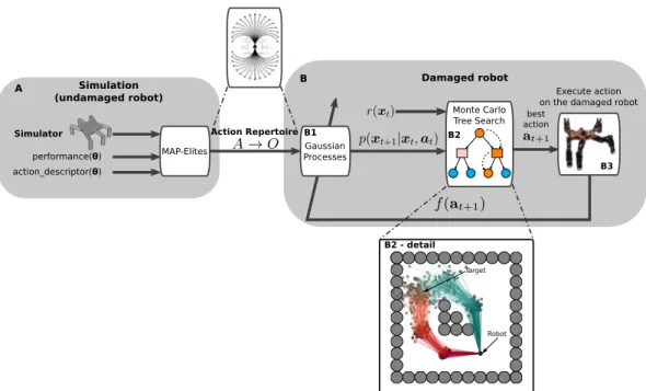
In chapter 3, we consider a robot damage recovery scenario, where a waypoint-controlled robot is damaged in an unknown way and needs to find novel gaits in order to reach the waypoints fixed by its operator. To tackle this challenge, we combine probabilistic modeling and planning with a repertoire of high-level actions produced using a dynamics simulator of the intact robot. In this work, we will show that evolutionary algorithms, and more precisely quality-diversity or illumination algorithms (Mouret and Clune, 2015; Pugh
et al.,2016), produce “creative priors” that can be beneficial when searching
for a compensating behavior. We propose a new algorithm, called “Reset-free Trial-and-Error” (RTE), and we evaluate it on a simulated wheeled robot, a simulated six-legged robot, and a physical six-legged walking robot that are damaged in several ways (e.g., a missing leg, a faulty motor, etc.) and whose objective is to reach a sequence of targets in an arena. Our experiments show that the robots can recover most of their locomotion abilities in an environment with obstacles, and without any human intervention.
In chapter4, we confirm the result of the PILCO papers (Deisenroth and
Rasmussen,2011;Deisenroth et al.,2015, 2013) that using probabilistic models
and taking into account the uncertainty of the prediction in the policy search is essential for effective model-based policy search (Deisenroth et al.,2015, 2013;
Kober et al., 2013; Sutton and Barto, 1998). We, also, go one step further
and showcase that combining the policy evaluation step with the optimization procedure can give us a more flexible, faster and modern implementation of model-based policy search algorithms. We propose a new model-based policy search algorithm, called Black-DROPS, and evaluate it on two standard benchmark tasks (i.e., inverted pendulum and cartpole swing-up) and a physical manipulator. Our results showcase that we can keep the low interaction times of analytical approaches like PILCO, but also speed-up the computation due to the parallelization properties of population-based optimizers like CMA-ES (Hansen
and Ostermeier, 2001).
In chapter 5, we combine dynamics simulators and Gaussian processes in order to scale up model-based policy search approaches to high-dimensional
CHAPTER 1. INTRODUCTION 17
robots. In particular, we introduce a new model learning procedure, called GP-MI, that combines model identification, black-box parameterized priors and Gaussian process regression. Overall, we argue that vanilla model-based policy search approaches are only practical in low-dimensional systems, but can be very powerful when combined with the appropriate prior knowledge and model learning procedure. Our results showcase that by combining Black-DROPS with GP-MI, we can learn to control a physical hexapod robot (48D state space, 18D action space) in less than one minute of interaction time.
In chapter 6, we discuss how safety constraints, robustness and multiple priors can be incorporated in a Bayesian optimization procedure towards solving the micro-data reinforcement learning challenge. More precisely, we first intro-duce sIT&E (Safety-aware Intelligent Trial & Error Algorithm) that extends the Intelligent Trial & Error algorithm to include safety criteria in the learning process; using this approach, a simulated damaged iCub humanoid robot (Nori
et al., 2015; Tsagarakis et al., 2007) is able to safely learn crawling behaviors
in less than 20 trials. We then propose ALOQ (ALternating Optimization and Quadrature) and TALOQ (Transferable ALOQ) aimed towards learning policies that are robust to rare events while being as sample efficient as possible. Using these approaches we learn robust policies using accurate and inaccurate simulators for a variety of systems (from simple simulated arms to a physical hexapod robot). Lastly, we introduce a new acquisition function for BO, called MLEI (Most Likely Expected Improvement), that effectively combines multiple sources of prior information in order to minimize the interaction time. Using MLEI a hexapod robot is able to find effective gaits in order to climb new types of stairs and adapt to unforeseen damages.
Before the conclusion of this manuscript (chapter 7), we discuss the main limitations of our proposed approaches and the main directions for future work. In this last chapter, we also highlight the interplay between planning, model-predictive control and policy search methods and discuss the main challenges that this new emerging field (micro-data reinforcement learning) faces.
Chapter 2
Background
The text of this chapter has been partially published in the following articles.
Articles:
• Chatzilygeroudis, K., Vassiliades, V., Stulp, F., Calinon, S. and Mouret, J.-B., 2018. A survey on policy search algorithms for learning robot controllers in a handful of trials. Under review in IEEE Transactions on Robotics (Chatzilygeroudis et al.,2018b).
Other contributors:
• Vassilis Vassiliades (Post-doc)
• Freek Stulp (Head of department at DLR) • Sylvain Calinon (Senior researcher at Idiap) • Jean-Baptiste Mouret (Thesis supervisor) Author contributions:
• KC and JBM organized the study. KC wrote the majority of the survey with improvements and suggestions by VV and JBM. FS and SC wrote most of section2.5.
2.1
Introduction
The most successful traditional RL methods typically learn an action-value function that the agent consults to select the best action from each state (i.e., one that maximizes long-term reward) (Sutton and Barto, 1998; Mnih et al.,
2015). These methods work well in discrete action spaces (and even better when combined with discrete state spaces)1, but robots are typically controlled with continuous inputs and outputs (see (Deisenroth et al., 2013;Kober et al.,
2013) for detailed discussions on the issues of classic RL methods in robotics). 1In Section2.4 we give a brief overview of approaches based on value or action-value functions for continuous control.
CHAPTER 2. BACKGROUND 19
priors models
dynamics policy expected return
model-based policy search Bayesian optimization
prior on dynamics prior on expected return
simulations, demonstrations, analytical models, experimenter's insights, ... system prior on parameters e.g., demonstra tions prior on structure
e.g., dynamic movem
ent prim
itives
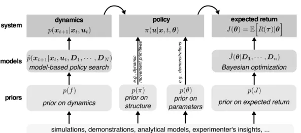
Figure 2.1: Overview of possible strategies for Micro-Data Policy Search (MDPS). The first strategy (bottom) is to leverage prior knowledge on the dynamics, on the policy parameters, on the structure of the policy, or on the expected return. A second strategy is to learn surrogate models of the dynamics or of the expected return; these models can also be initialized or guided by some prior knowledge.
As a result, the most promising approaches to RL for robot control do not rely on value functions; instead, they are policy search methods that learn parameters of a controller, called the policy, that maps sensor inputs to joint positions/torque (Deisenroth et al., 2013). These methods make it possible to use policies that are well-suited for robot control such as dynamic movement primitives (Ijspeert et al., 2003) or general-purpose neural networks (Levine
and Koltun, 2013). In direct policy search, the algorithms view learning as
an optimization problem that can be solved with gradient-based or black-box optimization algorithms (Stulp and Sigaud, 2013b). As they are not modeling the robot itself, these algorithms scale well with the dimensionality of the state space. They still encounter difficulties, however, as the number of parameters which define a policy, and thus the dimensionality of the search space, increases (Deisenroth et al.,2013). In model-based policy search, the algorithms typically alternate between learning a model of the robot and learning a policy using the learned model (Deisenroth et al., 2015; Chatzilygeroudis et al., 2017). As they optimize policies without interacting with the robot, these algorithms not only scale well with the number of parameters, but can also be very data efficient, requiring few trials on the robot itself to develop a policy. They do not scale well with the dimensionality of the state space, however, as the complexity of the dynamics tends to scale exponentially with the number of moving components.
In this chapter, we focus on policy search approaches that have the explicit goal of reducing the interaction time between the robot and the environment to a few seconds or minutes. Most published algorithms for micro-data policy search implement and sometimes combine two main strategies (Fig. 2.1): leveraging prior knowledge and building surrogate models.
CHAPTER 2. BACKGROUND 20
realistically known before learning and what is left to be learnt. For instance, some experiments assume that demonstrations can be provided, but that they are imperfect (Ng et al.,2006; Kober and Peters, 2009); some others assume that a damaged robot knows its model in its intact form, but not the damaged model (Cully et al., 2015; Pautrat et al., 2018; Chatzilygeroudis and Mouret,
2018). This knowledge can be introduced at different places, typically in the structure of the policy (e.g., dynamic movement primitives; DMPs) (Ijspeert
et al., 2003), in the reward function (e.g., reward shaping), or in the dynamical
model (Abbeel et al., 2006;Chatzilygeroudis and Mouret, 2018).
The second strategy is to create models from the data gathered during learning and utilize them to make better decisions about what to try next on the robot. We can further categorize these methods into (a) algorithms that learn a surrogate model of the expected return (i.e., long-term reward) from a starting state (Brochu et al., 2010; Shahriari et al., 2016); and (b) algorithms that learn models of the transition dynamics and/or the immediate reward function (e.g., learning a controller for inverted helicopter flight by first learning a model of the helicopter’s dynamics (Ng et al.,2006)). The two strategies — priors and surrogates — are often combined; for example, most works with a surrogate model impose a policy structure and some of them use prior information to shape the initial surrogate function, before acquiring any data.
The rest of the chapter is structured as follows. Section 2.2 presents the problem formulation for reinforcement learning. Section 2.3 provides a brief overview of value-function based approaches and Section 2.4 discusses the goals of policy search and presents briefly the most important direct policy search approaches. Section 2.5describes the work about priors on the policy structure and parameters. Section 2.6 provides an overview of the work on learning surrogate models of the expected return, with and without prior, while Section 2.7is focused on learning models of the dynamics and the immediate reward. Section 2.8 lists the few noteworthy approaches for micro-data policy search that do not fit well into the previous sections.
2.2
Problem formulation
We model the robots as discrete-time dynamical systems that can be described by Markovian transition probabilities of the form:
p(xt+1|xt, ut) (2.1)
with continuous-valued states x ∈ RE and controls u ∈ RF.
If we assume deterministic dynamics and Gaussian system noise, this equation is often written as:
xt+1 = f (xt, ut) + w (2.2)
Here, w is i.i.d. Gaussian system noise, and f is a function that describes the unknown transition dynamics.
CHAPTER 2. BACKGROUND 21
We assume that the system is controlled through a parameterized policy π(u|x, t, θ) that is followed for T steps, where θ are the policy parameters. Throughout the chapter we adopt the episode-based, fixed time-horizon for-mulations for clarity and pedagogical reasons, but also because most of the micro-data policy search approaches use this formulation.
In the general case, π(u|x, t, θ) outputs a distribution (e.g., a Gaussian) that is sampled in order to get the action to apply; i.e., we have stochastic policies. Most algorithms utilize policies that are not time-dependent (i.e., they drop t), but we include it here for completeness. Several algorithms use deterministic policies; a deterministic policy means that π(u|x, t, θ) ⇒ u = π(x, t|θ).
When following a particular policy from an initial state distribution p(x0),
the system’s states and actions jointly form trajectories τ = (x0, u0, x1, u1, . . . ,
xT), which are often also called rollouts or paths. We assume that a scalar
performance system exists, R(τ ), that evaluates the performance of the system given a trajectory τ . This long-term reward (or return) is defined as the sum of the immediate rewards along the trajectory τ :
R(τ ) = T −1 X t=0 rt+1 = T −1 X t=0 r(xt, ut, xt+1) (2.3)
where rt+1 = r(xt, ut, xt+1) ∈ R is the immediate reward of being in state xt
at time t, taking the action ut and reaching the state xt+1 at time t + 1.
We define the expected return J(θ) when following a policy πθ for t
time-steps as:
J(θ) = EhR(τ )|θi =
Z
R(τ )P (τ |θ) (2.4)
where P (τ |θ) is the distribution over trajectories τ for any given policy pa-rameters θ applied on the actual system:
P(τ |θ) | {z } trajectories for θ = p(x0) | {z } initial state Y t p(xt+1|xt, ut) | {z } transition dynamics π(ut|xt, t, θ) | {z } policy (2.5)
Value function An important concept in RL is the value function. It represents the expected return of a state when the system is controlled with policy πθ. It differs from the reward function which is immediate in nature,
as value functions account for the effect of future rewards, determining the long-term expected reward of a given state. The value of a state x0 under a
policy πθ is the expected return of the system starting in state x0 and following
policy πθ thereafter: Vπθ(x0) = E h R(τ )|θ, x0 i = Z R(τ )P (τ |θ, x0) (2.6)
CHAPTER 2. BACKGROUND 22
Q-function Similarly, the action-value function or Q-function, Qπθ(x, u), is defined as the expected return of a state and action pair when the system is controlled with policy πθ:
Qπθ(x0, u0) = E h R(τ )|θ, x0, u0 i (2.7)
2.3
Value-function approaches
The value-function based approaches attempt to estimate either Vπθ(x) or Qπθ(x, u). In the rest of this section, we will briefly discuss the main concepts and algorithms that fall into this category. Nevertheless, in this dissertation we mainly focus on policy search algorithms with the explicit goal of minimizing the interaction/learning time and thus we cover them in more detail.
Dynamic Programming-Based Methods In this category, the approaches assume that the state and action spaces are discrete2 and the transition proba-bilities and immediate reward function fully known. These algorithms basically utilize the Bellman equation (Bellman, 1957):
Vπθ(xt) = E h rt+ γVπθ(xt+1) i (2.8) Qπθ(xt, ut) = E h rt+ γQπθ(xt+1, ut+1) i (2.9) where γ ∈ [0, 1] is a factor that discounts future rewards.
The classical Dynamic Programming (DP) algorithms (Bellman, 1957;
Werbos, 1992;Sutton and Barto,1998) are not used a lot because of their need
of a known model of the environment and because of their big computational cost (especially as the state/action space increases). However, they are still very interesting as they define fundamental computational mechanisms that can be used as parts of other more complicated algorithms.
Temporal Difference Methods Temporal Difference (TD) methods can learn directly from interaction with the environment with no prior model, and use bootstrapping to improve the value- or action-value function from the current estimates. TD learning methods can either be on-policy or off-policy. In on-policy learning, we learn the value of the policy being carried out by the agent including the exploration steps. SARSA (Rummery and Niranjan,
1994; Sutton and Barto, 1998) is on-policy as it updates the Q-values using
the Q-value of the next state and the current policy’s action; i.e., it estimates the return for state-action pairs assuming that the current policy continues to be followed. Off-policy methods are more general: they learn the value of a different policy (which could be the optimal policy or not) independently of 2For continuous problems, one could discretize the spaces and operate in them, but this would, usually, result in a very big number of states and actions.
CHAPTER 2. BACKGROUND 23 Algorithm 1 Generic policy search algorithm
1: Apply initialization strategy using InitStrategy 2: Collect data, D0, with CollectStrategy
3: for n = 1 → Niter do
4: Learn models using LearnStrategy and Dn−1
5: Calculate θn+1 using UpdateStrategy
6: Apply policy πθn+1 on the system
7: Collect data, Dn, with CollectStrategy
8: end for
the agent’s actions. Q-learning (Watkins and Dayan, 1992; Sutton and Barto,
1998) updates the Q-values using the Q-value of the next state and the greedy action; i.e., it estimates the return for state-action pairs assuming a greedy policy would be followed, and is independent of the policy being currently followed. Hence, off-policy methods are able to update the estimated value (or action-value) functions using hypothetical actions, that have not actually been tried, whereas on-policy methods update value (or action-value) functions based strictly on experience.
2.4
Policy Search
The objective of a policy search algorithm is to find the parameters θ∗ that
maximize the expected return J(θ) when following the policy πθ∗: θ∗ = argmax
θ
J(θ) (2.10)
Most policy search algorithms can be described with a generic algorithm (Algo.1) and they: (1) start with an initialization strategy (InitStrategy), for instance using random actions, and (2) collect data from the robot (Collect Strategy), for instance the states at each discrete time-steps or the reward at the end of the episode; they then (3) enter a loop (for Niter iterations) that
alternates between learning one or more models (LearnStrategy) with the data acquired so far, and selecting the next policy πθ∗ to try on the robot (UpdateStrategy).
This generic outline allows us to describe direct (e.g., policy gradient algorithms (Sutton et al., 2000)), surrogate-based (e.g., Bayesian optimiza-tion (Brochu et al., 2010)) and model-based policy search algorithms, where each algorithm implements in a different way each of InitStrategy, Col-lectStrategy, LearnStrategy and UpdateStrategy. We will also see that we can also fit policy search algorithms that utilize priors; coming from simulators, demonstrations or any other source.
To better understand how policy search is performed, let’s use a gradient-free optimizer (UpdateStrategy) and learn directly on the system (i.e., LearnStrategy = ∅). This type of algorithms falls in the category of model-free or direct policy search algorithms (Sutton and Barto, 1998; Kohl and
CHAPTER 2. BACKGROUND 24 Algorithm 2 Gradient-free direct policy search algorithm
1: procedure InitStrategy 2: Select θ0 randomly
3: end procedure
4: procedure CollectStrategy 5: Collect samples of the form (θ,
PN i R(τ )i
N ) = (θ, ˜Jθ) by running policy
πθ N times.
6: end procedure
Stone,2004). InitStrategy can be defined as randomly choosing some policy
parameters, θ0 (Algo. 2), and CollectStrategy collects samples of the form
(θ,
PN i R(τ )i
N ) by running N times the policy πθ. We execute the same policy
multiple times because we are interested in approximating the expected return (Eq. (2.3)). ˜Jθ =
PN i R(τ )i
N is then used as the value for the sample θ in a regular
optimization loop that tries to maximize it (i.e., the UpdateStrategy is optimizer-dependent).
This straightforward approach to policy search typically requires a large amount of interaction time with the system to find a high-performing solu-tion (Sutton and Barto, 1998). The objective of the present chapter is to describe algorithms that require several orders of magnitude less interaction time by leveraging priors and models.
In the rest of this section, we will briefly discuss the main concepts, formula-tions and algorithms that fall into the traditional direct policy search category. The approaches in this caterogy assume no prior knowledge of the system or the reward function and try to directly optimize the policy parameters on the real system (Kohl and Stone, 2004). As a result, these algorithms suffer from data-inefficiency, but nevertheless are important as they can be part of other more data-efficient approaches (e.g., as an initialization or an optimizer). In this manuscript we focus mainly on published ideas that explicitly try to drastically reduce the interaction time between the robot and the environment (we refer the reader to (Sigaud and Stulp, 2018) for a recent review of policy
search for continuous control).
2.4.1
Policy Gradient Algorithms
Sutton and Barto (1998) describe “Generalized Policy Iteration” (GPI) as
the process that consists of two interacting parts, one pushing the value function (or the Q-function) to be consistent with the best current policy (policy evaluation), and a second one that aims to improve the policy greedily using the current value function (policy improvement). In the classical policy iteration formulation (Sutton and Barto, 1998), these two processes strictly alternate; i.e., one happens exactly after the other has finished. Nevertheless, in more modern and asynchronous methods (Mnih et al., 2016), the policy evaluation and improvement steps can be interleaved at a finer grain. As long
CHAPTER 2. BACKGROUND 25
as both steps update all states, the result is typically the same-convergence to the optimal value function and an optimal policy (Sutton and Barto, 1998). A lot of reinforcement learning algorithms can be described using the GPI formalization and most of the policy gradient algorithms fall under it. It is also important to note that all approaches that fall under GPI (e.g., actor-critic methods) can also be seen as value-function based approaches. Nevertheless, we include them in the policy search section as the most successful policy gradient approaches do utilize some learned approximation of the value- or action-value function.
Actor-Critic Actor critic methods (Konda and Tsitsiklis,2000) fall under the GPI formulation and they, naturally, consist of two parts. The actor that adjusts the parameters θ of the policy by utilizing some policy gradient. And the critic that estimates the action-value function ˆQπ(x
t,ut) = Qπ(xt,ut) with
an appropriate policy evaluation method, e.g., temporal-difference learning. Stochastic Policy Gradients Policy gradient algorithms are the most popular class of continuous action reinforcement learning algorithms (Degris
et al.,2012; Silver et al., 2014; Ciosek and Whiteson, 2018a; Schulman et al.,
2015; Lillicrap et al., 2016; Zimmer et al., 2016). The overall idea is to adjust
the policy parameters θ in the direction of the performance gradient ∇θJ(θ).
Computing this gradient analytically is not possible, as the state distributions under every policy parameters and the real action-value function Q(x, u) should be known. To make this computation efficient and practical, most algorithms utilize the results of the stochastic policy gradient theorem (SPG) (Sutton et al.,
2000): ∇θJ(θ) = Z P(τ |θ) Z ∇θπ(u|x, θ)Qπ(x, u)dxdu = Eh T −1 X t=0 ∇θlogπ(ut|xt, θ)Qπ(xt,ut) i (2.11) The most interesting part of the policy gradient theorem (apart from its simplicity) is that despite the fact that the distribution over trajectories P (τ |θ) depends on the policy parameters θ, the policy gradient does not depend on the trajectory distribution. This result has very important practical value, as the computation of the policy gradient is reduced to a simple expectation. However, the stochastic policy gradient theorem requires that the policies are stochastic.
Deterministic Policy Gradients Silver et al. (2014) introduced the deterministic policy gradient theorem (DPG) that adapts the SPG theorem for deterministic policies:
CHAPTER 2. BACKGROUND 26 ∇θJ(θ) = Z P(τ |θ)∇uQπ(x, u = π(x|θ))dx = Eh T −1 X t=0 ∇θlogπ(xt|θ)∇utQ π (xt,ut= π(xt|θ)) i (2.12) They also showed that the DPG theorem is a limiting case of the SPG theorem. This is important because it shows that the familiar machinery of policy gradients, for example compatible function approximation (Sutton et al.,
2000), natural gradients(Kakade, 2002), actor-critic (Konda and Tsitsiklis,
2000), or episodic/batch methods, is also applicable to deterministic policy gradients.
Expected Policy Gradients Recently, Ciosek and Whiteson (2018a,b), taking inspiration from expected SARSA (Sutton and Barto,1998; Van Seijen
et al., 2009), introduced expected policy gradients (EPG) that unifies the SPG
and DPG theorems and shows improved performance on several benchmarks. Their main contribution is to restate the Eq. (2.11) as follows:
∇θJ(θ) = Z P(τ |θ) Z ∇θπ(u|x, θ)Qπ(x, u)dxdu = Z P(τ |θ)IQ π(x)dx = Eh T −1 X t=0 IπQ(xt) i (2.13) This formulation makes explicit that one step in estimating the gradient is to evaluate an integral. The key insight of EPG is that given a state xt, IπQ(xt)
can be fully expressed with known quantities. Consequently, IQ
π(xt) can be
analytically computed or approximated by Monte Carlo quadrature in cases where the integral is not possible to compute.
In their paper, Ciosek and Whiteson (2018b) formulate the General Policy Gradient Theorem that unifies both SPG and DPG theorems. In particular,
they show that the choice between a deterministic or a stochastic policy is fundamentally a choice of the quadrature method for approximating IQ
π (xt).
One important conclusion of their work is that the success of DPG over SPG should not be attributed to a fundamental issue of stochastic policies, but to superior (easier) quadrature method. Thanks to EPG, a deterministic policy is no longer required to obtain a method with low variance.
CHAPTER 2. BACKGROUND 27
2.5
Using priors on the policy parameters or
representation
When designing the policy π(u|x, t, θ), the key design choices are what the space of θ is, and how it maps states to actions. This design is guided by a trade-off between having a representation that is expressive, and one that provides a space that is efficiently searchable3.
Expressiveness can be defined in terms of the optimal policy π∗
ζ. For a given
task ζ, there is theoretically always at least one optimal policy π∗
ζ. Here, we
drop θ to express that we do not mean a specific representation parameterized by θ. Rather π∗
ζ emphasizes that there is some policy (with some representation,
perhaps unknown to us) that cannot be outperformed by any other policy (whatever its representation). We use Jζ(πζ∗) to denote this highest possible
expected reward.
A parameterized policy πθ should be expressive enough to represent this
optimal policy π∗
ζ (or at least come close), i.e.,
Jζ(πζ∗) − max
θ Jζ(θ) < δ, (2.14)
where δ is some acceptable margin of suboptimality. Note that absolute optimality is rarely required in robotics; in many everyday applications, small tracking errors may be acceptable, and the quadratic command cost needs not be the absolute minimum.
On the other hand, the policy representation should be such that it is easy (or at least feasible) to find θ∗, i.e., it should be efficiently searchable4. In
general, smaller values of dim(θ) lead to more efficiently searchable spaces. In the following subsections, we describe several common policy repre-sentations which make different trade-offs between expressiveness and being efficiently searchable.
2.5.1
Hand-designed policies
One approach to reducing the policy parameter space is to hand-tailor it to the task ζ to be solved. In (Fidelman and Stone, 2004), for instance, a policy for ball acquisition is designed. The resulting policy only has only four parameters, i.e., dim(θ) is 4. This low-dimensional policy parameter space is easily searched, and only 672 trials are required to optimize the policy. Thus, prior knowledge is used to find a compact representation, and policy search is used to find the optimal θ∗ for this representation.
3Freek Stulp and Sylvain Calinon greatly contributed in this section (Chatzilygeroudis
et al.,2018b).
4Analogously, the universal approximation theorem states that a feedforward network with single hidden layer suffices to represent any continuous function, but it does not imply that the function is learnable from data.
CHAPTER 2. BACKGROUND 28
One disadvantage of limiting dim(θ) to a very low dimensionality is that δ may become quite large, and we have no estimate of how much more the reward could have been optimized with a more expressive policy representation. Another disadvantage is that the representation is very specific to the task ζ for which it was designed. Thus, such a policy cannot be reused to learn other tasks. It then greatly limits the transfer learning capabilities of the approaches, since the learned policy can hardly be re-used for any other task.
2.5.2
Policies as function approximators
Ideally, our policy representation Θ is expressive enough so that we can apply it to many different tasks, i.e.,
argmin Θ N X n=1 Jζn(π ∗ ζn) − maxθ Jζn(θ), with θ ∈ Θ, (2.15) i.e., over a set of tasks, we minimize the sum of differences between the theoretically optimal policy π∗ for each task, and the optimal policy given the
representation πθ for each task5.
Two examples of such generally applicable policy representations are linear policies (2.16), radial basis function networks (2.17), or neural networks, namely
πθ(x) = θ|ψ(x) (2.16)
πθ(x) = w|ψθ(x). (2.17)
These more general policies can be used for many tasks (Guenter et al.,2007;
Kober et al., 2013). However, prior knowledge is still required to determine the
appropriate number of basis functions and their shape. Again, a lower number of basis functions will usually lead to more efficient learning, but less expressive policies and thus potentially higher δ.
One advantage of using a function approximator is that programming by demonstration can often be used to determine an initial policy. The initial parameters θ are obtained through supervised learning, by providing the demonstration as training data (xi, ui)i=1:N. This is discussed in more detail
in Section 2.5.6
The function approximator can be used to generate a single estimate (corresponding to a first order moment in statistics), but it can also be extended to higher order moments. Typically, extending it to second order moments allows the system to get information about the variations that we can exploit to fulfill a task, as well as the synergies between the different policy parameters in the form of covariances. This is typically more expensive to learn—or it requires multiple demonstrations (Matsubara et al., 2011)—but the learned representation can typically be more expressive, facilitating adaptation and generalization.
5Note that this optimization is never actually performed. It is a mathematical description of what the policy representation designer is implicitly aiming for.
CHAPTER 2. BACKGROUND 29
2.5.3
Dynamical Movement Primitives
Dynamical Movement Primitives (DMPs) combine the generality of function approximators with the advantages of dynamical systems, such as robustness towards perturbations and convergence guarantees (Ijspeert et al.,2013,2002). DMPs limit the expressiveness of the policy to typical classes of tasks in robotics, such as point-to-point movements (‘discrete DMPs’) or repetitive movements (‘rythmic DMPs’).
Discrete DMPs are summarized in Eq.2.18. The canonical system represents the movement phase s, which starts at 1, and converges to 0 over time. The transformation systems combines a spring-damper system with a function approximator fθ, which, when integrated, generates accelerations ¨y.
Multi-dimensional DMPs are achieved by coupling multiple transformation systems with one canonical system. The vector y typically represents the end-effector pose or the joint angles.
As the spring-damper system converges to yg, and s (and thus s f θ(s))
converges to 0, the overall system y is guaranteed to converge to yg. We have:
ω¨y= α(β(yg− y) − ˙y) | {z } Spring-damper system + s fθ(s) | {z } Forcing term . (Transf.) (2.18) ω˙s = −αss. (Canonical) (2.19)
This facilitates learning, because, whatever parameterization θ of the func-tion approximator we choose, a discrete DMP is guaranteed to converge towards a goal yg. Similarly, a rhythmic DMP will always generate a repetitive motion,
independent of the values in θ. The movement can be made slower or faster by changing the time constant ω.
Another advantage of DMPs is that only one function approximator is learned for each dimension of the DMP, and that the input of each function approximator is the phase variable s, which is always 1D. Thus, whereas the overall DMP closes the loop on the state y, the part of the DMP that is learned (fθ(s)) is an open-loop system. This greatly facilitates learning, and simple
black-box optimization algorithms have been shown to outperform state-of-the-art RL algorithms for such policies (Stulp and Sigaud, 2013a). Approaches for learning the goal yg of a discrete movement have also been proposed (Stulp
et al., 2012). Since the goal is constant throughout the movement, few trials
are required to learn it.
The optimal parameters θ∗ for a certain DMP are specific to one specific
task ζ. Task-parameterized (dynamical) motion primitives aim at generalizing them to variations of a task, which are described with the task parameter vector q (e.g., the 3D pose to place an object on a table (Stulp et al., 2013)). Learning a motion primitive that is optimal for all variations of a task (i.e., all q within a range) is much more challenging, because the curse of dimensionality applies to the task parameter vector q just as it does for the state vector x in reinforcement learning. Task-parameterized representations based on the use of multiple coordinate systems have been developed to cope with this curse of