HAL Id: tel-00755106
https://tel.archives-ouvertes.fr/tel-00755106
Submitted on 20 Nov 2012HAL is a multi-disciplinary open access archive for the deposit and dissemination of sci-entific research documents, whether they are pub-lished or not. The documents may come from teaching and research institutions in France or abroad, or from public or private research centers.
L’archive ouverte pluridisciplinaire HAL, est destinée au dépôt et à la diffusion de documents scientifiques de niveau recherche, publiés ou non, émanant des établissements d’enseignement et de recherche français ou étrangers, des laboratoires publics ou privés.
Individualisation of spectral cues for applications in
virtual auditory space: study of inter-subject differences
in head-related transfer functions using perceptual
judgements from listening tests
David Schönstein
To cite this version:
David Schönstein. Individualisation of spectral cues for applications in virtual auditory space: study of inter-subject differences in head-related transfer functions using perceptual judgements from listening tests. Acoustics [physics.class-ph]. Université Pierre et Marie Curie - Paris VI, 2012. English. �tel-00755106�
THÈSE DE DOCTORAT DE L’UNIVERSITÉ PIERRE ET MARIE CURIE Spécialité
SMAER Présentée par David Schönstein Pour obtenir le grade de
DOCTEUR de l’UNIVERSITÉ PIERRE ET MARIE CURIE
I N D I V I D U A L I S AT I O N O F S P E C T R A L C U E S F O R A P P L I C AT I O N S I N V I R T U A L A U D I T O R Y S PA C E : S T U D Y O F I N T E R - S U B J E C T D I F F E R E N C E S I N H E A D - R E L AT E D T R A N S F E R F U N C T I O N S U S I N G P E R C E P T U A L J U D G E M E N T S F R O M L I S T E N I N G T E S T S L’ I N D I V I D U A L I S AT I O N D E S I N D I C E S S P E C T R A U X P O U R L A S PAT I A L I S AT I O N A C O U S T I Q U E : É T U D E P E R C E P T I V E D E L A VA R I A B I L I T É I N T E R - I N D I V I D U E L L E D A N S L E S F O N C T I O N S D E T R A N S F E R T R E L AT I V E S À L A T Ê T E soutenue le 12 septembre 2012 devant le jury composé de :
Sabine Meunier Chargé de recherche CNRS, rapporteur Gaël Richard Chargé de recherche CNRS, rapporteur Brian Katz Chargé de recherche CNRS, HDR, directeur de thèse
Christophe d’Alessandro Directeur de Recherche CNRS, co-directeur de thèse Jean-Luc Zarader Professeur UPMC, examinateur
A B S T R A C T
The human auditory system has evolved to seamlessly interpret sounds from our environment. As the mechanisms underpinning our ability to accurately determine the nature and location of sound sources in space have become better understood, we have been able to apply this knowledge to technolo-gies that are of benefit to us. One of these technolotechnolo-gies is the ability to gener-ate compelling auditory illusions, or a Virtual Auditory Space (VAS). Despite a large emphasis in the past on virtual reality for vision, VASand its effec-tiveness in generating a compelling illusion, is now a field of research that is growing along with the many applications of the technology.
The theory behind how the illusion of a virtual sound source is created is in essence quite simple, and determined by the fact that the auditory system has all the information required to correctly interpret a sound source in space embedded in the sound waves that reach the auditory periphery at the level of the tympanic membrane inside the ear canal. Any number of different and competing sound sources can be in a sense smeared onto the basilar membrane and the auditory system is able to extract the most salient cues at the time in order to stream and interpret the auditory scene, as detailed in chapter 2. Thus, in order to provide a compelling illusion of sound sources in space all one has to do is reproduce the exact same signal to the auditory system as if sounds were originating from the desired location. This can be achieved by either using speakers or headphones; the latter being the focus of this body of work. One can imagine the simplest case in which small microphones are placed inside the ear canal and record the signal from a sound source in space, and then this recorded signal is played back to the same listener over headphones, adjusted to the correct level and placed at the exact location of where the microphones were. In this scenario the listener would perceive the sound source as if it originated at the location at a distance, instead of originating from the headphones, as the exact same acoustic information is being presented to the auditory system. The task of rendering any monophonic signal in VAS, known as binaural synthesis, is more complicated as detailed in chapter3.
The applications of binaural synthesis are far reaching given that it allows any signal to be virtually positioned in space when presented to the listener over headphones. One helpful use of binaural synthesis is for people who are hearing impaired and require hearing aids. The hearing impaired have difficulty in environments where many people are talking at the same time. A standard hearing aid will simply amplify all talkers and not provide infor-mation on the sound source location, which becomes almost impossible for the listener to understand since one of the most important ways the auditory system streams different sound sources, and is subsequently able to focus at-tention on one talker for example, is by using the sound source location as a cue. A hearing aid that can produce a binaural synthesis, providing cues
to sound source location, along with an amplification of the signal, could al-low for improved intelligibility in multi-talker environments. There remain however limitations to this technology for the hearing impaired as aids are often characterised by a reduced sensitivity for frequencies that are crucial for locating sound sources.
Another application of binaural synthesis, geared towards the general pub-lic, is the generation of immersive auditory experiences for movies and video games. This is akin to three-dimensional visual effects being used in cinemas today and acts as an augmentation of the different senses in order to make the experience more realistic and emotionally engaging. The technology of binaural synthesis has also been adopted by pilots of aeroplanes as an ad-ditional aid for negotiating the large amount of feedback from the console during a flight. A virtual sound source can be an indicator of elevation or pitch of an aeroplane as the sound is displaced above or below the listener’s head.
While the many applications of binaural synthesis are still emerging, stud-ies are still exploring the perceptually salient cues used by the auditory sys-tem in order to effectively interpret an auditory scene. A better understand-ing of how these mechanisms work will enable an improved experience for listeners in terms of producing a high fidelity rendering in VAS. One of the aspects of how sounds are perceived by the auditory system that researchers have isolated as being a critical component to the production of a realistic binaural synthesis, is the way in which sound sources are filtered by the human head and body, and in particular the outer ear, known as the Head-Related Transfer Function (HRTF). Embedded in the acoustic filtering effects of a listener’s morphology, represented by the HRTF, are cues that help
re-solve any ambiguity relating to the nature and location of a sound source in space, as detailed in chapter4.
The HRTF has been shown to be linked to the asymmetric shape of the
ear, or pinna, in ways that produce acoustic signatures to sound source lo-cation. Given that the shape of the ear varies from listener to listener, the way in which our auditory system is tuned to HRTFs also varies from
lis-tener to lislis-tener. These differences necessitate the use of what is known as individualisedHRTFs; theHRTFsthemselves are specific to the morphology of the listener (see chapter 5). Here in lies the difficulty in providing binaural synthesis as a technology to the masses; the task of acquiring HRTFs for a particular listener is in fact expensive and laborious. Whilst there are other factors that have an impact on the fidelity of a rendering in VAS, such as the headphones used and compensating for the way in which the headphone impacts the HRTF (a study performed in chapter 6), the problem of provid-ing some form of individualised HRTF for binaural synthesis stands as the major roadblock to making the technology more amenable to the consumer market. Arkamys, the company that has funded this research, was drawn to such a personalised audio experience in their pursuit to provide the highest quality digital audio solutions in the consumer electronics industry.
The pursuit of an elegant solution to HRTF individualisation has been evolving for some time with a range of different approaches available. One
difficulty in finding the best solution, is the question of what constitutes an effective rendering inVASand how to measure and quantify it? The majority of studies have looked at whether listeners are able to accurately determine the position of virtual sound sources, also known as localisation accuracy, as a measure of the quality of a binaural synthesis. The quantification of local-isation accuracy is done by measuring the disparity between the perceived and true location of a virtual sound source. This disparity measure was used in the current body of work in chapter6for testing different types of head-phones. In reality, localisation accuracy is only one aspect of what makes an effective binaural synthesis, and measuring localisation errors only one way of quantifying the effectiveness. Qualities such as the realism and nat-uralness of the illusion, the coherence of the auditory image, and whether the sound is perceived at the desired distance or inside the head, are as important as localisation, depending on the application of the technology. The concept of measuring the quality of a binaural synthesis, and quantify-ing it usquantify-ing metrics other than localisation errors, was explored in chapter7 via the use of listening tests. The ability of subjects to be able to make con-sistent perceptual judgements of a binaural synthesis using differentHRTFs
and listening tests was studied and considered an important precursor to any conclusions drawn with respect to a particular solution to theHRTF indi-vidualisation issue.
Once the perceptual limits of subjects in this context was understood to some degree, a study was performed, as described in chapter8, in order to build on what we know about the most perceptually salient components of theHRTF. An important aspect of this study was to provide a method for de-termining the best way to describe the differences inHRTFsbetween listeners
based on a perceptual validation. In being able to characterise the percep-tual differences betweenHRTFs, we are a step closer to understanding what it is about a rendering inVASthat makes it suitable for a particular listener,
and providing an individualised or personalisedHRTF. Of the many different approaches to producing individualisedHRTFsthat are explored in the litera-ture, the current body of work focused on a technique in which anHRTFwas
selected for a particular listener from a large database ofHRTFsobtained for many different listeners. In order to perform thisHRTF selection and avoid the costly procedure of obtainingHRTFsfrom the listener directly, the link
be-tween the subjects’ morphology andHRTFsin the database was tested using dimensions of the listener’s ear, or pinna, as detailed in chapter9.
R É S U M É
Le système auditif humain a évolué de façon à pourvoir interpréter efficace-ment les sons de notre environneefficace-ment. Grâce une meilleure compréhension de notre capacité à déterminer avec précision la nature et la position des sources sonores, nous sommes en mesure d’appliquer ces connaissances à des technologies bénéfiques pour l’homme. L’une de ces technologies est la capacité à générer des illusions auditives convaincantes, ou sources sonores
virtuelles. Malgré une importante concentration de la recherche sur les illu-sions virtuelles dans le domaine de la vision, les espaces acoustiques virtuels, ou Virtual Auditory Space (VAS) en anglais, sont désormais au cœur des recherches actuelles et ce nouveau domaine développe de nombreuses applications en lien avec cette technologie.
La théorie derrière la manière dont se crée l’illusion d’une source sonore virtuelle est en réalité assez simple. L’illusion se crée du fait que le système auditif dispose de toutes les informations nécessaires pour interpréter cor-rectement une source sonore dans l’espace, contenues dans les ondes sonores présentes au niveau de la membrane du tympan, à l’intérieur du conduit auditif. N’importe quel nombre de sources sonores différentes et concur-rentes peuvent être dans un sens plaquées contre la membrane basilaire, et le système auditif est alors capable d’en extraire les signaux les plus sail-lants à chaque moment afin de diffuser et interpréter la scène sonore, comme l’explique le chapitre 2. Ainsi, afin de fournir une illusion convaincante de source sonore dans l’espace, il suffit de reproduire un signal sonore de façon à ce que le système auditif l’interprète comme s’il provenait réellement de l’endroit désiré. Ceci peut être réalisé en utilisant des haut-parleurs ou un casque audio ; la transmission via casque, plus précisément, sera l’objet de la recherche présentée ici. Il est facile d’imaginer une expérience assez sim-ple où de minuscules microphones seraient placés à l’intérieur du conduit auditif afin d’enregistrer le signal d’une source sonore réelle. Le même sig-nal serait ensuite transmis au même sujet via le casque audio, correctement ajusté au bon niveau et placé à l’endroit exact où étaient les microphones. Dans ce scénario, le sujet percevrait le signal sonore comme s’il émanait d’une source située à une certaine distance et non pas provenant du casque audio en lui même puisque la même information sonore est présentée au système auditif. La tâche de transformer un signal monophonique en VAS, connue sous le nom de synthèse binaurale, est plus compliquée et est ex-pliquée en détail dans le chapitre3.
On trouve de nombreuses applications de la synthèse binaurale liées au fait qu’elle permet de présenter à un auditeur, via une écoute au casque, n’importe quel signal virtuellement positionné dans l’espace. Cette applica-tion se révèle notamment très utile pour les personnes souffrant d’une dé-ficience auditive nécessitant une prothèse afin de pallier aux difficultés ren-contrées dans des environnements où plusieurs personnes parlent en même temps. Une prothèse auditive standard se contente d’amplifier les sons émis par tous les locuteurs et ne fourni pas d’indications quant à la localisation de la source sonore, rendant quasiment impossible pour l’auditeur de savoir d’où provient le bruit. Or le système auditif fonctionne de telle façon que la localisation de la source sonore est utilisée comme repère afin de séparer les différentes sources sonores et se concentrer, par exemple, sur une per-sonne qui parle. Une prothèse auditive utilisant la synthèse binaurale qui pourrait procurer une information sur la position de la source sonore, tout en amplifiant les signaux sonores, pourrait alors améliorer l’intelligibilité de façon significative dans les environnements comprenant plusieurs locuteurs. Cette technologie a néanmoins ses limites puisque les prothèses utilisées par
les malentendants sont souvent caractérisées par une sensibilité réduite aux fréquences qui sont cruciales pour la localisation des sources sonores.
Une autre application de la synthèse binaurale, orientée vers le grand public cette fois, est la possibilité d’une immersion auditive totale dans les films ou jeux vidéo. Ceci s’apparente aux effets tridimensionnels utilisés au cinéma aujourd’hui afin de rendre l’expérience cinématographique plus réal-iste et plus touchante émotionnellement pour le public. La technologie de la synthèse binaurale a également été adoptée par les pilotes d’avion comme une aide supplémentaire permettant de mieux interpréter et gérer la quantité d’informations transmises par la console lors d’un vol. Une source sonore virtuelle peut être alors un indicateur de variation d’altitude ou de tangage d’un avion en générant une source sonore virtuelle de façon à ce qu’elle soit perçue comme au dessus ou en dessous de l’auditeur.
Alors que les nombreuses applications de la synthèse binaurale sont en en-core un domaine en pleine émergence, des études explorent actuellement les indices perceptivement saillants utilisé par le système auditif afin d’interpréter la source sonore. Une meilleure compréhension du fonctionnement de ces mécanismes permettrait une amélioration d’écoute pour les auditeurs en terme de production d’un rendu de grande fidélité enVAS. Un des aspects de la perception des sons par le système auditif, identifié comme essentiel à la synthèse binaurale par les chercheurs, est la manière dont les sources sonores sont filtrées par la tête et le corps humain, notamment l’oreille ex-terne, connue sous le nom de fonctions de transfert acoustique ou Head-Related Transfer Function (HRTF) en anglais. On trouve des indices concernant la nature et la position d’une source sonore dans l’espace, représentés par les HRTFs, dans les effets acoustiques de filtrage liée à la morphologie de
l’auditeur, comme l’explique en détails le chapitre4.
Il a été prouvé que lesHRTFssont liées à la forme asymétrique de l’oreille, ou du pavillon, de façon à produire des signatures acoustiques de la posi-tion de la source sonore. Etant donné que la morphologie de l’oreille varie d’un auditeur à un autre, la façon dont notre système auditif s’accorde avec lesHRTFsvarie elle aussi. Ces différences nécessitent l’utilisation de ce qu’on
appelle desHRTFsindividualisés puisque lesHRTFssont spécifiques à la mor-phologie de l’auditeur comme le détaille le chapitre 5. Ceci représente le plus grand défi rencontré par l’application de la synthèse binaurale pour une écoute destinée au grand public, la tâche de produire unHRTF pour un auditeur spécifique étant coûteuse et laborieuse. De nombreux facteurs influ-encent la qualité d’un rendu enVAS, et notamment le type de casque utilisé et le fait qu’il faut alors compenser son influence sur l’HRTF; une étude sur ce sujet est présentée dans le chapitre6. La difficulté de produire unHRTF individualisé pour la synthèse binaurale est un obstacle majeur à la diffu-sion de cette technologie sur le marché des consommateurs. La société qui finance cette recherche, Arkamys, a été attirée par cette idée d’une écoute personnalisée au cours de leurs recherches pour une meilleure qualité audio de la technologie numérique qui serait destinée à l’industrie électronique grand public.
La recherche d’une solution élégante à l’individualisation de l’HRTF se poursuit depuis un certain temps et selon tout un éventail d’approches dif-férentes. Une des difficultés à trouver cette solution est la question relative à ce que constitue un rendu efficace enVAS, et comment le mesurer et le quan-tifier. La majorité des études se sont penchées sur la capacité des auditeurs à déterminer avec précision la position des sources sonores virtuelles, aussi ap-pelé précision de localisation, comme une mesure de qualité de la synthèse binaurale. Quantifier la précision de la localisation revient à mesurer l’écart entre la position perçue et la position réelle d’une source sonore virtuelle. Cette mesure de différence entre position perçue et position réelle a été util-isée au cours de cette étude pour tester différents types de casque, comme le montre le chapitre 6. Il est important de noter que la précision de la lo-calisation n’est qu’un des aspects de ce qui rend une synthèse binaurale efficace, et les erreurs de localisation mesurées ne sont qu’une des façons de quantifier sa précision. D’autres qualités, comme le réalisme et la nature de l’illusion, la cohérence de l’image auditive ou si le son est perçu comme provenant de l’endroit souhaité ou perçu comme provenant de l’intérieur de la tête, sont tout aussi importantes que la localisation ; leur importance dépendant notamment de l’application qui est faite de cette technologie. Les façons de mesurer la qualité d’une synthèse binaurale et de la quantifier en utilisant d’autres mesures que l’erreur de localisation sont explorées dans le chapitre 7, grâce à des tests d’écoute. La capacité des sujets à faire des juge-ments perceptifs consistants d’une synthèse binaurale utilisant des HRTFs
différents ainsi que des tests d’écoute est étudiée dans cette recherche et constitue un précurseur de possibles solutions concernant les problèmes de l’individualisation de l’HRTF.
Après avoir compris dans une certaine mesure les limites perceptives des sujets dans ce domaine, une étude a été réalisée, et décrite dans le chapitre8, avec dans l’idée d’utiliser ce que nous savons concernant les indices perçus comme les plus saillants de l’HRTF. Un aspect important de cette étude a été de créer une méthode, fondée sur une validation perceptive, pour déter-miner la meilleure façon de décrire les différences entre HRTFsselon les
au-diteurs. En étant capable de caractériser les différences perçues entreHRTFs, c’est un pas de plus vers la compréhension de ce qui fait qu’un rendu en
VASsoit adapté à un auditeur spécifique, et être capable de fournir unHRTF
personnalisé ou individualisé. Parmi les différentes approches utilisées pour produire des HRTFs individualisés décrites dans la littérature sur le sujet, cette étude se concentre sur la technique de sélection d’un HRTF pour un auditeur spécifique parmi une large base de données de HRTFs, obtenues auprès de différents auditeurs. Afin d’effectuer la sélection pour un audi-teur spécifique et éviter la production coûteuse et laborieuse d’obtenir un
HRTF de l’auditeur lui-même, le lien entre morphologie etHRTFdans la base de données est testé en utilisant les dimensions de l’oreille ou du pavillon, comme détaillée dans le chapitre9.
L I S T O F PA P E R S , PAT E N T S , A N D A P P E A R A N C E S I N T H E M E D I A , R E L AT I N G T O R E S E A R C H
Research from this body of work that has: • been submitted to academic journals:
D. Schönstein and B. F. G. Katz. (accepted with revision). Variability in Perceptual Evaluation of HRTFs. Journal of the Audio Engineering Society, 2011.
D. Schönstein and B. F. G. Katz. (submitted). Analysis of HRTF inter-subject differences applied to HRTF selection from a database using mor-phological parameters. Journal of the Acoustical Society of America, 2011.
• been presented at conferences with articles:
D. Schönstein and B. F. G. Katz. HRTF selection for binaural synthesis from a database using morphological parameters. In Proceedings of 20th In-ternational Congress on Acoustics, Sydney, Australia, August 2010.
D. Schönstein and B. F. G. Katz. Variability in perceptual evaluation of HRTFs. In Proceedings of the 128th Convention of the Audio Engineering Society, London, England, May 2010.
D. Schönstein and B. F. G. Katz. Sélection de HRTF dans une base de données en utilisant des paramètres morphologiques pour la synthèse bin-aurale. In Proceedings of the 10th Congrès Français d’Acoustique, number 431, Lyon, France, April 2010.
D. Schönstein. Méthodes pour l’adaptation individuelle de l’HRTF pour le rendu via le synthèse binaurale. In 5ème Journées Jeunes Chercheurs en Audition, Acoustique Musicale et Signale Audio, Marseille, France, Novem-ber 2009.
D. Schönstein, B. F. G. Katz, and L. Ferré. Comparison of headphones and equalization for virtual auditory source localization. In Proceedings of the ASA and EAA Joint Conference on Acoustics, pages 4617-4622, Paris, France, June 2008.
• been included in a published patent:
B. F. G. Katz and D. Schönstein. Procédé de sélection de filtres HRTF per-ceptivement optimale dans une base de données à partir de paramètres mor-phologiques, 2011. Patent No. PCT/FR2011/0508405.
• appeared as newspaper articles:
V. Shannon. Taking sound to a new level. The New York Times, 19 March 2008. viewed 2 May 2012.http://www.nytimes.com/2008/03/19/technology/
19iht-ptend20.1.11248265.html?_r=1
D. S. Mis. Des oreilles pour tous, un son pour chacun. Figaro, 6 February 2008. viewed 2 May 2012. http://www.lefigaro.fr/hightech/2008/02/06/
01007-20080206ARTFIG00396-des-oreilles-pour-tous-un-son-pour-chacun. php
• appeared as a television show:
Bose, Arkamys: au coeur du son... . video recording. Plein Écran, TFI, Paris, 13 April 2008. viewed 2 May 2012. http://videos.tf1.fr/infos/ plein-ecran/plein-ecran-avril-2008-bose-arkamys-coeur-4375180.html
A C K N O W L E D G M E N T S
I would like to thank the company Arkamys for its financing of the Ph.D. as part of the CIFRE industry-linked research program. In particular, I would like to acknowledge the involvement of Jean-Michel and Philippe.
To my supervisors Brian and Christophe, thank you for your guidance and hard work over the years at LIMSI and from abroad.
To Simon from The University of Sydney, thank you for your ongoing support from the beginnings of my life as a researcher up until now.
Thanks Zane and Brendan for tackling some of the editing.
To my family, Eva, Peter, and Lisa, thank you for your patience and kind-ness over the years.
And finally, to my partner Antonia, and son Julian, thank you for your big hearts and tolerance throughout.
C O N T E N T S
i b a c k g r o u n d a n d l i t e r at u r e r e v i e w 1
1 g e n e r a l i n t r o d u c t i o n 3
2 h u m a n au d i t o r y p e r c e p t i o n 7
2.1 Coordinate system . . . 8
2.2 Auditory cues to sound location . . . 8
2.2.1 Dominant interaural cues . . . 10
2.2.2 Spectral cues . . . 10
2.2.3 Distance cues . . . 15
2.3 The Head-Related Transfer Function (HRTF) . . . 15
3 b i nau r a l s y n t h e s i s 17 3.1 Measuring HRTFs . . . 17
3.2 Processing HRTFs . . . 18
3.2.1 Equalisation . . . 19
3.2.2 Minimum-phase and pure delay . . . 19
3.2.3 Smoothing of HRTF spectrum . . . 20
3.3 Headphones in binaural synthesis . . . 20
3.3.1 Choice of headphone type . . . 20
3.3.2 Variations in frequency response . . . 21
3.3.3 Headphone transfer function . . . 22
3.3.4 Headphone equalisation . . . 22
3.4 Interpolating HRTFs . . . 22
3.5 Measuring the effectiveness of binaural synthesis . . . 23
3.5.1 Localisation . . . 23
3.5.2 Listening tests . . . 24
3.5.3 Externalisation . . . 25
4 s p e c t r a l c u e s 27 4.1 Frequency range of spectral cues . . . 27
4.2 Monaural vs binaural spectral cues . . . 28
4.3 Temporal and level factors . . . 28
4.4 Role of spectral detail . . . 29
4.5 Spectral features . . . 30
4.5.1 Overt features . . . 30
4.5.2 Covert features . . . 30
4.5.3 Spectral cues using broadband models . . . 31
4.6 Morphological influence on HRTFs . . . 32
5 h r t f i n d i v i d ua l i s at i o n 35 5.1 Using non-individualised HRTFs . . . 35
5.2 Methods for producing individualised HRTFs . . . 36
5.2.1 Reduced measurement sequences . . . 37
5.2.2 Not requiring HRTF measurements on listener . . . 38
5.2.3 Not requiring HRTF measurements . . . 42
xiv c o n t e n t s ii r e s e a r c h w o r k 43 6 r o l e o f h e a d p h o n e s i n b i nau r a l s y n t h e s i s 45 6.1 Background . . . 45 6.2 Method . . . 47 6.2.1 Experimental procedure . . . 48
6.2.2 Stimulus duration and level . . . 48
6.2.3 LISTEN HRTF database . . . 49
6.2.4 HRTF selection . . . 49
6.2.5 Headphone types used . . . 50
6.2.6 Headphone frequency responses . . . 51
6.2.7 Headphone equalisation . . . 54
6.2.8 Localisation task . . . 56
6.2.9 Measurement of localisation accuracy . . . 58
6.3 Results . . . 60
6.3.1 Results of localisation tasks . . . 60
6.3.2 Lateral angle errors . . . 61
6.3.3 Polar angle errors . . . 62
6.3.4 Global measures of localisation accuracy . . . 66
6.3.5 Effectiveness of the headphone equalisation . . . 69
6.4 Discussion . . . 70 6.5 Conclusion . . . 72 7 p e r c e p t ua l j u d g e m e n t s o f h r t f s u s i n g l i s t e n i n g t e s t s 75 7.1 Background . . . 75 7.2 Outline . . . 76 7.3 Listening Test 1 . . . 77
7.3.1 Listening Test 1 procedure . . . 77
7.3.2 Listening Test 1 results . . . 77
7.4 Listening Test 2 . . . 78
7.4.1 Listening Test 2 procedure . . . 80
7.4.2 Listening Test 2 results . . . 85
7.5 Listening Test 2.1 . . . 87
7.5.1 Listening Test 2.1 procedure . . . 88
7.5.2 Listening Test 2.1 results . . . 88
7.6 Listening Test 2.2 . . . 89
7.6.1 Listening Test 2.2 procedure . . . 91
7.6.2 Listening Test 2.2 results . . . 91
7.7 Listening Test 2.3 . . . 91
7.7.1 Listening Test 2.3 procedure . . . 93
7.7.2 Listening Test 2.3 results . . . 94
7.8 Listening Test 3 . . . 94
7.8.1 Listening Test 3 design . . . 94
7.8.2 Listening Test 3 interface . . . 98
7.8.3 Listening Test 3 results . . . 99
7.9 Listening Test 3.1 . . . .101
7.9.1 Listening Test 3.1 procedure . . . .101
7.9.2 Listening Test 3.1 results . . . .102
c o n t e n t s xv
7.10.1 Listening Test 3.2 subject categories . . . .105
7.10.2 Listening Test 3.2 procedure . . . .106
7.10.3 Listening Test 3.2 results . . . .113
7.10.4 Listening Test 3.2 subjective reports . . . .113
7.10.5 Listening Test 3.2 reproducibility of responses . . . .114
7.10.6 Listening Test 3.2 subject expertise . . . .116
7.10.7 Listening Test 3.2 analysis of judgement time . . . .117
7.11 Discussion . . . .119 7.12 Conclusion . . . .124 8 s a l i e n t s p e c t r a l c u e s f o r b i nau r a l s y n t h e s i s 125 8.1 Background . . . .125 8.2 Method . . . .126 8.2.1 Database analysis . . . .126
8.2.2 HRTF and morphology database . . . .127
8.2.3 Subjects represented in multidimensional spaces . . . .129
8.2.4 Validation of multidimensional spaces . . . .139
8.3 Results . . . .139
8.3.1 Validation of principal components . . . .139
8.3.2 Statistical analysis . . . .141
8.3.3 Optimal frequency range and dimensions . . . .145
8.3.4 Inspection of principal components . . . .149
8.3.5 Validation of optimised multidimensional spaces . . . .152
8.3.6 Comparison of different multidimensional spaces . . . .152
8.4 Discussion . . . .154
8.5 Conclusion . . . .158
9 s i g n i f i c a n t m o r p h o l o g i c a l pa r a m e t e r s f o r b i nau r a l s y n t h e s i s 161 9.1 Background . . . .161
9.2 Prediction of subject location in multidimensional spaces . . . .162
9.2.1 Method . . . .162 9.2.2 Results . . . .163 9.3 Machine learning . . . .166 9.3.1 Decision trees . . . .166 9.3.2 Method . . . .168 9.3.3 Results . . . .169
9.3.4 Support vector machines . . . .172
9.3.5 Results . . . .174
9.4 Modification of dummy head pinnae . . . .175
9.4.1 Method . . . .175
9.4.2 Results . . . .178
9.5 Discussion . . . .179
9.6 Conclusion . . . .182
10 g e n e r a l c o n c l u s i o n 185 10.1 Findings from the research . . . .185
xvi c o n t e n t s
iii a p p e n d i x 191
a a p p e n d i x a 193
a.1 Listening Test 3.2 protocol . . . .193
b a p p e n d i x b 199
b.1 Relevant computing scripts . . . .199
L I S T O F F I G U R E S
Figure 1 Representation of the two coordinate systems used in the current body of work: (a) hoop coordinate system, and (b) later/polar coordinate system. Red circles rep-resent the position directly in front of the listener, at azimuth 0◦ and elevation 0◦, included in the figure as a reference. The larger blue circle at the centre of the sphere represents the position of the listener’s head. 9 Figure 2 Locations along two example cone of confusions in
red and green. All locations along any plane of the two cones of confusion (examples shown by a dotted line) are equidistant from the listener’s ears and will have the same Interaural Time Difference (ITD). Figure taken from (Guillon,2009). . . 11 Figure 3 Filtering effects of the left ear for the author of this
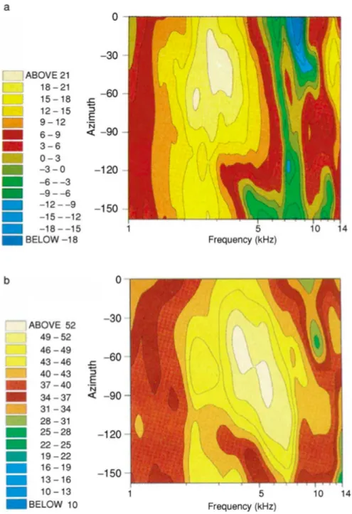
body of work for various elevations. All locations are along the midline, i.e. on the vertical plane that di-vides the left and right hemispheres. The azimuth and elevation of the recorded sound source for the differ-ent locations is labelled in degrees on the figure. . . 13 Figure 4 Variation in the spectral cues as a function of location
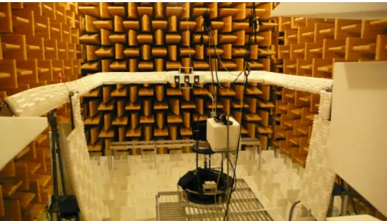
(changes in azimuth) of a sound source for the region of space directly ahead and left of the listener. Spec-tral variation is shown (a) for recordings from inside the ear canal using specialised microphones, and (b) at the level of detail that is likely to be encoded by the auditory system after passing through a cochlear filter. Frequency is plotted on a logarithmic scale and the gain of the filter is indicated by the color contours, which are arranged in 3 dB steps. Figure taken from (Carlile et al.,2005). . . 14 Figure 5 Example of the experimental setup for recordingHRTFs
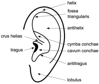
in an anechoic chamber. The listener is seated at the centre of the chamber with microphones in both ear canals while the mechanical arm with speakers at-tached moves up and down for different elevations. Different locations in azimuth are recorded by rotat-ing the chair the listener is seated on. . . 18 Figure 6 Labelled diagram of the human ear. Image taken from
Guillon(2009). . . 33
Figure 7 Diagram of the apparatus used to record the head-phone frequency responses. . . 53
xviii List of Figures
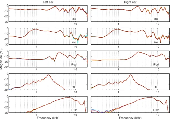
Figure 8 Headphone frequency responses for all the headphones used (except for the bone conduction) for the left and right ear. The magnitude responses for 10 replace-ments is shown using different colours on the plots. Only a small degree of variation is observed. . . 54 Figure 9 Exemplary recordings of a broadband gaussian noise
using the headphone equalisation (in red) for each of the headphones tested, except the bone conduction headphones. The recordings for the broadband stim-ulus using headphones without equalisation is shown in blue. . . 56 Figure 10 The headphone frequency response for the two bone
conduction headphones used in this study, provided by the manufacturer, shown in the top panels. The inverse of the frequency response (in red), along with the modelled inverse filter (in blue) is shown in the lower panels. . . 57 Figure 11 Scatter plots of lateral angle responses for all the
dif-ferent headphones tested. Response are presented on the vertical axes and target positions on the horizon-tal axis in degrees. The diagonal line corresponds to ideal responses. The size of the circles on the plots corresponds to the number of responses in a particu-lar 10◦by 10◦ grid. . . 63 Figure 12 Circular hair plots of polar angle errors for all the
headphone conditions tested. The subject responses have been collapsed across all lateral angles. The tar-get positions are represented by the small dots on the circles and the responses by the small segments orig-inating at these points. The direction of a response is determined by the direction that the small segment makes; the location of a response corresponds to the point at which the extended segment intersects the circle. An ideal response is thus a segment that is at a tangent to the small target dot on the circle, and a front-back confusion corresponds to a segment di-rected towards the opposite side of the circle. The value at the centre of each circular hair plot represents the circular correlation coefficient. . . 65
List of Figures xix
Figure 13 Results from Listening Test 1 in which judgements of either excellent, fair, or bad, corresponding to colours green, yellow, and red respectively, were made by each subject for the 46 HRTFsin the LISTEN database. The subject that made the judgement (subject number) is represented on the horizontal axis and theHRTFjudged (also indicated by subject number) is represented on the vertical axis. Subject number 10 did not make any judgements. . . 79 Figure 14 Virtual sound source trajectories in Listening Test 2.
The black line represents rendered positions. Red cir-cles represent the position directly in front of the lis-tener, at azimuth 0◦ and elevation 0◦, included in the figure as a reference. The larger blue circle at the cen-tre of the sphere represents the position of the lis-tener’s head. . . 82 Figure 15 A screenshot of the graphical user interface used for
Listening Test 1. . . 83 Figure 16 Subject responses for 51 differentHRTFsusing
Listen-ing Test 2. Each plot displays judgements from one subject for allHRTFsbetween end-point descriptors in-coherent (far left) and perfect (far right). . . 86 Figure 17 Standardised subject responses for 51 different HRTFs
using Listening Test 2. Each plot displays judgements from one subject for allHRTFsbetween end-point de-scriptors incoherent (far left) and perfect (far right). Re-sponses for each subject have been scaled and trans-lated to have a mean of zero and a standard deviation of one. . . 87 Figure 18 Three replicates of the author’s responses for the 51
differentHRTFsusing Listening Test 2.1. The standard-ised judgements are represented on the vertical axis increasing from bottom to top, corresponding to the end-point descriptors incoherent and perfect respectively. The judged HRTFs are represented on the horizontal
axis and are ordered in increasing positive judgement from left to right according to the third replicate. The responses for each HRTF are joined in order to repre-sent the degree of variation between trials. . . 90
xx List of Figures
Figure 19 Two replicates of the author’s responses for 26 dif-ferent HRTFs using Listening Test 2.2. The standard-ised judgements are represented on the vertical axis increasing from bottom to top, corresponding to the end-point descriptors incoherent and perfect respectively. The judged HRTFs are represented on the horizontal axis and are ordered in increasing positive judgement from left to right according to the second replicate. The responses for eachHRTFare joined by a line in or-der to represent the degree of variation between trials. 92 Figure 20 Three replicates of two subjects’ responses for five
dif-ferent HRTFs using Listening Test 2.3. The standard-ised judgements are represented on the vertical axis increasing from bottom to top, corresponding to the end-point descriptors incoherent and perfect respectively. The judged HRTFs are represented on the horizontal axis and are ordered in increasing positive judgement from left to right according to the third replicate. The responses for each HRTF are joined by a line in order to represent the degree of variation between trials. . . . 95 Figure 21 Graphical user interface used in the Listening Test 3. . 99 Figure 22 Three replicates of two subjects’ responses for five
dif-ferent HRTFsusing Listening Test 3 for attribute sense of direction. The standardised judgements are repre-sented on the vertical axis increasing from bottom to top, corresponding to the end-point descriptors inco-herent and perfect respectively. The judged HRTFs are represented on the horizontal axis and are arranged in ascending standardised judgement according to the third trial. The responses for each HRTFare joined by a line in order to represent the degree of variation be-tween trials. . . .100 Figure 23 Same figure as22for the attribute sense of distance
us-ing Listenus-ing Test 3. . . .100 Figure 24 Same figure as 22 for the attribute front image quality
using Listening Test 3. . . .101 Figure 25 Four replicates of two subjects’ responses for five
dif-ferentHRTFsusing Listening Test 3.1 for attribute sense of direction. The standardised judgements are repre-sented on the vertical axis increasing from bottom to top, corresponding to the end-point descriptors inco-herent and perfect respectively. The judged HRTFs are represented on the horizontal axis and are arranged in increasing standardised judgement according to the third trial. The responses for each HRTFare joined by a line in order to represent the degree of variation be-tween trials. . . .103
List of Figures xxi
Figure 26 Same figure as25for the attribute sense of distance us-ing Listenus-ing Test 3.1. . . .104 Figure 27 Same figure as 25 for the attribute front image quality
using Listening Test 3.1. . . .104 Figure 28 Same figure as25 for the attribute overall rating using
Listening Test 3.1. . . .105 Figure 29 Trajectories used for the two test stimuli. Black
cir-cles represent rendered positions. Red circir-cles repre-sent the position directly in front of the listener, at azimuth 0◦ and elevation 0◦, included in the figure as a reference. The larger blue circle at the centre of the sphere represents the position of the listener’s head. Trajectory 1 corresponds to the two attributes sense of direction and sense of distance, and Trajectory 2 corre-sponds to the trajectory front image quality. . . .109 Figure 30 Graphical user interface used in the Listening Test 3.2. 112 Figure 31 Box plots representing the spread of judgements for
HRTFsfor the attributes (a) sense of direction, (b) sense of distance, and (c) front image quality. Subjects are rep-resented on the horizontal axis and the HRTF judged is determined by colour and displayed on the legend. Judgements are represented on the vertical axis be-tween the labels Well and Not corresponding to the descriptor end-points well defined and not definable re-spectively. . . .115 Figure 32 Subject error variances across replicates, represented
on the horizontal axis, for each attribute judged as a function of assessor category (see table5), represented on the vertical axis. Attributes judged correspond to the colour of the circles and are labelled in the legend. Each circle is labelled with a number that corresponds to the subject that made the judgements. Circles vary slightly in terms of their vertical position within a par-ticular assessor category for ease of view. . . .118 Figure 33 (a) Number of auditions and (b) time taken for each
replicate performed. The time taken in minutes and the number of auditions is presented on the vertical axis and the replicate number on the horizontal axis. The different marker shapes correspond to the differ-ent subjects. . . .118
xxii List of Figures
Figure 34 Change in rank from one replicate to another for judged
HRTFs, for each subject, for the attributes (a) sense of direction, (b) sense of distance, and (c) front image qual-ity. The vertical axis is represented by the cumulative sum of change in rank across allHRTFsdivided by the total number of replicates. The horizontal axis corre-sponds to the number of replicates performed so that the value of two represents the change in rank from replicate one to two, and so on. . . .120 Figure 35 Mean error variance across subjects for the different
versions of the listening test. Note for Listening Test 3.2, only subjects categorised as either an expert or expert assessor were included. . . .121 Figure 36 Morphological parameters taken from the CIPIC database
of which 22 were used in this study. Figure taken from
Algazi et al. (2001b). . . .128
Figure 37 Visualisation of the input matrix for the Principal Com-ponent Analysis (PCA). . . .130 Figure 38 Mean inter-subject spectral difference across all
posi-tions, represented as black dots, as a function of fre-quency scale factor, for one pair subjects in the LIS-TEN database (subject 1025 and 1050). The red point displays the minimum mean frequency scale factor for this pair of subjects. Gray lines represent the calcu-lated inter-subject spectral difference for every posi-tion in space (i.e. each pair of measured subject Direcposi-tional Transfer Functions (DTFs)), from which the mean is calculated. . . .133 Figure 39 DTFsfor directions along the midline at elevations
rang-ing from in front to behind the listener (see text). The fractional octave-band filteredDTFsare presented for a pair of subjects without (unscaled) and with an optimal frequency scaling. For the scaled DTFs, sub-ject 1025 DTFs were scaled by a factor of 1.17 to the left and subject 1050 DTFswere scaled by 1.17 to the
right, for a combined optimal scale factor of 1.37. The vertical grid lines correspond to the frequency range used when calculating Inter-Subject Spectral Differ-ences (ISSDs). . . .134 Figure 40 CalculatedISSDvalues for one position (−45◦azimuth
and −45◦ elevation) as a function of Frequency Scale Factor (FSF) for when subject 1050 and 1025 are shifted first (blue and red respectively), along with the mean calculated for eachFSF(black). The bias for every sec-ond FSF is apparent for when either subject 1050 or 1025is shifted first. . . .136
List of Figures xxiii
Figure 41 Cumulative percentage of variance explained as a func-tion of Principal Component (PC) for aPCAof all con-catenated subjectDTFs. . . .140 Figure 42 Two metrics showing the reconstruction of each
sub-ject’s DTFs using PCs calculated from an input ma-trix of all subject DTFs except those of the subject in question. The left plot shows the cosine of the recon-structed and original concatenated subject DTFs, and the right plot shows the percentage mean squared error.142 Figure 43 Histograms of distributions, across all subjects, of
nor-malised distances between subjects andHRTFsjudged as either excellent (E), fair (F), or bad (B), for the six Multidimensional Spaces (MSs) using either: (a) fre-quency scale factors, (b) frefre-quency notches, (c) frac-tional octave-band filteredDTFs, (d) covert peaks, (e) un-filteredDTFs, or (f) morphology. The white + indicate distribution medians. All dimensions were used in eachMS. . . .144 Figure 44 Contour plots of F-ratio values for different frequency
ranges using all dimensions. F-ratio values are shown for MSs created via a PCA using two variants of the
HRTFdata: (a) non-filteredDTFs, and (b) fractional octave-band filteredDTFs. . . .146 Figure 45 F-ratio values for different frequency ranges for a
nar-row region of frequencies using an optimal selection of dimensions for (a) non-filtered and (b) filteredDTFs.
Each cell represents a frequency range. The shade of the cell corresponds to the effectiveness of theMSused; a darker shade translates to a more effectiveMS. . . . .147 Figure 46 Dimensions used for each frequency range for (a)
non-filtered and (b) fractional octave-band non-filteredDTFs re-spectively. The shade of the cells corresponds to the significance of the dimension; a black cell represents a dimension that was selected first for aMSand a white cell a dimension that was not selected. . . .150 Figure 47 The first three PCs for the position 0◦ azimuth and
0◦ elevation are shown in the upper plot. The red and green lines in bold represent the PCs that were the most effective, and the blue thin line represents a PC that was almost never selected. The lower plot of the figure displays subject DTFsfor the same posi-tion in space, colour-coded according to the sign of the weights of the first PC. . . .152
Figure 48 Histograms of distributions, across all subjects, of nor-malised distances between subjects andHRTFsjudged as either excellent (E), fair (F), or bad (B), for the six
MSs using either: (a) non-filtered DTFs, (b) fractional octave-band filteredDTFs, (c)FSFs, (d) frequency notches, (e) covert peaks, or (f) morphology. The white + indi-cate distribution medians. The optimal set of dimen-sions were used for each MS. . . .153 Figure 49 Histograms of distributions, across all subjects, of
dis-tances between subjects and HRTFs judged as either excellent, fair, or bad (labeled E, F, and B respectively) for the different MSsusing: (a) non-filtered DTFs and subjects’ calculated positions and (b) non-filteredDTFs
with a regression using morphological parameters. . .165 Figure 50 Example decision tree created for subject 1032 in the
database. Values on the branches show how instances are split based on a particular parameter at the node. The number of classified instances are shown in the rectangular boxes with the number of correctly/in-correctly classified instances indicated. . . .171 Figure 51 Percentage of correctly classified instances for each of
the subject-specific decision trees generated. Subjects for which no decision tree was generated are not dis-played. Decision trees that performed above chance (black line) are coloured green. . . .172 Figure 52 The number of times each of the eight optimal
mor-phological parameters appeared in the subject-specific decision trees across all subjects at each node level, along with the total count. The tally for each parame-ter is represented by the size of circles and their cor-responding colour. . . .173 Figure 53 Examples of the different pinna modifications on the
dummy head. Each modification is assigned a num-ber referring to the specificHRTFrecording and whether it was the left or right ear. . . .177
Figure 54 Each modification of the dummy head pinna displayed as a function of (a) the first and second, (b) the second and third PCweights from aPCA across all modifica-tions. . . .180
L I S T O F TA B L E S
Table 1 Table of the eight different headphones used in this study. Each headphone’s abbreviated name or ID, im-age, type, manufacturer, and model is displayed. Note that there is a headphone Tube Intra-aural (TI) op. that
is the exact same headphone as TI just that it sits at the entrance of the ear canal without blocking it. . . 46 Table 5 Summary of assessor categories employed in sensory
analysis, as defined in ISO/IEC IS 8586-2:1994 stan-dard, applied to the food industry and recommended for adoption in the field of audio. Table taken from (Zacharov and Lorho,2006). . . .107 Table 6 Error variance across replicates for each subject and
attributes sense of direction, sense of distance, and front image quality. . . .117 Table 8 Correlation coefficients comparing vectors of pairwise
distances between subjects in the six differentMSs. . . .155 Table 9 List of the different modifications for each recording.
The left and right ears were independently modified for a total of eight HRTF recording sessions, giving a total of 13 different modifications. . . .176
A C R O N Y M S
HRTF Head-Related Transfer Function
VAS Virtual Auditory Space
ITD Interaural Time Difference
ILD Interaural Level Difference
HRIR Head-Related Impulse Response
HpTF Headphone Transfer Function
xxvi a c r o n y m s
MUSHRA MUltiple Stimuli with Hidden Reference and Anchor
ISSD Inter-Subject Spectral Difference
PCA Principal Component Analysis
BEM Boundary Element Method
MaxIACC Maximum Inter-Aural Cross-Correlation
OC Open Circumaural
CC Closed Circumaural
TI Tube Intra-aural BC Bone Conduction
FR Frequency Response
SCC Spherical Correlation Coefficient
CCC Circular Correlation Coefficient
CC Correlation Coefficient
LSE LIMSI Spatialization Engine
GUI Graphical User Interface
ANOVA ANalysis Of VAriance
DTF Directional Transfer Function
MS Multidimensional Space
PC Principal Component
FSF Frequency Scale Factor
Part I
1
G E N E R A L I N T R O D U C T I O N
The current body of work aims at addressing the challenges to producing a compelling rendering of sound sources in Virtual Auditory Space (VAS) for the listener via the use of personalised Head-Related Transfer Func-tions (HRTFs). The work provides a potential solution to the laborious and
expensive task of recording individualisedHRTFsso that the technology be-comes more amenable to the consumer market. The research has been bro-ken up into four chapters:
1. Role of headphones in binaural synthesis (chapter 6) – assessment of the effect of the hardware used in producing binaural synthesis, namely the type of headphones used, and the effectiveness of a headphone equalisation, via a localisation task
2. Perceptual judgements ofHRTFsusing listening tests (chapter 7) – an itera-tive approach to developing a listening test that can be used to measure the effectiveness of binaural synthesis for different HRTFs, with an em-phasis on reducing the variability in subject responses and producing results with a high degree of repeatability
3. Salient spectral cues for binaural synthesis (chapter 8) – analysis of the most perceptually relevant spectral features in the HRTF using results from a listening test (from chapter 7) for a large number of subjects along with the subjects’ corresponding measuredHRTFs
4. Significant morphological parameters for binaural synthesis (chapter9) – val-idation of a method for predicting an optimal HRTF for a particular listener from a database, based on the results from chapter 8, using morphological parameters from the listener, along with an analysis of the significance of the different morphological parameters used Chapter6 explores an important component of binaural synthesis that is often overlooked; how the headphones used can determine the quality and realism of the rendering of sound sources in virtual auditory space. The fol-lowing three chapters7,8, and9, form part of a process that aims to be able to select an optimal HRTF from a database for a particular listener. Before developing this selection procedure, it was critical to have subjects be able to reliably evaluate the differentHRTFsin the database in order to determine whether a selectedHRTF was effective or not. To this end, the listening test developed in chapter7 established a method for minimising the variability in subject responses. The study in chapter8, whilst not using the optimal lis-tening test design from chapter7, involved an analysis establishing the most effective way to describe inter-subject differences based on measuredHRTFs. In the process of validating different methods for calculating inter-subject
4 g e n e r a l i n t r o d u c t i o n
differences, insights into which components of the HRTFwere the most per-ceptually salient were developed. These insights were considered relevant to the application of binaural synthesis to the consumer market given that they were grounded in perceptual judgements from a listening test assess-ing the quality of renderassess-ings inVAS. The most effective method for evaluating
HRTF inter-subject differences was then used in chapter 9 in order to create a model and a predictive procedure for selecting a personalised HRTF for a listener based on their morphology. Morphological dimensions of the outer ear and body were used from the same database from which the measured
HRTFs were taken. This type of predictive procedure has significant impli-cations for appliimpli-cations of binaural synthesis in the consumer market given that it bypasses the laborious and expensive task of recording individualised
HRTFswhilst ensuring a realistic rendering of sound sources inVAS.
With respect to the individual research chapters, beginning with chap-ter6, an analysis of the effect of headphone type on binaural synthesis was performed and considered important for potential applications of the tech-nology in the consumer market given that different headphones vary in their ability to produce a signal at all audible frequencies. The headphone types tested ranged from circumaural, to intra-aural, and even bone conduction headphones, which have different mechanisms for producing the signal at the listener’s ears. In addition, different headphones can add colouration to the signal that might be to the detriment of the quality of the rendering in
VAS. It is for this reason that a headphone equalisation was also tested. A localisation task was used for this study in order to be able to compare results with the large number of studies in the literature using virtual sound sources. This allowed for a quantitative assessment of the effectiveness of each headphone (with and without equalisation) to render a virtual sound source so that it was perceived at the target location in space.
The move from using a localisation task to using a listening test when as-sessing the quality of a binaural synthesis was made in chapter7in order to focus on aspects of a rendering that were particularly relevant to the applica-tion of the technology in the consumer market. Perceptual judgements for a number of different attributes of a rendering was considered more relevant localisation accuracy in this context. The iterative approach to designing the listening test used in the study was orientated towards questions relating to whether virtual auditory images appeared as being coherent or whether the rendering in general was realistic for the listener. A number of different listening test designs were used, each time aiming to eliminate biases that might cause variability in subject perceptual judgements across replicates of the listening test. One of the most significant changes made in this iterative process was a reduction in the number of different HRTFsbeing tested, and the use of specific attributes of the renderings rather a global judgement. The goal was to reach a point in the iterative process at which an acceptable de-gree of repeatability was observed among the subjects tested. Once this was achieved it would then be possible to use the responses for further analysis (i.e. for testing a method for selecting a personalisedHRTF).
g e n e r a l i n t r o d u c t i o n 5
The following phase of the research presented in this body of work in-volved both chapters8 and9. Both chapters relate to the design and valida-tion of a selecvalida-tion procedure that predicts an optimalHRTFfrom a database for the listener so that any rendering in VASwill be personalised. A range of solutions to the problem ofHRTF personalisation have been proposed in the literature, yet there is often a lack of a conclusive perceptual validation for the proposed techniques. This was one of the main motivations for the studies presented in these two chapters, in which a large number of subjects were tested in order to produce a statistically significant result.
Chapter 8 focuses mainly on using a number of different methods for describingHRTF inter-subject differences. Each method draws on a different aspect of theHRTFin terms of features in the spectrum that are important for a compelling rendering inVAS. The methods use either specific features, such as the notches that appear in the spectrum of theHRTF, or took into account all features in the spectrum. The inter-subject differences were used to pro-duce a multidimensional space in which all the subjects were represented; each subject corresponded to anHRTF from the database, and the closer the subjects were in the space to each other the more similar their HRTFs. Each of the methods, and corresponding multidimensional spaces, were validated using the perceptual judgements from a listening test.
An important factor in the analysis was the large number of subjects that participated in the listening test. Given that the study from chapter7showed that there is a high degree of variability in perceptual judgements for render-ings inVASusing differentHRTFs, it was important to have a large number of responses and an analysis that would be robust to ’noise’ in the results from the listening test (i.e. the assumed differences in perceptual judgements of the subjects if the listening test had been repeated).
The effectiveness of each of the multidimensional spaces in describing the perceptual judgements from the listening test was an indicator of the signifi-cance of theHRTFfeatures used in the analysis. This allowed for insights into the role and salience of some of the most commonly studied components of the HRTF. In addition to these insights, the statistical analysis enabled for
an understanding of the most perceptually relevant frequency ranges of the spectrum, based on a method of describing HRTF inter-subject differences that used all features in the spectrum.
The study in chapter 9 used the findings from the previous chapter. In particular, the most effective method for describing inter-subject differences and corresponding multidimensional space was selected and then used as the basis for a predictiveHRTF selection procedure. The approach took any subject’s morphology dimensions in order to position them into the mul-tidimensional space. Once a subject was placed in the space, the optimal
HRTFwas selected as the closest to that subject. The effectiveness of this pro-cess was tested by calculating the distances betweenHRTFsin the space for each subject in the database and comparing these distances to the percep-tual judgements from the listening test. In this way, the process could be refined by selecting different combinations of morphological parameters un-til the most effective subset was chosen. The predictive process of selecting
6 g e n e r a l i n t r o d u c t i o n
anHRTFfrom a database for a listener based on morphology was then shown to be statistically effective.
The mentioned subset of morphological parameters provided a further in-sight into what might be the most perceptually significant dimensions of a listener’s ear and body, in terms of their filtering effects in the HRTF. In essence, the analysis aimed to find the link between measured morpholog-ical parameters of a subject and HRTFs judged by the subject to be effective in VAS. This enabled a better understand how the body interacts with inci-dent waves from a sound source in space. The significance of the listener morphology was further developed by using only the listening test results and the subject morphological parameters (i.e. no HRTF data was included) and incorporating various machine learning algorithms. Decision trees were built using the perceptual judgements, and the morphological parameters were also ranked based on their relative importance as features in algorithm using support vector machines.
The final analysis of chapter 9 involved the use of HRTFs recorded on a mannequin head with replica pinnae made of rubber, cast from molds of real ears.HRTFrecordings were made for a number of modifications applied to the left and right ear replica pinna, such as completely filling a cavity with clay. The differences in the recordings across the different pinna modi-fications for a large number of locations in space showed how each morpho-logical parameter affected the HRTF. This in turn allowed for insights into the significance of the different modified parameters, given our knowledge of the role of the different spectral features in the HRTF from chapter8 and other studies. The different pinna modifications were also mapped into mul-tidimensional spaces in order to quantify their differences and understand how they compared to each other.
2
H U M A N A U D I T O R Y P E R C E P T I O N
This first chapter presents the fundamentals of how humans perceive their acoustic environment, and will act as a foundation to understanding the concepts of spatial audio detailed in this body of work. Our understanding of how the human auditory system works begins with an evolutionary per-spective. The ability of humans to encode mechanical disturbances in the medium in which they live, what we would call a sound, appears to have evolved to promote survival (Erulkar, 1972). It would be advantageous for a species, for example, to determine the location of predator’s approach or discern the call of a mate from a distance. To this end the auditory system would need to process sensory information in terms of the ’what’ and ’where’ of a sound; our current understanding is that of a dual-pathway model for encoding these two aspects with a binding of the two paths in the auditory cortex (see for exampleArnott et al.,2004).
Despite the fact that the visual system is a more developed and utilised sense in humans (in fact auditory perception has a heavy reliance on visual cues), the auditory system does a remarkably good job in terms of the per-ception of sounds in its own right. The human ear contains only a single receptive organ called the basilar membrane on which some 30,000 sensory cells, called hair cells, are responsible for registering the mix of all the differ-ent frequencies that make up our auditory environmdiffer-ent. This is an impres-sive feat due to the fact that at any one time there might be a combination of many sounds across different frequencies encoded on the basilar membrane and the auditory system is able to seamlessly interpret what we might call the different auditory objects around us (seeGriffiths and Warren,2004).
Humans have evolved to process a broad range of frequencies between 20Hz and 20 kHz. The level sensitivity of the human auditory system is so great that if it was any better we would hear the blood flow in our veins. We have highly specialised regions of the brain for detecting the ’what’ of sounds, such as for speech, and are capable of determining with much preci-sion the ’where’, or location, of sound sources without vipreci-sion. It is the ’where’ component of auditory processing that will be the focus of this body of work, and in particular how evolution has made use of the fact that we have two ears (Schnupp and Carr, 2009). The work endeavours to evaluate how the auditory system is able to perceive sounds in space and what aspects of the sounds might be important for effectively performing the task. Whilst explanations are mainly grounded in physiological and physical terms, it is important to note that the perception of the location of sound sources can be quite psychophysical as well (see for example the ventriloquist effect;Alais
and Burr,2004).
8 h u m a n au d i t o r y p e r c e p t i o n
2.1 c o o r d i nat e s y s t e m
In order to accurately describe the ’where’ of sound sources in space, a co-ordinate system must be implemented for the purposes of this research. In the current body of work, and in most studies, two coordinate systems will be used based on different poles. Figure1shows the two coordinate systems with the listener represented at the centre of an imaginary sphere. Figure1(a) shows what is what is known as the hoop coordinate system, in which the azimuth and elevation coordinates correspond to the standard single pole coordinate system where 0◦ azimuth and 0◦ elevation is directly ahead of the listener and positions to the right and up are positive (ranging from 0◦ to 180◦ and 0◦ to 90◦ respectively) and positions to the left and down are negative (ranging from 0◦ to −180◦ and 0◦ to −90◦ respectively).
Figure1(b) shows what is known as a lateral/polar coordinate system, in which there is a single pole passing through the two ears. The lateral angle is the horizontal angle away from the midline, which is the vertical plane separating the left and right hemispheres (i.e. the plane represented by the purple circle in figure2). Lateral angles to the left and right of the listener range from 0◦ to −90◦ and 0◦ to 90◦ respectively. For example, a lateral angle of 20◦ will describe all positions, at a fixed distance, on a vertical circle that subtend that angle from the median plane, whether it be in front or behind of the listener. The polar angle is the angle around the interaural axis (the axis connecting the left and right ear – represented by the green line in figure 2); this is the angle away from the horizontal plane on the described circle. Polar angles range from 0◦ to 180◦ from in front of the listener to behind in the upwards direction, and from 0◦ to −180◦ from in front to behind in the downwards direction. The lateral/polar coordinate system is a particularly intuitive one due to the fact that it mirrors how the auditory system determines sound source location (see section2.2.2).
2.2 au d i t o r y c u e s t o s o u n d l o c at i o n
The human auditory system has adapted to make use of the most salient acoustic cues from sound sources in our environment. Unlike other spatial senses such as vision where there is a topographic projection from receptor epiphelia into the central nervous system, the auditory system encodes the amplitude of the energy entering the ears as a function of frequency. Dif-ferences between the energy at the two ears is translated into information about the sound source’s location. As explained byBlauert(1997)
... the system does not use every detail of the complicated interau-ral dissimilarities, but rather derives what information is needed from definite, easily recognisable attributes.
It is also important to note that the auditory system uses a variety of different auditory cues depending on the environment (such as a reverberant room for example), which will be discussed below and detailed in chapter4.
2.2 auditory cues to sound location 9 0º to +180º 0º to -180º 0º to -180º 0º to +180º 0º to +90º 0º to -90º 0º to +90º 0º to -90º Hoop Lateral/polar Elevation Azimuth Lateral Polar
Figure 1: Representation of the two coordinate systems used in the current body of work: (a) hoop coordinate system, and (b) later/polar coordinate sys-tem. Red circles represent the position directly in front of the listener, at azimuth 0◦ and elevation 0◦, included in the figure as a reference. The larger blue circle at the centre of the sphere represents the position of the listener’s head.
10 h u m a n au d i t o r y p e r c e p t i o n
2.2.1 Dominant interaural cues
The Interaural Time Differences (ITDs) and Interaural Level Differences (ILDs) between the two ears for a single sound source in space are two crucial cues for determining location. ITDs refer to the difference in travel time of incident sound waves between the two ears for sound sources that are not on the midline (i.e. not at a point equidistant from both ears). For example if a sound were to originate to the right of a listener, the incident waves would arrive at the right ear before the left ear. Input from both ears meets at a structure along the auditory pathway known as the superior olivary complex that is sensitive to small time differences. The normal human threshold for detection of anITDis up to a difference of 10 µs with a relatively large degree of variance between individuals. Experiments conducted using a sphere to model the shape of the head, with a distance of approximately 22-23 cm between the two ears, measured maximum ITDs of approximately 660 µs (Woodworth and Schlosberg,1965).
Studies measuring the accuracy of listeners’ judgements of sound source location, or localisation tasks, using different stimuli suggest that whilst quency dependent interaural phase differences are detectable for low fre-quencies (Zwislocki and Feldman, 1956;Palmer and Russell, 1986) subjects are insensitive to them when an ITD is maintained (Kulkarni et al., 1999). Similar tests have shown that ITDs are probably encoded by mostly low-frequency auditory neurons (Middlebrooks and Green,1990) for frequencies below about 2 kHz (Blauert,1997).ITDsare also known to dominateILDcues for broadband stimuli (Wightman and Kistler,1992).
ILDs are caused by the absorption of energy primarily by the head and
also the body for sound sources off the midline, which produces a shadow-ing of the farthest ear. At low frequencies where the wavelength of sound approaches or is larger than the distance between the listener’s ears, the head does not diffract the incident waves and ILDsare quite weak and thus not a salient feature for localisation. Experiments with spherical head mod-els, using sounds with wavelengths much smaller than its diameter (i.e. the distance between the ears), have measured a maximum ILD of 6 dB for a sound source positioned along the interaural axis (Shaw, 1974). The mini-mum thresholds for ILDsare less than 1 dB (Mills, 1960). The auditory sys-tem most probably integrates level differences (and time differences) over discrete frequency channels, using the most salient and easily recognisable features available (Macpherson and Middlebrooks,2002).
2.2.2 Spectral cues
The interaural cues described previously are used by the auditory system to estimate a sound source’s position in space. HoweverITDsandILDsalone will not provide enough information for localisation in three-dimensional space; this is simply due to the fact that a specific interaural difference can describe any position in space that is equidistant to the listener’s ears. Equidistant points to a listener’s ears in space can be represented as a plane in the shape