Statistics for Topological Descriptors using optimal transport

HAL Id: tel-02979251

https://hal.archives-ouvertes.fr/tel-02979251v2

HAL is a multi-disciplinary open access

archive for the deposit and dissemination of sci-entific research documents, whether they are pub-lished or not. The documents may come from teaching and research institutions in France or abroad, or from public or private research centers.

L’archive ouverte pluridisciplinaire HAL, est destinée au dépôt et à la diffusion de documents scientifiques de niveau recherche, publiés ou non, émanant des établissements d’enseignement et de recherche français ou étrangers, des laboratoires publics ou privés.

transport

Theo Lacombe

To cite this version:

Theo Lacombe. Statistics for Topological Descriptors using optimal transport. Metric Geometry [math.MG]. Institut Polytechnique de Paris, 2020. English. �NNT : 2020IPPAX036�. �tel-02979251v2�

626

NNT

:

20

20

IPP

AX036

topologiques `a base de transport

optimal

Th`ese de doctorat de l’Institut Polytechnique de Paris pr´epar´ee `a l’ ´Ecole polytechnique ´Ecole doctorale n◦_{626 ´Ecole Doctorale de l’Institut Polytechnique de Paris (ED IP}

Paris)

Sp´ecialit´e de doctorat : Math´ematiques et Informatique

Th`ese pr´esent´ee et soutenue `a Palaiseau, le 8 septembre 2020, par

T

´

L

Composition du Jury :

Gabriel Peyr´e

Directeur de Recherche CNRS, ´Ecole Normale Sup´erieure (DMA) Pr´esident Peter Bubenik

Professeur, Universit´e de Floride (D´epartement de math´ematiques) Rapporteur Franc¸ois-Xavier Vialard

Professeur, Universit´e Gustave Eiffel (LIGM) Rapporteur Anthea Monod

Professeur assistant, Imperial College London (D´epartement de

math´ematiques) Examinateur Sayan Mukherjee

Professeur, Universit´e Duke (D´epartement de math´ematiques) Examinateur Steve Oudot

Charg´e de Recherche, Inria Saclay (Datashape) Directeur de th`ese Marco Cuturi

Je remercie tout d’abord les membres du jury qui ont chaleureusement accept´e de participer `a ma soutenance de th`ese, Sayan Mukherjee, Anthea Monod, Gabriel Peyr´e, et particuli`erement Peter Bubenik et Fran¸cois-Xavier Vialard qui ont rapport´e ce manuscrit qui conclut trois ann´ees de recherche. J’en profite pour signaler que cette th`ese a ´et´e rendue possible au moyen

d’un financement AMX de l’´Ecole polytechnique.

Je remercie mes directeurs de th`ese, Marco Cuturi et Steve Oudot, pour avoir guid´e mes premiers pas de jeune chercheur, pour la confiance et la libert´e qu’ils m’auront accord´ees en ayant toujours r´epondu pr´esents dans les moments importants. Merci aux autres membres permanents de l’´equipe DataShape, en particulier `a Fred pour l’aide que tu m’as apport´ee, `a Marc

pour toutes les fois o`u tu as bien voulu ´ecouter mes tergiversations

scien-tifiques. Aux post-docs que j’ai vu passer, Miro, Hari, Jisu, et ce sacr´e Martin. Merci aux doctorants qui m’ont montr´e la voie, Claire, J´er´emy, et

le respect´e docteur Mathieu qui m’a accueilli avec toute sa sympathie. `A

Nicolas pour m’avoir un jour parl´e de la TDA. Aux joyeux comp`eres qui sont arriv´es avec moi, Rapha¨el et Vincent. Aux plus jeunes qui viennent

mettre le chantier, Alex, Vadim, ´Etienne et Louis ; merci pour l’air frais

que vous avez amen´e. Une pens´ee pour le bon Younes avec qui j’ai bien ri. Aux camarades de l’ENSAE, Boris et Fran¸cois-Pierre, votre compagnie

quotidienne dans ce Slack d´esert ´etait plus que bienvenue. `A Christine,

St´ephanie et Bahar pour leur disponibilit´e et leur sympathie. Toutes ces personnalit´es ont rythm´e ma th`ese au quotidien et leur pr´esence se retrouve de pr`es ou de loin dans mon travail ; j’en profite pour remercier une seconde fois ceux avec qui j’ai eu la chance de collaborer : Steve et Marco, Mathieu, Fred et Martin, et enfin Vincent - travailler avec toi fut un plaisir.

Un grand merci `a tous ceux qui m’ont, `a un moment o`u un autre, fait me

sentir entour´e. `A mes amis de toujours, Jean-Baptiste, Arnaud et Vincent,

pour leur pr´esence inconditionnelle, mˆeme de l’autre cˆot´e du globe. Une pens´ee `a mes amis de pr´epa, L´ea, R´emy, Maxime, Paul, et bien d’autres,

avec qui je me suis form´e aux math´ematiques et `a la khontr´ee. Aux amis de l’X, Benoˆıt, R´emi, Victor, Pierre-Yves, Laure, le Bad’, le Forum et tous les autres. La petite ´equipe TSN, Raymond, Ilyes et Julien, toujours l`a

quand il fallait se changer les id´ees. `A tous les membres de ma famille, `a

Audrey et Charline pour tous ces moments pass´es ensemble, `a mes

grands-parents Jeannine, Jean et Josette qui m’ont inspir´e. `A mes fr`eres ador´es

Hugo et Dorian qui ont partag´e mon enfance et qui tracent maintenant leurs

chemins. `A mes parents qui ont cru en moi depuis le d´ebut ; cette th`ese,

c’est aussi le fruit de votre soutien.

Enfin, merci `a toi Lucie de continuer `a illuminer mes journ´ees `a l’aube de cette treizi`eme ann´ee qui, j’esp`ere, se terminera au pays du soleil levant.

1 Introduction 9

1.1 Introduction en fran¸cais . . . 9

1.2 Introduction in English . . . 20

2 Background 31 2.1 Topological Data Analysis . . . 31

2.2 Optimal Transport . . . 45

2.3 Notations . . . 59

I Theory

61

3.2 Persistence measures in the finite setting . . . 69

3.3 The bottleneck distance . . . 72

3.4 Duality . . . 76

3.5 Proofs . . . 79

4 Fr´echet means in the space of persistence measures 91 4.1 Fr´echet means in the finite case . . . 92

4.2 Existence and consistency . . . 93

4.3 Fr´echet means of persistence diagrams . . . 96

4.4 Proofs . . . 97

II Applications in statistics and learning

107

5 Fast estimation of Fr´echet means of persistence diagrams 109

5.1 Preliminary remarks and problem formulation . . . 110

5.2 A Lagrangian approach . . . 112

5.3 Entropic Regularization . . . 118

6 Linear representations 133

6.1 Continuity of linear representations . . . 133

6.2 Learning representations using PersLay . . . 137

7 Complementary examples 147

7.1 Expected persistence diagrams . . . 148

7.2 Quantization of persistence diagrams . . . 157

7.3 Shift-invariant distance . . . 167

Conclusion

178

Bibliography 183

Index 199

A Homology theory 203

A.1 Homology theory . . . 203

A.2 Filtrations and persistence modules . . . 207

A.3 Persistence diagrams . . . 212

B Elements of measure theory 221

1.1 M´elange de Gaussiennes . . . 10

1.2 Pr´eservation de la topologie par certaines transformations . . . 11

1.3 Topologie a diff´erentes ´echelles. . . 12

1.4 Diagrammes et distance de bottleneck . . . 14

1.5 Stabilit´e de la bottleneck . . . 15

1.6 Gaussian mixture . . . 21

1.7 Homotopy transformation . . . 22

1.8 Scale variant topology . . . 23

1.9 Diagrams and bottleneck distance . . . 25

1.10 Stability of the bottleneck distance . . . 26

2.1 Partial matching between two diagrams. . . 33

2.2 Stability of the bottleneck distance (sketch) . . . 35

2.3 Instability of cardinality of diagrams in sampling process . . . . 40

2.4 Cauchy sequence in the space of persistence diagrams . . . 41

2.5 Fr´echet mean of three persistence diagrams. . . 43

2.6 Optimal transport problem in 1D . . . 46

2.7 Transport map vs transport plan . . . 48

2.8 Wasserstein barycenter (example) . . . 51

2.9 Induced transport map in partial optimal transport . . . 54

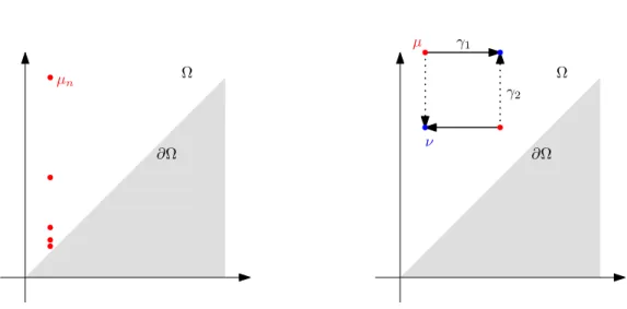
3.1 Illustration of differences between OTp, OT∞, and vague con-vergences. . . 75

4.1 Global picture of the proof of Proposition 4.4 . . . 99

4.2 Partition used in the proof of Lemma 4.7. . . 100

5.1 Example of output of Algorithm 1. . . 114

5.2 Local minimizers of the B-Munkres algorithm . . . 116

5.3 Error control in regularized OT . . . 121

5.4 Convolution in Sinkhorn algorithm (sketch) . . . 124 7

5.5 Parallelism in Sinkhorn algorithm (sketch) . . . 125

5.6 Regularized Barycenter estimation for persistence diagrams . . . 126

5.7 Fr´echet mean vs arithmetic mean . . . 128

5.8 Average running times for B-Munkres and Sinkhorn barycenters for persistence diagrams . . . 129

5.9 Qualitative comparison of B-Munkres and our Algorithm.. . . . 129

5.10 k-means in the space of persistence diagrams . . . 130

6.1 Some common linear representations of persistence diagrams . . 134

6.2 Orbits of dynamical systems . . . 141

6.3 PersLay (sketch) . . . 144

6.4 Learning the weight function. . . 145

7.1 Expected persistence diagram (example) . . . 149

7.2 Stability of expected persistence diagrams . . . 150

7.3 Quantization of persistence diagrams . . . 167

7.4 Cech diagram in log scaleˇ . . . 169

7.5 Persistence transform . . . 170

7.6 Non convexity of diagram distance up to translation. . . 171

7.7 Shift with a single point . . . 173

7.8 Shift-invariant distance . . . 179

A.1 An example of simplicial complex . . . 204

A.2 Singular simplex (sketch). . . 208

A.3 ˇCech and Rips complexes . . . 209

A.4 Algebraic pipeline to build persistence modules (sketch). . . 211

A.5 Filtration and persistence module (example) . . . 212

A.6 Persistence homology pipeline (example) . . . 217

Introduction

1.1

Introduction en fran¸

cais

1.1.1

Analyse des donn´

ees, statistiques et g´

eom´

etrie

L’analyse des donn´ees. L’analyse des donn´ees est devenue, au cours

de la derni`ere d´ecennie, un des domaines de recherche en math´ematiques appliqu´ees et en informatique les plus actifs et prolifiques. L’´evolution des moyens d’acquisition et des capacit´es de stockage en tout genre a permis de constistuer des collections de donn´ees colossales en tout genre : images

[KH+_{09], formes 3D [CFG}+_{15], sons [BMEWL11], donn´ees m´edicales et}

biologiques [CHF12], r´eseaux sociaux [YV15, KKM+_{16, PWZ}+_{17]... Le}

but de l’analyse des donn´ees est de comprendre et de valoriser ces nouvelles informations disponibles.

Pour cela, le paradigme le plus courant de nos jours est de recourir `a “l’apprentissage automatique”, dont l’id´ee g´en´erale est la suivante : pro-poser un algorithme capable d’extraire une information utile d’un jeu de donn´ees, permettant par exemple de r´ealiser de regrouper les donn´ees par similarit´e (clustering), d’attribuer des labels `a de nouvelles observations (classification), etc.

Statistiques et g´eom´etrie. Evidemment, il n’existe pas d’algorithme´

tout-puissant, qui serait capable de pr´edire sans erreur dans n’importe quel contexte. Si les observations et les labels ne sont pas ou peu li´es, ou si le nombre d’observations est trop faible, mˆeme le meilleur algorithme possible ne saura pas se montrer utile lorsqu’il s’agira d’extrapoler son apprentissage `a de nouvelles observations.

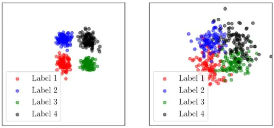
Figure 1.1: Nuages de 400 points tir´es selon un m´elange de quatre gaussiennes, repr´esentant quatre classes. Sur la figure de gauche, les gaussiennes ont une faible variance, et il est facile de s´eparer les diff´erentes classes. Sur la figure de droite, la s´eparation des classes est plus difficile.

La difficult´e `a r´esoudre un probl`eme d’apprentissage, par exemple sa d´ependance au nombre d’observations, peut se mesurer au moyen d’outils statistiques. Dans un probl`eme de classification ou de clustering par exem-ple, plus les observations d’une mˆeme classe (c-`a-d. partageant un mˆeme label) sont concentr´ees autour de leur moyenne (faible variance) et plus les classes sont distinctes, plus le probl`eme sera r´esolu efficacement (voir

Fig-ure1.1) De mani`ere g´en´erale, il est important de comprendre comment nos

observations sont distribu´ees. L’approche g´en´eralement adopt´ee en statis-tique est la suivante : nos observations sont ind´ependantes et proviennent d’une distribution de probabilit´e sous-jacente (inconnue). Connaˆıtre par-faitement cette distribution permettrait de comprendre le comportement des algorithmes d’apprentissage et d’optimiser leurs performances sur ce jeu de donn´ees (sans pour autant arriver n´ecessairement `a un score par-fait). En pratique, l’id´ee est donc d’estimer certaines propri´et´es de cette distribution sous-jacente `a partir de notre ´echantillon d’observations.

L’exemple le plus ´el´ementaire, et qui va nous amener `a des consid´erations g´eom´etriques, est l’estimation de l’esp´erance de la loi sous-jacente, c’est-`a-dire la valeur moyenne d’une observation tir´ee al´eatoirement. Ce probl`eme est en g´en´eral tr`es simple quand on observe des nombres r´eels : si on observe

(x1. . . xn) n nombres tir´es ind´ependamment selon une loi µ, un estimateur

de l’esp´erance de µ est simplement la moyenne arithm´etique des (xi)i,

c’est-`a-dire 1

n

Pn

Figure 1.2: `A gauche, un tore dont on identifie les propri´et´es topologiques. En-suite, un cercle, deux transformations qui en pr´eservent la topologie, et deux transformations qui ne les pr´eservent pas (d´echirement et recollement respective-ment).

la g´eom´etrie sous-jacente `a nos observations est g´en´eralement complexe et

inconnue : graphes, images, mol´ecules... autant de cas o`u la notion de

moyenne, et a fortiori des descripteurs statistiques plus sophistiqu´es, est difficile `a proprement d´efinir et estimer.

1.1.2

Descripteurs topologiques

Dans cette th`ese, nous nous int´eresserons `a un type d’observations en particulier, les diagrammes de persistance, qui proviennent de l’analyse

topologique des donn´ees. L’´etude de la g´eom´etrie sous-jacente `a ces

ob-jets, tout comme la conception et le calcul de descripteurs statistiques, sont des sujets de recherche actifs.

Topologie. Bri`evement, la notion de topologie renvoie `a celle de “forme”.

´

Etant donn´e un objet, par exemple une forme 3D, combien celui-ci poss`ede-t-il de composantes connexes ? Peut-on identifier des boucles caract´eristiques

`a sa surface ? Poss`ede-t-il des cavit´es ? Le tore repr´esent´e en Figure 1.2

poss`ede par exemple une composante connexe, deux boucles (en rouge), et une cavit´e (en bleu). Le cercle, lui, poss`ede une composante connexe et une boucle.

Dans un cadre plus g´en´eral, la topologie peut se comprendre comme les propri´et´es d’un objet qui sont pr´eserv´ees par des transformations continues,

sans d´echirement ni recollement, voir Figure 1.2. Par exemple, lorsqu’on

applique une telle transformation `a un cercle, si la g´eom´etrie de l’objet peut varier, sa topologie reste inchang´ee. D’un point de vue formel, les propri´et´es topologiques d’un objet sont d´ecrites par ses groupes d’homologie. Les groupes d’homologie d’un espace topologique (objet) sont d´ecrit par une

suite de groupe ab´elien (Hk)k(k = 0 correspond aux propri´et´es topologiques

de dimension 0, c’est-`a-dire les composantes connexes; k = 1 correspond aux boucles, k = 2 aux cavit´es, etc.) dont les g´en´erateurs indentifient les

t = 0 t = 1 t = 2 t = 3 t = 5 births deaths t t 0 1 2 2 3 5

Figure 1.3: Illustration du ph´enom`ene d’´evolution de la topologie `a diff´erentes ´echelles.

propri´et´es topologiques “ind´ependantes” de l’espace. Par exemple, pour

un tore, H1 a deux g´en´erateurs. Ceux-ci correspondent intuitivement aux

deux boucles rouges sur la Figure 1.2: toutes les autres boucles que l’on

peut dessiner sur le tore s’´ecrivent - en un sens - comme une combinaison

lin´eaire de ces deux boucles. Le lecteur int´eress´e peut consulter l’AnnexeA

ou [Mun84] pour une pr´esentation plus d´etaill´ee de la th´eorie de l’homologie.

Descripteurs multi-´echelles de la topologie. En pratique n´eanmoins,

l’usage de la topologie en apprentissage automatique n’est pas imm´ediat. La plupart des m´ethodes d’acquisition des donn´ees vont produire des objets sous forme de nuage de points, dont la topologie intrins`eque est

excessive-ment simple. Les groupes d’homologie d’un nuage de points (Hk)ksont

triv-iaux d`es que k≥ 1, tandis que H0 est le groupe ab´elien libre engendr´e par

N ´el´ements, o`u N d´esigne la cardinalit´e du nuage de points. L’homologie

seule n’est pas capable de refl´eter la structure sous-jacente de tels objets. L’id´ee fondamentale d´evelopp´ee dans les ann´ees 2000 (quoique les

fonde-ments peuvent ˆetre trac´es tout au long du XXe _{si`ecle) est de regarder}

la topologie d’un espace topologique `a diff´erentes ´echelles, et de regarder quelles sont les propri´et´es topologiques qui persistent `a travers celles-ci. Consid´erons par exemple le nuage de points repr´esent´e `a gauche sur la

Fig-ure 1.3. Initialement, il ne s’agit (topologiquement) que d’une collection

de composantes connexes ind´ependantes. Il apparait cependant naturel d’identifier trois boucles, de tailles diff´erentes. Regarder la topologie de cet objet `a diff´erentes ´echelles va nous permettre de d´etecter lesdites boucles. Pour introduire cette notion d’´echelle, une id´ee est de faire grossir des boules

centr´ees en chacun des points du nuage. Le param`etre d’´echelle t ≥ 0

cor-respond ici au rayon des boules. Ainsi, `a partir du nuage de points X

au param`etre t = 0, on construit une famille d’objets (Xt)t≥0. On parle

alors de filtration. Pour certaines valeurs critiques du param`etre t, voir

Figure1.3, la topologie1 _{change : des boucles apparaissent (par exemple `a}

t = 1 ou t = 2 sur la figure) ou disparaissent (lorsqu’elles sont compl`etement “remplies”, t = 2, t = 3, t = 5 sur la figure).

Ce sont ces valeurs critiques, appel´ees temps de naissance et de mort des propri´et´es topologiques, qui seront enregistr´ees dans un descripteur topologique : le diagramme de persistance. Un diagramme de persistance se pr´esente comme une collection de points dans le plan. La pr´esence d’un point de coordonn´ees (b, d) dans le diagramme va indiquer qu’une propri´et´e topologique (composante connexe, boucle, cavit´e...) est apparue `a l’´echelle t = b et a disparu `a l’´echelle t = d. Ainsi, un point proche de la diagonale,

c’est-`a-dire tel que d ' b, repr´esente une propri´et´e topologique qui est

ap-parue et a presque imm´ediatement disparu : cette propri´et´e a peu persist´e `a

travers les ´echelles. `A l’inverse, un point loin de la diagonale va repr´esenter

une composante topologique pr´esente durant un large intervalle d’´echelles, g´en´eralement consid´er´ee comme plus significative. Formellement, un

di-agramme de persistance est d´ecrit comme un multi-ensemble de points2

support´e sur le demi-plan

Ω :=_{{(b, d) ∈ R}2_{, d > b}

}

ou, de fa¸con ´equivalente, comme une mesure de Radon µ s’´ecrivant

µ :=X

x∈X

nxδx,

o`u X _{⊂ Ω est localement fini, n}x et un entier et δx d´esigne la masse de

Dirac en x∈ X.3

Bien entendu, le cadre d’application de l’analyse topologique des donn´ees ne se r´esume pas aux nuages de points et `a des boules qui grossissent ; la

th´eorie g´en´erale est pr´esent´ee dans la Section 2.1. `A ce stade, l’essentiel est

de retenir qu’il est donc possible de transformer une collection d’observations complexes en une collection de diagrammes de persistance, `a partir de laque-lle on peut envisager de produire une analyse statistique ou de r´ealiser une tˆache d’apprentissage automatique.

2_{Un ensemble dans lequel les points peuvent ˆetre r´ep´et´es}

3_{Dans leur d´efinition la plus g´en´erale, les diagrammes de persistance peuvent avoir}

des points avec des coordonn´ees infinies (b = −∞ or d = +∞) qui appartiennent donc au demi-plan ´etendu; ou des points sur la diagonale (b = d). Nous ignorons ces points dans cette th`ese, voir les Remarques2.2et 2.3.

yj0 proj(yj0) xi yj xi0 proj(xi0)

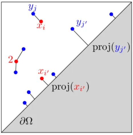
Figure 1.4: Deux diagrammes de persistance. La distance de bottleneck entre ces deux diagrammes est, par d´efinition, la longueur de la plus longue arˆete dessin´ee.

1.1.3

Diagramme de persistance et apprentissage:

limitations et enjeux

Les diagrammes de persistances portent une information riche et en g´en´eral compl´ementaire aux autres m´ethodes classiques d’analyse de donn´ees. Mal-heureusement, leur incorporation dans les outils modernes d’apprentissage, tels que les r´eseaux de neurones, n’est absolument pas ´evidente.

Distance entre diagrammes de persistance. Pour comprendre cela,

il faut dans un premier temps souligner qu’il est possible de mesurer une distance entre deux diagrammes de persistance, ce qui permet donc de com-parer les deux objets initiaux d’un point de vue topologique. La distance de r´ef´erence entre diagrammes est appel´ee distance de bottleneck, et se calcule

de la fa¸con suivante. Pour deux diagrammes X et Y , notons (x1. . . xn)

et (y1. . . ym) leurs points respectifs (notons qu’on n’a pas n´ecessairement

n = m). La premi`ere ´etape est de chercher `a transporter4 _{chaque point x}

i

du diagramme X vers un point yj de Y ou, ´eventuellement, vers sa

projec-tion orthogonale sur la diagonale (voir Figure 1.4). Les points yj de Y qui

ne sont pas atteints par un point xide X sont eux aussi transport´es sur leur

projection sur la diagonale. Nous imposons de plus que ce transport soit

bijectif : chaque point xi est envoy´e - au plus - sur un point yj, et chaque

yj doit ˆetre atteint par - au plus - un seul xi. En notant (xi, yj) quand xi

est transport´e sur yj, et (xi, ∂Ω) (resp. (∂Ω, yj)) lorsque xi (resp. yj) est

transport´e sur la diagonale, un transport partiel entre X et Y est d´ecrit par

une liste . . . (xi, yj)ij. . . (xi, ∂Ω) . . . (∂Ω, yj) . . . , o`u chaque point xi de X et

chaque point yj de Y apparaˆıt exactement une fois.

4_{On parle plus fr´equemment “d’appariement”, mais nous pr´ef`ererons la terminologie}

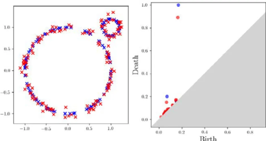
Figure 1.5: Illustration de la stabilit´e des diagrammes de persistance en bottle-neck, et instabilit´e du nombre de points.

Bien entendu, il existe une multitude de fa¸cons de transporter un dia-gramme X sur un autre diadia-gramme Y . Pour d´efinir la distance entre deux diagrammes, nous allons chercher un transport partiel optimal au sens

suiv-ant : le coˆut d’un transport partiel est la plus grande distance parcourue

entre deux points du transport. Un transport partiel optimal est un

trans-port partiel dont le coˆut est minimal parmi tous les transports partiels

entre X et Y possibles. Le coˆut minimal ainsi r´ealis´e est, par d´efinition,

la distance de bottleneck. Formellement, si on note Γ(X, Y ) l’ensemble des transports entre deux diagrammes X et Y , on pose

d∞(X, Y ) := min

γ∈Γ(X,Y )(x,y)∈γmax kx − yk.

Le choix de cette distance n’est pas arbitraire et est motiv´e par des

con-sid´erations alg´ebriques profondes qui sont d´etaill´ees dans la Section 2.1.

Cette distance jouit de la propri´et´e d’ˆetre stable, au sens o`u des objets

initialement proches auront syst´ematiquement des diagrammes proches en

distance de bottleneck (Figure 1.5).

Limitations. Etant donn´ee une collection de diagrammes, grˆace `a la dis-´

tance de bottleneck, il est possible de calculer des distances entre chaque paire de diagrammes. L’utilisation de certains algorithmes d’apprentissage basiques, comme celui du plus proche voisin, ou par exemple le

multi-dimensional scaling (MDS), est alors possible, car ceux-ci requi`erent

seule-ment de savoir calculer des distances entre nos observations (ici les dia-grammes).

N´eanmoins, la plupart des algorithmes modernes d’apprentissage de-mandent beaucoup plus de structure, qui va faire d´efaut dans le cadre des diagrammes de persistance. En effet, l’espace des diagrammes de persis-tance n’est pas lin´eaire, ce qui veut essentiellement dire qu’il n’est pas

pos-sible de donner un sens5 _{`a la somme de deux diagrammes de persistance,}

ou `a la multiplication d’un diagramme par un nombre r´eel. Il n’est donc pas possible d’incorporer na¨ıvement les diagrammes de persistance dans les machineries d’apprentissage modernes, et leur utilisation dans la pratique en est donc compromise.

Une solution de remplacement va consister `a plonger l’espace des dia-grammes dans un espace lin´eaire, sur lequel il sera donc possible d’effectuer des tˆaches d’apprentissage ais´ement. Cela signifie qu’on cherche une appli-cation Φ qui transforme les diagrammes en vecteurs, c’est-`a-dire un ´el´ement dans un espace lin´eaire. Une telle application est appel´ee une vectorisa-tion. Par exemple, une vectorisation naive pourrait consister `a associer `a chaque diagramme X son nombre de points Φ(X), plongeant l’espace des diagrammes dans l’espace des nombres r´eels, bien entendu lin´eaire. Cette vectorisation est tr`es d´ecevante car deux diagrammes tr`es diff´erents (au sens de la distance de bottleneck) peuvent avoir le mˆeme nombre de points, mais aussi deux diagrammes tr`es proches peuvent avoir un nombre de points tr`es

diff´erent (comme en Figure1.5). Autrement dit, Φ(X) n’a pas grand chose

`a voir avec X, ce qui est profond´ement regrettable.

Bien entendu, de nombreuses vectorisations bien plus satisfaisantes ont

´et´e propos´ees, avec d’importants succ`es dans les applications [Bub15,AEK+_17,

CCO17]. N´eanmoins, l’usage d’une vectorisation soul`eve quelques

interro-gations importantes :

• Le choix de la vectorisation est arbitraire. Parmi le large catalogue de vectorisations disponibles, il n’existe pas `a ce jour d’heuristique pour choisir laquelle sera adapt´ee `a une tˆache d’apprentissage donn´ee.

• Il semble impossible6 _{d’obtenir, en toute g´en´eralit´e, un plongement}

qui soit bi-stable, c’est `a dire pour lequel on aurait, pour toute paire

de diagramme X, Y , et deux constantes 0 < A_{≤ B < ∞,}

A_{kΦ(X) − Φ(Y )k ≤ d}∞(X, Y )≤ BkΦ(X) − Φ(Y )k,

ce qui aurait le m´erite d’assurer que des diagrammes proches ont des repr´esentations proches, et inversement.

5_{Qui serait compatible avec la distance de bottleneck}

6_{Ce probl`eme est encore ouvert, mais tous les r´esultats actuels semblent aller dans}

• Enfin, il faut rappeler que les diagrammes de persistance ont ´et´e con-struits en partie pour leur interpr´etabilit´e. Recourir `a une vectorisa-tion, et r´ealiser des calculs dans l’espace lin´eaire associ´e, retire cette interpr´etabilit´e. S’il est possible pour une collection de diagrammes

X1. . . Xnde calculer facilement une moyenne dans l’espace lin´eaire en

posant M = 1

n

Pn

i=1Φ(Xi), il est important de comprendre que cette

quantit´e n’a, a priori, rien `a voir avec une notion de moyenne dans l’espace des diagrammes de persistance. Cela vaut plus g´en´eralement pour toutes les op´erations r´ealis´ees dans l’espace lin´eaire (qui con-duiraient par exemple `a du clustering, etc.).

Enjeux. Si l’´etude des vectorisations de l’espace des diagrammes de

per-sistance reste un domaine de recherche pertinent, nous proposons ici de tra-vailler directement dans l’espace des diagrammes de persistance. L’objectif est donc de r´epondre `a la question

“Comment peut-on faire des statistiques dans l’espace des diagrammes de persistance ?”

Pour cela, il est important de comprendre d’abord quelles sont les pro-pri´et´es g´eom´etriques de cet espace, pour lequel nous ne disposons a priori que d’une distance pour en ´etudier la structure. Cela doit permettre en-suite de proposer un cadre th´eorique solide dans lequel des outils statistiques sont proprement d´efinis. Enfin, il est important que ces outils statistiques puissent ˆetre calcul´es et utilis´es, au moins de fa¸con approch´ee, en pratique.

1.1.4

Contributions et organisation du manuscrit

Afin de proposer des ´el´ements de r´eponse `a cette probl´ematique, nous nous appuierons sur un autre domaine des math´ematiques appliqu´ees : la th´eorie

du transport optimal, dont la pr´esentation est faite dans la Section 2.2. Il

s’agit peut-ˆetre du point essentiel de ce manuscrit : l’´etablissement d’un lien formel entre l’espace des diagrammes de persistance et les mod`eles

utilis´es en transport optimal. Cette connexion entre ces deux champs

math´ematiques est extrˆemement prolifique : le transport optimal est un domaine tr`es d´evelopp´e, tant dans sa th´eorie que dans les applications en statistiques et en apprentissage ; et nombre de ses outils s’adaptent `a l’´etude des diagrammes de persistance. Cela nous permettra d’obtenir de nouveaux r´esultats th´eoriques relatifs `a l’utilisation des diagrammes de persistance en statistiques et en apprentissage, mais aussi de proposer divers algorithmes et outils num´eriques qui permettent de r´esoudre des probl`emes difficiles

en persistance, comme l’estimation de moyennes (dites “de Fr´echet”), la quantification, l’apprentissage de vectorisation, entre autres.

De fa¸con g´en´erale, et sauf mention explicite du contraire, nous adoptons la convention suivante : les r´esultats (th´eor`emes, propositions, etc.) pour lesquels nous proposons une preuve sont le fruit de mon travail ou d’un travail joint avec mes collaborateurs : Mathieu Carri`ere, Fr´ed´eric Chazal, Marco Cuturi, Vincent Divol, Yuichi Ike, Steve Oudot, Martin Royer, et Yuhei Umeda.

Plan et lien avec les travaux r´ealis´es durant la th`ese.

Chapitre2: Pr´eliminaires. Ce chapitre pr´esente les deux domaines

im-pliqu´es dans ce travail: l’analyse topologique des donn´ees (Section 2.1) et

le transport optimal (Section 2.2). L’objectif est de pr´esenter rapidement

l’´etat de l’art relatif aux diff´erents probl`emes abord´es dans ce manuscrit. Notons n´eanmoins que la construction alg´ebrique des diagrammes de

per-sistance, developp´ee dans les sous-sections A.1etA.2, est ind´ependante du

reste du manuscrit.

Les contributions sont pr´esent´ees en deux parties, en fonction de leur nature th´eorique (propri´et´es g´eom´etriques g´en´erales, etc.) ou appliqu´ee (pour faire simple, conduisant `a une impl´ementation).

Partie I — Th´eorie.

Chapitre3: Un formalisme issu du transport optimal pour les

di-agrammes de persistance. Ce chapitre pr´esente et d´eveloppe les

fonde-ments th´eoriques de ce manuscrit. Son contenu repose essentiellement sur

la section 3 de l’article [DL19], en r´evisions mineures au Journal of Applied

and Computational Topology. Nous y pr´esentons comment les m´etriques utilis´ees habituellement pour comparer les diagrammes de persistance peu-vent se reformuler comme des probl`emes de transport optimal partiels, et les nombreux r´esultats th´eoriques qui en d´ecoulent.

Chapitre 4: Moyenne de Fr´echet pour les diagrammes de

per-sistance: aspects th´eoriques. Ce chapitre est consacr´e `a l’´etude des

moyennes de Fr´echet (ou barycentres) pour les diagrammes de persistance.

Il repose sur la section 4 de [DL19]. On y prouve notamment un r´esultat

d’existence tr`es g´en´eral, et on ´etablit un lien fort entre ces moyennes et les fameux “barycentres de Wasserstein”, largement ´etudi´es dans la litt´erature du transport optimal traditionnel.

Partie II — Applications.

Chapitre 5: Algorithmes efficaces pour l’estimation des moyennes

de Fr´echet des diagrammes de persistance. On propose ici un

al-gorithme pour approcher les moyennes entre diagrammes; particuli`erement efficace pour traiter les probl`emes `a grande ´echelle. Cette approche a ´et´e publi´ee dans les annales de la conf´erence internationale Neural Information

Processing Systems, 2018, voir [LCO18].

Chapitre 6: Repr´esentations lin´eaires des diagrammes de

persis-tance. Ce chapitre se consacre `a l’´etude des repr´esentations lin´eaires de

di-agramme de persistance, pour lesquelles on propose une caract´erisation

ex-haustive. Une fois encore, les r´esultats th´eoriques (Section6.1) sont issus de

[DL19, _{§5.1]. On propose ensuite une application de ce r´esultat en}

appren-tissage automatique en introduisant PersLay, une couche pour les r´eseaux

de neurones7 _{sp´ecifiquement ´elabor´ee pour apprendre des repr´esentations}

adapt´ees `a une tˆache donn´ee. Ce travail a ´et´e publi´e dans les annales de la

conf´erence Artificial Intelligence and Statistics, 2020, voir [CCI+_20].

Chapitre7: Exemples compl´ementaires. Ce dernier chapitre regroupe

diverses applications et algorithmes qui ont ´et´e d´evelopp´es afin de r´esoudre

divers probl`emes relatifs aux diagrammes de persistance. La Section 7.1

d´emontre l’int´erˆet du formalisme th´eorique d´evelopp´e dans le Chapitre 3

pour ´etudier les diagrammes de persistance dans un contexte al´eatoire. On y trouve des r´esultats de convergence et de stabilit´e pour des analogues

al´eatoires des diagrammes de persistance. La Section7.2´etudie la

quantisa-tion des diagrammes de persistance. Enfin, la Section7.3propose une fa¸con

simple et efficace pour estimer des distances entre diagrammes a

transfor-mation pr`es. Ces r´esultats n’ont pas encore ´et´e publi´es, mais les algorithmes

correspondant ont, ou vont ˆetre, int´egr´es `a la librairie d’analyse topologique

des donn´ees Gudhi[GUD15]; ce manuscrit de th`ese est une bonne occasion

d’en pr´esenter les rouages.

Code et contributions `a la librairie gudhi. La plupart des m´ethodes

pr´esent´ees en PartieIIont ´et´e, ou vont ˆetre, incorpor´ees `a la librairieGudhi.

1.2

Introduction in English

1.2.1

Data Analysis, Statistics, and Geometry

Data Analysis. Data analysis has become, during the last decade, one

of the most active research areas in applied mathematics and computer

science. Progress in data gathering and storage has led to very large

datasets of various types: images [KH+_{09], 3D shapes [CFG}+_15],

mu-sic [BMEWL11], medical and biological data [CHF12], social networks

[YV15, KKM+_{16, PWZ}+_{17]... Data analysis aims to understand and add}

value to such newly available information.

To do so, the most standard paradigm nowadays is to make use of “ma-chine learning”. It aims at designing algorithms that will be able to extract useful information from a given set of observations; allowing for instance to regroup data by similarity (clustering), to assign labels to new observations based on the labels of the training data (classification), etc.

Statistics and geometry. Of course, there is no omnipotent algorithm

that would be able to predict with no error in any context. If observations and labels are not correlated or if the number of observations is too low, even the best possible algorithm will not be of any use when it comes to generalizing its learning to new sets of observations.

The difficulty to solve a given learning problem, for instance its depen-dence on the number of observations, can be measured with statistical tools. In a classification or clustering problem for instance, the more the observa-tions sharing the same label are concentrated around their mean value (low variance) and the more the different classes are separated from each other,

the easier the problem will be to solve (see Figure 1.6). In general, it is

important to understand how our observations are distributed. The general approach taken in statistical learning is to assume that our observations are

independent and come from an (unknown) underlying probability

distribu-tion. Perfect knowledge of this distribution would allow us to understand the behavior of learning algorithms and to optimize their performances on a given dataset (without necessarily reaching a perfect score). In prac-tice, it is thus useful to infer some properties of the underlying probability distribution from our sample of observations.

The most basic example, which will lead to geometric considerations, is the estimation of the expectation of the underlying law, that is the average value of a randomly sampled observation. When the observations are real

numbers, this problem is pretty simple: if we observe (x1. . . xn) n numbers

Figure 1.6: Point clouds (400 points) sampled from a mixture of four Gaussian distributions, representing four classes. On the left subfigure, the Gaussians distributions have a low variance, it is thus easy to separate the different classes. On the right subfigure, class separation is harder to perform.

µ is simply given by the arithmetic mean of the (xi)is, that is _n1 Pn_i=1xi.

However, in modern machine learning problems, the underlying geometry of the observations is often complex and unknown: think of graphs, images, molecular structures... These are cases where the notion of mean, and

a fortiori more sophisticated descriptors, is hard to clearly define and to

estimate.

1.2.2

Topological Descriptors

In this thesis, we will focus on a specific type of observations: the persis-tence diagrams, which come from topological data analysis. Understanding the underlying geometry of these objects is an active research area, as is the design and the computation of statistical descriptors built on top of persistence diagrams.

Topology. Roughly speaking, the term “topology” is related to the notion

of “shape”. Considering a given object, such as a 3D shape, how many connected components does it have? Can we identify characteristic loops?

Does it have cavities? For instance, the torus represented in Figure1.7 has

one connected component, two loops (red), and a cavity (blue). In contrast, a circle has a single connected component and a single loop.

Figure 1.7: On the left, a torus and its topological properties. Then, a circle, two transformations that preserve its topology, and two transformations that do not (ripping and gluing respectively).

More generally, topology can be described as the set of properties of an object that do not change when we apply transformations without ripping

nor gluing (see Figure 1.7). For instance, when such a transformation is

applied to a circle, the topology (presence of one loop and one connected component) is unchanged, although the geometry is. Formally, the topo-logical properties of an object are described by homology groups. Homol-ogy groups of a topological space (object) consist of a sequence of abelian

groups (Hk)k≥0 (k = 0 accounts for 0-dimensional topological properties of

the space, that is connected components; k = 1 accounts for loops, k = 2 for cavities, and so on) whose generators identify “independent” topological

features of the space. For instance, in the context of a torus (Figure 1.7),

H1 has two generators. These would correspond intuitively to the two red

loops: any other loop on the torus is—in some sense—a linear combination

of these two loops. We refer the interested reader to AppendixAor [Mun84]

for a detailed presentation of homology theory.

Multi-scale topological descriptors. In practice however, the use of

topology in machine learning is not straightforward. Most data acquisition methods are likely to produce objects with an extremely simple topology,

such as point clouds. The homology groups of a point cloud (Hk)kare trivial

for k ≥ 1, while H0 is the free abelian group with N generators, N being

the cardinality of the point cloud. Homology alone is not able to reflect the underlying structure of such objects.

The core idea, whose foundations can be traced back to Morse’s work

[Mor40] and have been developed in [Fro92, Rob99, CFP01, ZC05], is to

consider the topology of a space at different scales, and to look for topolog-ical properties that persist through scales. Let us consider as an example

the point cloud represented on the left of Figure1.8. Initially, it is (from a

topological perspective) a collection of independent connected components. It is however intuitive to identify three loops of different sizes. Recording the topology of this object at different scales will allow us to detect these

t = 0 t = 1 t = 2 t = 3 t = 5 births deaths t t 0 1 2 2 3 5

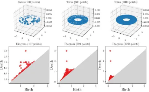
Figure 1.8: (Top) Topology of a point cloud at different scales for the ˇCech filtration. (Bot) The persistence diagram of the point cloud (restricted to loops).

loops. To introduce this notion of scale, an idea is to put balls centered on each point of the point cloud and to let them grow. The scale parameter

t ≥ 0 corresponds here to the radius of the balls. Therefore, starting with

a point cloud X at t = 0, we build an increasing sequence of topological

spaces (Xt)t≥0, called a ( ˇCech) filtration. For some critical values of t (see

Figure 1.8) the topology8 _{changes: loops appear (at t = 1, t = 1.5, t = 2 on}

the figure) or disappear (when they get “filled in”, at t = 2, t = 3, t = 5 on the figure).

These critical values, called birth times and death times, are recorded in a topological descriptor: the persistence diagram, which is a collection of points in the plane. Each point of coordinate (b, d) in the diagram will account for a topological property (connected component, loop, caveat...) that appeared at scale t = b and disappeared at scale t = d. Therefore, a

point close to the diagonal (that is, such that b _{' d) represents a topological}

property that appeared then almost instantly disappeared: this feature did not persist much. In contrast, a point away from the diagonal represents a topological feature that was recorded through a large interval of scales, gen-erally considered as being more significant. Formally, a persistence diagram

can be described as a multi-set of points9 _{supported on a half-plane}

Ω :={(b, d) ∈ R2

, d > b}

or, equivalently, as a point measure, that is a Radon measure µ of the form

µ = X

x∈X

nxδx,

where X is a locally finite subset of Ω, nx is an integer and δx denotes the

Dirac mass located at x_{∈ X.}10

Of course, the situations in which topological data analysis can be ap-plied are not reduced to point clouds and growing balls: the general theory

is detailed in AppendixA. The important point is that one can transform a

set of complex observations into a collection of persistence diagrams, from which we might consider producing a statistical analysis or performing a machine learning task.

1.2.3

Persistence diagrams and learning: challenges

and limitations

In practical applications, incorporating persistence diagrams in modern machine learning toolboxes, such as neural networks, is unfortunately not straightforward.

Distance between persistence diagrams. In order to understand this,

we must first mention that one can compute a distance between two per-sistence diagrams, which thus allows us to compare two objects adopting a topological viewpoint. The standard distance used to compare diagrams is called the bottleneck distance, and can be computed in the following way.

For two diagrams X and Y , let (x1. . . xn) and (y1. . . ym) denote their

re-spective points (note that we do not necessarily have n = m). The first step

is to transport11 _{each point x}

i in the diagram X to a point yj in Y or,

pos-sibly, to its orthogonal projection onto the diagonal (see Figure 1.9). The

points yj in Y which are not reached by a point xiin X are also transported

9_{A set where points can be repeated.}

10_{In the greatest generality, persistence diagrams can have points with infinite}

co-ordinates (b = _{−∞ or d = +∞) thus belonging to the extended half-plane; or points} supported exactly on the diagonal (b = d). We will not consider such points in this thesis; this is discussed in Remark2.2and Remark 2.3.

11_{It is more standard to use the wording “matching”, but we will prefer “transport”}

yj0 proj(yj0) xi yj xi0 proj(xi0)

Figure 1.9: Two persistence diagrams. The bottleneck distance between these two diagrams is given, by definition, by the length of the longest edge drawn here.

on their respective projections onto the diagonal. We also enforce that each

point xi is transported to—at most—a single point yj, and each yj must

be reached by—at most—a single xi. Denote by (xi, yj) the fact that xi is

transported on yj, and (xi, ∂Ω) (resp. (∂Ω, yj)) when xi (resp. yj) is

trans-ported to the diagonal. A partial transport between X and Y is given by

a list . . . (xi, yj)ij. . . (xi, ∂Ω) . . . (∂Ω, yj) . . . , where each xi, yj must appear

exactly once.

Of course, there exist many ways to transport a diagram X onto another diagram Y . In order to define a distance, one seeks for an optimal partial transport in the following sense: the cost of a partial transport is given by the longest distance traveled when performing the transport. A partial transport is optimal if it has minimum cost among all the possible partial transport between x and Y . The bottleneck distance is then defined as the minimal cost achieved by this optimal transport. Formally, let Γ(X, Y ) denote the set of all possible partial transports between X and Y , and define the bottleneck distance as

d∞(X, Y ) := min

γ∈Γ(X,Y )(x,y)∈γmax kx − yk.

The choice of such a distance is motivated by algebraic considerations

de-tailed in Appendix A and Section 2.1. This distance has the nice property

of being stable, in the sense that initially close objects will always have

dia-grams that are close in the bottleneck distance (Figure 1.10). For instance,

in the context of two point clouds P, P0 _{and corresponding diagrams µ, µ}0

built using the ˇCech filtration (Figure1.8), it yields

d∞(µ, µ0)≤ dH(P, P0),

where dH stands for the Hausdorff distance between the point clouds (see

Figure 1.10: Stability of persistence diagrams for the bottleneck distance. Here, the bottleneck distance between the two diagrams is controlled by the Hausdorff distance between the point clouds.

Limitations. Given a collection of diagrams, and thanks to the

bottle-neck distance, it becomes possible to compute pairwise distances between diagrams. It makes it possible to use these diagrams as the input of some simple machine learning algorithms, such as the nearest neighbor algorithm or the metric multi-dimensional scaling (MDS) one, as these algorithms only require to be able to compute distances between our observations (here, the persistence diagrams).

However, most modern machine learning algorithms ask for a linear structure on the space in which the data live. Unfortunately, the space of persistence diagrams is not linear, which essentially means that there is

no simple way12 _{to define the sum of two diagrams, or the multiplication}

of a diagram by a real number. Therefore, it is not possible to incorpo-rate faithfully persistence diagrams in a modern machine learning pipeline, compromising their use in practical applications.

An alternative is to embed the space of persistence diagrams in a lin-ear space, on which it will be possible to easily perform standard llin-earning tasks. It means that we look for a map Φ which transforms the diagrams into vectors, namely an element of a linear space. Such a map is called a vectorization.

Various vectorizations have been proposed, with significant success in

applications [Bub15,AEK+_{17, CCO17]. Nonetheless, using a vectorization}

raises some important questions:

• The choice of the vectorization is arbitrary. There is currently no heuristic available to choose, among all the possible vectorizations, which one will be adapted to perform well on a given learning task.

• It seems impossible13 _{to have, in the greatest generality, a coarse}

embedding, that is an embedding for which it holds, for any pair

of diagrams X, Y , and two non-decreasing map ρ1, ρ2 : [0, +∞) →

[0, +_{∞) with ρ}1(t)→ +∞ when t → +∞,

ρ1(d∞(X, Y )) ≤ kΦ(X) − Φ(Y )k ≤ ρ2(d∞(X, Y )),

which would ensure that close diagrams have close representations, and vice-versa.

• Finally, let us recall that diagrams benefit from their interpretability. Using a vectorization, and doing the computations in the correspond-ing linear space, would lose this interpretability. For instance, given

a map Φ and a set of diagrams X1. . . Xn, one can compute a mean

in the linear space by setting M = 1

n

Pn

i=1Φ(Xi). However, it is

im-portant to note that M has, a priori, nothing to do with a notion of mean in the space of persistence diagrams as it may not even be in the image of Φ. This holds more generally for any computation performed in the linear space (which could lead to clustering, etc.).

Challenges. While studying vectorizations of the space of persistence

di-agrams remains an important research topic, we propose in this manuscript to work in the space of persistence diagrams directly. The goal is thus to answer the following question:

“How can we do statistics in the space of persistence diagrams?” To answer this question, it is important to understand the geometric properties of this space. This should allow us to provide a solid theoretical framework in which statistical tools will be properly defined. Finally, these statistical tools must be usable in practice, that is we must be able to compute (or at least estimate) them.

13_{This problem is still open, but all recent results seem to point this way [BV18,}

1.2.4

Contributions and outline

To provide some solutions to this problem, we will rely on another field of

applied mathematics: optimal transport theory, presented in Section2.2. It

is one of the most important contributions of this manuscript: establish-ing a formal connection between the geometry of the space of persistence diagrams and models used in optimal transport. This connection between these two fields is highly useful: optimal transport is a well-developed do-main both from a theoretical and computational perspective and has many applications in statistical and machine learning. It turns out that most of its tools can be transposed or adapted to deal with persistence diagrams, which will allow us to obtain new theoretical results regarding the use of persistence diagrams in statistics and learning, but also to provide various algorithms and computational tools that allow us to address some difficult problems in topological data analysis, such as the estimation of Fr´echet means, quantization, vectorization learning, to name a few.

In general and unless stated differently, results (theorems, propositions, etc.) for which we provide a proof are consequences of my work or joint work with my Ph.D. advisors or collaborators: Mathieu Carri`ere, Fr´ed´eric Chazal, Marco Cuturi, Vincent Divol, Yuichi Ike, Steve Oudot, Martin Royer, and Yuhei Umeda.

Outline and relations with the research productions during the Ph.D. thesis.

Chapter 2: Background. This chapter presents the two fields involved

in this work: topological data analysis (Section2.1) and optimal transport

(Section2.2). It aims to provide a concise introduction to both domains and

a presentation of the different problems tackled in this manuscript. Note that a presentation of the algebraic construction of persistence diagrams

can be found in Appendix A.

The contributions are organized into two separate parts, according to their theoretical or applied (roughly speaking, results leading to an imple-mentation) nature.

Part I — Theory.

Chapter 3: an optimal transport framework for persistence

dia-grams. This chapter presents the theoretical foundations of the manuscript.

It essentially corresponds to Section 3 in [DL19], under minor revisions for

the standard metrics used to compare persistence diagrams can be reformu-lated as optimal partial transport problems, and the new theoretical results that come out of it.

Chapter 4: A theoretical study of Fr´echet means for persistence

diagrams. This chapter is dedicated to the study of Fr´echet means (or

barycenters) of persistence diagrams from a theoretical perspective. It

es-sentially corresponds to Section 4 in [DL19]. We prove the existence of

Fr´echet means in great generality, and establish a close link between those and the “Wasserstein barycenters”, their counterparts in standard optimal transport theory.

Part II — Applications.

Chapter 5: Fast algorithms for the estimation of Fr´echet means

of persistence diagrams. We propose an algorithm to estimate these

means, which is useful especially on large scale problems. This approach has been published in the proceedings of the international conference on

Neural Information Processing Systems, 2018 [LCO18].

Chapter 6: Linear representation of persistence diagrams. This

is dedicated to the study of linear vectorizations of the space of persistence diagrams, for which we provide an exhaustive characterization. The

the-oretical part (Section 6.1) comes from [DL19, §5.1]. We then provide an

application in machine learning, where we introduce PersLay, a neural

network layer14 _{devoted to learning optimal linear vectorizations to solve}

a given learning task. This work has been published in the proceedings of the international conference on Artificial Intelligence and Statistics, 2020

[CCI+_20].

Chapter 7: Complementary examples. This last chapter gathers

other algorithms developed for persistence diagrams. In Section 7.1, we

showcase the strength of the formalism developed in Chapter 3in the

con-text of random persistence diagrams. We prove convergence and stability

results of the probabilistic counterpart of persistence diagrams. Section7.2

is dedicated to the quantization of persistence diagrams, a useful tool that has benefits when incorporating persistence diagrams in machine learning

14_{including a publicly available implementation and incorporation to the Gudhi}

pipelines. Finally, Section 7.3 proposes a simple and efficient way to esti-mate a shift-invariant distance between persistence diagrams.

Code and contributions to the Gudhi library. Most of the methods

presented in PartII have been—or will be—incorporated into the

Background

Abstract

This chapter presents some background material coming from the two main research fields involved in this work: topological data analysis (Section2.1) and optimal transport (Section2.2). They are essentially presented in a way that serves the contents of PartI and Part II. Therefore, they do not aim at being exhaustive but rather at providing a decent state-of-the-art of the topics covered by this thesis.

2.1

Topological Data Analysis

This section is dedicated to the presentation of our objects of interest: per-sistence diagrams. A detailed algebraic construction of perper-sistence diagrams— which is not required to understand the vast majority of this manuscript—

can be found in Appendix A. We also refer the interested reader to [EH10,

Oud15] for a thorough description. Subsection 2.1.1 below gives a concise

presentation of these notions. Subsections 2.1.2 and 2.1.3 introduce

vari-ous metrics between persistence diagrams and some of the properties of the resulting metric spaces.

2.1.1

Persistent homology in a nutshell

Let X be a topological space, and f : X → R a real-valued continuous

function. The t-sublevel set of (X, f) is defined as

Ft={x ∈ X, f(x) ≤ t}.

Making t increase from−∞ to +∞ gives an increasing sequence of sublevel

sets (_Ft)t called the filtration induced by f . To the increasing family of

topological spaces (_Ft)t corresponds a persistence module (Vt)t, which is a

family of K-vector spaces (for some fixed field of coefficients K) equipped

with linear maps vt

s :Vs→ Vt for s≤ t which are induced by the inclusion

Fs ⊂ Ft (see Appendix A for details). In particular, for I = [b, d]⊂ R an

interval—withR = R∪{±∞}—, the interval module I[b,d]is the persistence

module defined byI_[b,d]t =K for t ∈ I, and {0} otherwise, while vt

s = idK if

s, t_{∈ I and v}t

s = 0 otherwise. Under mild assumptions (e.g. rk(vst) is finite

for any s, t), a persistence module (Vt)t can be decomposed uniquely as a

direct sum of interval modules, which reads

V =M

j∈J

I[bj,dj],

for some locally finite family of intervals ([bj, dj])j∈J. Therefore,V is entirely

described by a multiset1_{of points{(b, d)} that belong to the extended upper}

half-plane

R2≥ := {(b, d) ∈ R

2

, d_{≥ b},}

called the barcode, or persistence diagram, of (X, f), also denoted by Dgm(X, f)

or simply Dgm(f ) if there is no ambiguity.

Intuitively, an interval [b, d] appearing in Dgm(X, f) accounts for the

presence of a topological feature (connected component, loop, cavity, etc.)

that appears at scale t = b in (Ft)t and disappears (gets “filled”) at scale

t = d. Equivalently, a persistence diagram can be described as a point

measure supported onR2≥, that is a measure µ of the form

µ = X

x∈X

nxδx,

where X is a locally finite subset ofR2≥, nx is an integer, and δx denotes the

Dirac mass supported on _{{x}. This measure-theoretic perspective on}

per-sistence diagrams is motivated in [CDSGO16] (see also TheoremA.17) and

has huge benefits when studying the properties of the space of persistence

diagrams, as showcased in Chapter3.

2.1.2

Metrics between persistence diagrams

In order to use persistence diagrams in practice, we must—at the very least—be able to compare them using a metric. The standard metric used

1_{Points can be repeated in the family. The number of times a point appears in a the}

yj0 proj(yj0) xi yj xi0 proj(xi0) ∂Ω 2

Figure 2.1: Partial matching between two diagrams. The ‘2’ indicates that the point has multiplicity 2.

to compare persistence diagrams is the bottleneck distance, defined below. It is a partial matching distance between the points of the diagrams, counted

with multiplicity. We recall thatR2≥denotes the extended closed upper

half-plane. Let also ∂Ω denote the diagonal (this notation will be clarified later

on, in Definition 2.9):

∂Ω :=_{{(t, t), t ∈ R}.}

Definition 2.1. Let µ = Piδxi and ν =

P

jδyj be two persistence

di-agrams. Let X = (xi)i ⊂ R

2

≥ and Y = (yj)j ⊂ R

2

≥ be the points of the

diagrams, counted with multiplicity.

A partial matching γ is a subset of (X _{∪ ∂Ω) × (Y ∪ ∂Ω) such that}

any xi ∈ X (resp. yj in Y ) appears exactly once as a first (resp. second)

coordinate in γ (see Figure 2.1).

Let Γ(µ, ν) denote the set of partial matchings between µ and ν.

The cost of a matching γ _{∈ Γ(µ, ν) is defined as the length of the longest}

edge in the matching, that is max{kx − yk∞, (x, y)∈ γ}.

The bottleneck distance between the two diagrams is then defined as the

minimal cost that can be achieved by such a matching, that is

d∞(µ, ν) = inf

γ∈Γ(µ,ν)(x,y)∈γmax kx − yk∞. (2.1)

A partial matching that realizes this infimum is said to be optimal.

Remark 2.2. We start by noting some important remarks about these definitions.

• In the above definition, x (resp. y) belongs either to X or to the

diag-onal ∂Ω. If x _{∈ X has finite coordinates and is matched to ∂Ω, that}

is it belongs to a tuple (x, y) _{∈ γ with y ∈ ∂Ω, then one can always}

assume that y is the orthogonal projection of x onto the diagonal as

this would only reduce the cost.

• Similarly, although a partial matching might theoretically contain

cou-ples (x, y) ∈ ∂Ω × ∂Ω, these can be removed when looking for an

optimal matching as this does not increase the cost.

• Persistence diagrams might contain points that belong to ∂Ω, in which case they can always be matched to the diagonal (with themselves) with a null cost. In particular, the bottleneck distance is only a

pseudo-metric at this stage. This aspect will be clarified in the following

subsection.

• In the standard definition of the bottleneck distance, k · k∞ stands for

the L∞ _{norm in R}2_{, although it can be replaced with any norm k · k}

q

with1≤ q ≤ ∞. Adapting the following results is straightforward due

to the equivalence of norms in R2. Whenq does not play any role, we

simply use the notation _{k · k.}

Remark 2.3. Persistence diagrams may contain points with coordinates

of the formx = (b, +_{∞) (resp. (−∞, d)). The set of such points is called the}

essential part of the diagram. When comparing two persistence diagrams, if the cardinalities of their essential parts differ, the cost of any matching

(thus the bottleneck distance) is +_∞.

Otherwise, the points of the respective essential parts must be matched together for the cost to be finite, and it is straightforward to observe that optimally matching those points consists in sorting the points with respect to their first (resp. second) coordinate and then using the increasing match-ing. It mostly means that the behavior of essential parts is obvious and independent of the rest of the diagrams.

In the rest of this manuscript, we will therefore only consider persistence diagrams with empty essential parts. Most of our theoretical and practical results can be easily adapted to take the essential parts into account sepa-rately.

Using the bottleneck distance to compare persistence diagrams is

mo-tivated by algebraic considerations detailed in Appendix A. In addition,

Figure 2.2: Stability of the bottleneck distance for the ˇCech diagrams with respect to the Hausdorff distance between the point clouds.

[CSEH07, CCSG+_{09a], which states that two close filtrations induce close}

persistence diagrams in the bottleneck distance.

Theorem 2.4 (Stability theorem). Let f, g : X → R be two q-tame

func-tions (they induce q-tame persistence modules, see Appendix A), and let

Dgm(f ), Dgm(g) be their respective persistence diagrams. Then,

d∞(Dgm(f ), Dgm(g))≤ kf − gk∞, (2.2)

that is the operator f _{7→ Dgm(f) is 1-Lipschitz, that is:}

Example A.21in Appendix A provides a simple application in the

con-text of diagrams built on top of point clouds. Briefly, if P and P0 _{are two}

finite point clouds in Rd_{, one has}

d∞(Dgm(dP), Dgm(dP0))≤ d_H(P, P0),

where dP (resp. dP0) denotes the distance to P (resp. P0), and d_H(P, P0) is

the Haussdorf distance between P and P0_{: similar point clouds have similar}

persistence diagrams. This fact is illustrated in Figure 2.2.

Other metrics of interest. From a theoretical perspective, the

bottle-neck distance is a natural choice to compare persistence diagrams. However, when used for statistical and machine learning applications, it has some im-portant drawbacks. Indeed, given two diagrams µ and ν and an optimal

partial matching γ∗_{, the bottleneck distance between µ and ν only depends}

on the longest edge in γ∗_{. It means that}

• Any matching, as long as it does not change the length of the longest

edge in γ∗_{, will also be optimal. There are therefore plenty of optimal}

matchings between two diagrams in general.

• Similarly, a slight perturbation in the points in µ, as long as it does not change the length of the longest edge of an optimal matching, will not be detected in the bottleneck distance.

In statistical and machine learning applications, discriminating information might lie in these undetected properties. Therefore, in practice, a variation of the bottleneck distance is usually preferred.

Definition 2.5. Let 1 ≤ p < ∞. The p-th distance between two

dia-grams µ and ν is defined as

dp(µ, ν) =   inf γ∈Γ(µ,ν) X (x,y)∈γ kx − ykp q   1 p . (2.3)

In (2.3), k · kq stands for any q-norm, with 1≤ q ≤ ∞. Natural choices

are q = 2 (Euclidean ground metric), q = p, and q = _{∞. This choice has}

barely any impact on the theoretical results presented in the manuscript.

The choice q = p might have benefits in numerical problems (see Chapter5)

as it leads to a separable cost.

While dp → d∞ as p → ∞, it improves on the drawbacks mentioned

above: the optimal partial matching between two diagrams (for the dp

metric) is generically unique, its cost involves all the edges of the matching (making this distance able to account for small perturbations), etc. The p-th diagram distance also satisfies a (weaker) stability property.

Definition 2.6. A metric space X is said to imply a bounded

degree-q total persistence if there exists a constant C_X such that for every tame

Lipschitz function f : X → R, with Lip(f) ≤ 1, one has Persq(Dgm(f ))≤

C_X, where Persq(Dgm(f )) := dq(Dgm(f ), 0) =   X x∈Dgm(f ) kx − ∂Ωkq   1 q , (2.4)

Theorem 2.7 ([CSEHM10]). Let X be a triangulable, compact metric

space that implies bounded degree-q total persistence for some q _{≥ 1, and}

f, g : X → R two tame Lipschitz functions. There exists a constant C_X that

depends on X such that for all p ≥ q,

dp(Dgm(f ), Dgm(g))≤ CX(max Lip(f )q, Lip(g)q)

1

pkf − gk1−

q p

∞ . (2.5)

Remark 2.8. The p-th distances between persistence diagrams are gen-erally referred to as “Wasserstein distances” between persistence diagrams,

a terminology that comes from optimal transport theory, see Section 2.2

below. As optimal transport will take a big place in this manuscript, we use the word “Wasserstein” to denote standard optimal transport metrics to avoid confusion.

2.1.3

Statistics and machine learning with

persistence diagrams

Let us end this section by introducing important notions for the develop-ment of this manuscript. Namely, we start by defining and stating the main properties of the space of persistence diagrams. We then present some statistical and machine learning problems that take place in this space.

Recall (Remark 2.3) that we only consider diagrams whose points have

finite coordinates.

The space of persistence diagrams

We can now compare persistence diagrams using either the bottleneck or

the p-th distances (for the sake of simplicity, we use the notation dp for

both metrics). It invites us to consider the space of all possible diagrams equipped with such metrics.

First, note that the wording “metrics” is actually improper as the bot-tleneck and the p-th distances are only pseudo-metrics in the sense that one

can have dp(µ, ν) = 0 while µ 6= ν. This is due to the points in the

dia-grams that lie on the diagonal ∂Ω, as those can be matched to the diagonal with a cost of 0. This leads to a natural equivalence between diagrams: two persistence diagrams are equivalent if their off-diagonal parts coincide. The resulting equivalence classes will still be referred to as persistence dia-grams. From a practical perspective, this is equivalent to simply removing the points lying on the diagonal. We can now give our core definitions.

Definition 2.9. Let us define the open upper half-plane

Ω :=_{{(b, d) ∈ R}2_{, b < d}

}, (2.6)

and note that the diagonal ∂Ω :={(t, t), t ∈ R} is its boundary.

A persistence diagram is a point measure supported on Ω, that is a

measure of the form

µ = X

x∈X

nxδx,

where X is a locally finite subset of Ω, and nx ∈ N.

The set of all persistence diagrams will be denoted by _D.

Essentially, this definition is consistent with the algebraic one developed in the previous subsection, where diagrams are understood without their essential parts (as it is treated separately in a trivial manner) and points on

the diagonal are removed (as those cannot be detected by the dp distances).

These assumptions allow recovering true metric spaces on which we can provide a relevant analysis.

Definition 2.10. Let µ ∈ D, and 1 ≤ p ≤ ∞. The total persistence of µ of parameter p is

Persp(µ) := dp(µ, 0)∈ [0, +∞], (2.7)

where 0 denotes the empty diagram.

The space of persistence diagrams of parameter p is

Dp

:= {µ ∈ D, Persp(µ) <∞}. (2.8)

This definition was introduced in the seminal papers [MMH11,TMMH14].

The assumption Persp(µ) < ∞ in (2.8) ensures that for any µ, ν ∈ Dp, the

quantity dp(µ, ν) is finite. It makes (Dp, dp) a metric space. Note the

convenient expression, for 1_{≤ p < ∞,}

Persp(µ) =

X

x∈X

nxkx − ∂Ωkp = µ(k · −∂Ωkp), (2.9)

where _{kx − ∂Ωk denotes the distance between a point x ∈ Ω and (its}

orthogonal projection onto) the diagonal ∂Ω. When p = _{∞, note that}

Pers∞(µ) = supx∈Xkx − ∂Ωk.

The space of persistence diagrams, at least for finite p, satisfies some fundamental properties.