Ultrasound contrast imaging with multi-pulse transmission

(1)

HAL Id: tel-01018646

https://tel.archives-ouvertes.fr/tel-01018646

Submitted on 4 Jul 2014

HAL is a multi-disciplinary open access archive for the deposit and dissemination of sci-entific research documents, whether they are pub-lished or not. The documents may come from

L’archive ouverte pluridisciplinaire HAL, est destinée au dépôt et à la diffusion de documents scientifiques de niveau recherche, publiés ou non, émanant des établissements d’enseignement et de

Fanglue Lin

To cite this version:

Fanglue Lin. Ultrasound contrast imaging with multi-pulse transmission. Signal and Image processing. INSA de Lyon, 2013. English. �NNT : 2013ISAL0117�. �tel-01018646�

(2)

THESE

Ultrasound Contrast Imaging with

Multi-pulse Transmission

Délivrée par

L’INSTITUT NATIONAL DES SCIENCES APPLIQUEES DE LYON

Pour obtenir

DIPLÔME DE DOCTORAT

École doctorale:

ELECTRONIQUE, ELECTROTECHNIQUE, AUTOMATIQUE

Soutenue publiquement le 14 Novembre par

Fanglue LIN

Jury

Co-directeur de thèse :

Olivier BASSET Professeur des Universités, Université Claude Bernard, Lyon I Professeur des Universités, Université Claude Bernard, Lyon I Christian CACHARD

Rapporteur :

Philippe MARMOTTANT Charge de Recherche CNRS, HDR, Université Joseph Fourier, Grenoble I Directeur de Recherche INSERM, Tours

Ayache BOUAKAZ Examinateur :

François TRANQUART Directeur de Recherche, Bracco Suisse Professeur des Universités, INSA de Lyon

Professeur des Universités - Praticien Hospitalier, Université d'Auvergne Denis FRIBOULET

(3)

CHIMIE

http://www.edchimie-lyon.fr

Insa : R. GOURDON

M. Jean Marc LANCELIN Université de Lyon – Collège Doctoral Bât ESCPE 43 bd du 11 novembre 1918 69622 VILLEURBANNE Cedex Tél : 04.72.43 13 95 directeur@edchimie-lyon.fr E.E.A. ELECTRONIQUE, ELECTROTECHNIQUE, AUTOMATIQUE http://edeea.ec-lyon.fr Secrétariat : M.C. HAVGOUDOUKIAN eea@ec-lyon.fr M. Gérard SCORLETTI Ecole Centrale de Lyon 36 avenue Guy de Collongue 69134 ECULLY Tél : 04.72.18 65 55 Fax : 04 78 43 37 17 Gerard.scorletti@ec-lyon.fr E2M2 EVOLUTION, ECOSYSTEME, MICROBIOLOGIE, MODELISATION http://e2m2.universite-lyon.fr Insa : H. CHARLES

Mme Gudrun BORNETTE CNRS UMR 5023 LEHNA

Université Claude Bernard Lyon 1 Bât Forel 43 bd du 11 novembre 1918 69622 VILLEURBANNE Cédex Tél : 06.07.53.89.13 e2m2@ univ-lyon1.fr EDISS INTERDISCIPLINAIRE SCIENCES-SANTE http://www.ediss-lyon.fr Sec : Samia VUILLERMOZ Insa : M. LAGARDE

M. Didier REVEL Hôpital Louis Pradel Bâtiment Central 28 Avenue Doyen Lépine 69677 BRON Tél : 04.72.68.49.09 Fax :04 72 68 49 16 Didier.revel@creatis.uni-lyon1.fr INFOMATHS INFORMATIQUE ET MATHEMATIQUES http://infomaths.univ-lyon1.fr

Sec :Renée EL MELHEM

Mme Sylvie CALABRETTO Université Claude Bernard Lyon 1 INFOMATHS Bâtiment Braconnier 43 bd du 11 novembre 1918 69622 VILLEURBANNE Cedex Tél : 04.72. 44.82.94 Fax 04 72 43 16 87 infomaths@univ-lyon1.fr Matériaux MATERIAUX DE LYON http://ed34.universite-lyon.fr Secrétariat : M. LABOUNE PM : 71.70 –Fax : 87.12 Bat. Saint Exupéry

Ed.materiaux@insa-lyon.fr

M. Jean-Yves BUFFIERE INSA de Lyon

MATEIS

Bâtiment Saint Exupéry 7 avenue Jean Capelle 69621 VILLEURBANNE Cedex

Tél : 04.72.43 83 18 Fax 04 72 43 85 28

Jean-yves.buffiere@insa-lyon.fr

MEGA

MECANIQUE, ENERGETIQUE, GENIE CIVIL, ACOUSTIQUE

http://mega.ec-lyon.fr Secrétariat : M. LABOUNE PM : 71.70 –Fax : 87.12 Bat. Saint Exupéry

mega@insa-lyon.fr

M. Philippe BOISSE INSA de Lyon

Laboratoire LAMCOS Bâtiment Jacquard 25 bis avenue Jean Capelle 69621 VILLEURBANNE Cedex Tél :04.72 .43.71.70 Fax : 04 72 43 72 37 Philippe.boisse@insa-lyon.fr ScSo ScSo* http://recherche.univ-lyon2.fr/scso/ Sec : Viviane POLSINELLI

Brigitte DUBOIS Insa : J.Y. TOUSSAINT

M. OBADIA Lionel Université Lyon 2 86 rue Pasteur 69365 LYON Cedex 07 Tél : 04.78.77.23.86 Fax : 04.37.28.04.48 Lionel.Obadia@univ-lyon2.fr

(4)

ABSTRACT

In ultrasound imaging domain, nonlinear imaging, which utilizes the nonlinear backscattered signals, has become an important branch. Nonlinear imaging, also named harmonic imaging, can be divided into tissue harmonic imaging and contrast harmonic imaging, according to where the nonlinear signals come from. Contrast harmonic imaging emerges because contrast agents, which are intravenously injected to enhance the weak echoes backscattered from blood cells, can vibrate nonlinearly when they undergo a acoustic pressure higher than a threshold. Then, these nonlinear signals backscattered by contrast agents are collected to form harmonic images where the linear echoes backscattered from surrounding tissue are supposed to be removed. However, during the wave propagation in tissue, the interaction between the acoustic wave and tissue medium modifies the wave shape and the harmonics of the transmitted wave are also generated in tissue. The presence of tissue harmonic signals, merged with harmonic signals from contrast agents, degrades the image quality in contrast harmonic imaging.

This thesis aims to better distinguish the echoes from contrast agents and the echoes from tissue, whether through designing new modalities, or investigating and optimizing the existing modalities. Our efforts are mainly focused on the multi-pulse techniques in ultrasound contrast imaging.

Firstly, we propose a mathematical background to generalize most of the multi-pulse ultrasound imaging techniques that have been described in previous literatures. The formulation can be used to predict the nonlinear components in each frequency band and to design new transmission sequences to either increase or decrease specified nonlinear components in each harmonic band. Simulation results on several multi-pulse techniques are in agreement with the results given in previous literatures.

Secondly, the techniques using multiple transmissions to increase the CTR are generally based on the response of static scatterers inside the imaged region. However, scatterer motion, for example in blood vessels, has an inevitable influence on the relevance of the techniques. It can either upgrade or degrade the technique involved. Simulations, vitro experiments from a single bubble and clouds of bubbles, and

in-vivo experiments from rats show that the phase shift of the echoes backscattered from

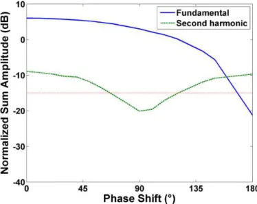
bubbles is dependent on the transmissions’ phase shift, and that the bubble motion influences the efficiency of multi-pulse techniques. Fundamental and second-harmonic amplitudes of the summed signal change periodically, exhibiting maximum or minimum values, according to scatterer motion. Furthermore, experimental results based on the second-harmonic inversion (SHI) technique reveal that bubble motion

(5)

can be taken into account to regulate the pulse repetition frequency (PRF). With the optimal PRF, the CTR of SHI images can be improved compared to second-harmonic images.

Besides of these considerations relative to generalization and scatterer movement in multi pulse techniques, a new technique, called double pulse inversion (DPI), has also been proposed. The PI technique is applied twice before and after the arrival of the contrast agents to the region of interest. The resulting PI signals are substracted to suppress the tissue-generated harmonics and to improve CTR. Simulations and

in-vitro experimental results have shown an improved CTR of DPI. However, the

presence of tissue movements may hamper the effectiveness of this technique. In-vivo experimental results confirm that the tissue motion of the rat during the acquisition is an inevitable barrier of this technique.

(6)

ACKNOWLEDGMENT

Firstly, I would like to thank Prof. Philippe Marmottant and Prof. Ayache Bouakaz for their acceptance to be the reviewer of this thesis and their effort to review this thesis manuscript. I am also grateful to the other members of the jury, Prof. François Tranquart, Prof. Denis Friboulet and Prof. Armand Abergel, for their willingness to discuss the work during the defense.

Three years ago, when I finished my Master study in Southeast University in Nanjing, I had a strong willingness to go outside to see the “western world”. Therefore, I am very happy to be given the opportunity to pursue my Ph.D. degree in Lab CREATIS in France. I would like to thank my supervisors, Prof. Olivier Basset and Prof. Christian Cachard, for choosing me from the list of applicants. I would also thank Prof. YueMing Zhu, who is responsible for this application program and Prof. Isabelle Magnin, who is the director of the lab, for their approval to my application. I would also show my gratitude to China Scholarship Council (CSC) for the financement during my Ph.D. study.

Special thanks should be given to my supervisors, Prof. Olivier Basset and Prof. Christian Cachard. Your broad scientific view and your enthusiasm to research always inspire me. Your patience and kindness help me pass through the difficult time at the very beginning when I cannot say a single French word. Also thank you for the guidance, the weekly discussions and the corrections to all my papers.

I would like to also acknowledge Prof. Piero Tortoli, Dr. Francesco Guidi, Dr. Riccardo Mori and Dr. Alessandro Ramalli for their warm reception, selfless sharing of their experience and useful help during our collaboration. Also thank you for the real Italian pizza and Italian espresso coffee. I am also grateful to Dr. Aymeric Guibal, who spared his time to help us with the clinical tests.

Ultrasound group in our lab is not only a professional group, but also a friendly group. I am lucky to have these colleagues and make friends with them. François, you are a good example of a researcher. Your smartness, creativity and hardworking impresses me. Thank you for your numerous help and I learned a lot from you. Matthieu, with your warm smile, it is a pleasure having scientific or non scientific conversations with you. Thank you for every detailed explanation to French phrases and French culture. Thank you for being my “tourist guide” during our short stay in Florence. Adeline, with your presence in the ultrasound room, experiments become more efficient when something is missing, not working or needed. Thank you for your assistance. Hervé and Denis, you are very easy-going. Life seems more colorful with your big smile and laughter. Bakary, you are a nice officemate with a good temper. It

(7)

was a pleasure sharing an office with you. Sébastien, still remember the short stay in Dresden as my neighbor? Thank you for sending me back in the dark.

During the past three years, I have also made friends with some Chinese students: Feng, Lihui, Yue, Xinxin, Yan, Hongjiang, Changyu, Hongying, Shengfu and Liang. I have many unforgettable memories with you: the “tea time”, the dinner parties, the travel… I also find it interesting to discover the difference between our southern and northern culture in everyday life. I cherish our friendship.

At last, I like to appreciate the support and unconditional love from my parents. Their optimism and open-minded attitude towards the life always give me courage every time when I feel depressed. Pei, the distance between Lyon and Grenoble does not separate us, it makes us closer. Thank you for always being there, for sharing my happiness and sadness, for wiping my tears and fears, for everything.

(8)

Chapter 1

1. Introduction

Every day, we touch with sound, a very common and intuitive physical phenomenon. Then what is sound? Sound is a mechanical wave in nature: a wave that is created by oscillating objects and that propagates through a medium (gas, liquid or solid). An important parameter to describe sound, or acoustic wave, is frequency �. According to frequency, sound can be classified to infrasound, audible sound and ultrasound. The frequency of the audible sound, which is perceptible by human ears, is from about 20 �� to 20 ��. Then the acoustic wave having a frequency higher than 20 �� is called ultrasound while that having a frequency lower than 20 �� is called infrasound. As a mechanical wave, sound propagation depends on the properties of the medium. So the physical quantities related to medium, such as pressure �, density � and sound velocity � , are also important. The effects like reflection, refraction, scattering, attenuation, absorption are usually involved in the various applications of sound.

Ultrasound, because of its good directivity, high spatial resolution or high energy, has been applied in various domains, such as underwater detection, industrial flaw detection, distance measurement, mechanical pieces cleaning and alloy production. Besides of these, ultrasound has also been widely used in medical diagnosis, thanks to its safety, real-time property and low cost compared to other medical assisted devices, and in medical treatment like in HIFU (High Intensity Focused Ultrasound) techniques.

For medical ultrasound, the propagation medium is the organs in human body. In biological tissue, the average sound velocity is around 1540 �/�. The frequency of the diagnostic ultrasound is usually in the range between 1.5 �� and 15 ��. So the wavelength of medical ultrasound wave is between 1 �� and 0.1 ��. Because the wavelength is larger than the medium particle, or the obstacle, scattering is the dominant effect happening when the ultrasound wave travels through the biological medium. The backscattered signals from all the medium particles during the wave travelling path are captured by the transducer and displayed as an ultrasound image, which can show the anatomy structure of the insonified region.

1.2 Thesis objective

Conventionally, the backscattered signals are collected to form an ultrasound image. Nowadays, nonlinear imaging, which utilizes the nonlinear backscattered signals, has become an important branch in ultrasound imaging domain, mainly because nonlinear imaging provides an improved resolution. Nonlinear imaging, also named harmonic imaging, can be divided into tissue harmonic imaging and contrast harmonic imaging, according to where the nonlinear signals come from.

(14)

Contrast harmonic imaging emerges because contrast agents, which is intravenously injected to enhance the weak echoes backscattered from blood cells, can vibrate nonlinearly when they undergo a high acoustic pressure, then these nonlinear signals backscattered by contrast agents are collected to form harmonic images, to distinguish the linear echoes backscattered from surrounding tissue. Contrast harmonic imaging is commonly used to help the diagnosis of the cardiovascular disease through observing the anatomical structure of blood vessel, and abdominal organ cancer through observing tissue perfusion dynamics.

However, as already mentioned above, nonlinear signals can also come from tissue. During the wave propagation in tissue, the interaction between the acoustic wave and tissue medium modifies the wave shape, so the harmonics of the transmitted wave are generated. The presence of tissue harmonic signals is merged with the harmonic signals from contrast agents and degrades the image quality in contrast harmonic imaging.

Therefore, the thesis objective is to better distinguish the echoes from contrast agents and the echoes from tissue, whether through designing new modalities, or investigating and optimizing the existing modalities.

1.3 Layout of the thesis

In this thesis, efforts are mainly focused on the multi-pulse techniques in ultrasound contrast imaging. The manuscript is divided into the following four parts:

• Introduction part: Chapter 1 leads the readers into the topic of this thesis by a general introduction of medical ultrasound, thesis objective and layout of the thesis.

• Background part: This part introduces the necessary background knowledge in ultrasound nonlinear imaging. Chapter 2 describes the linear and nonlinear behaviors of contrast agent bubbles and presents different models generally used. Chapter 3 presents the nonlinear phenomenon of wave propagation, the equations used to describe the nonlinear propagation, and then introduces two simulators used in this thesis.

• Contribution part: This part presents my original works on the nonlinear imaging, especially on the multi-pulse techniques in ultrasound contrast imaging. Chapter 4 generalizes most of the multi-pulse techniques applied in contrast imaging, using a single formula. This formula can be used to predict each nonlinear component in each harmonic band. Simulations have been conducted to validate this formula. Chapter 5 investigates the influence of bubble movement to multi-pulse techniques. Simulations and experimental results on a single bubble and a cloud of bubbles are presented. Based on these results, the optimization of second harmonic inversion (SHI) imaging, a

(15)

recently proposed multi-pulse technique, is also presented. Chapter 6 proposes a new modality named double pulse inversion (DPI), using the pulse inversion technique twice, to reduce the tissue-generated harmonics to increase contrast-to-tissue ratio (CTR). Simulations and experimental results are presented. • Conclusion and perspectives part: Chapter 7 concludes the contributions of this

(16)

(17)

Chapter 2

2. Ultrasound contrast agents

Contrast agents are expected to be persistent enough to complete the diagnosis process, small enough to move into capillaries and pass through pulmonary circulation, and inert enough not to alter hemodynamics. Nowadays, contrast agents are usually gas-filled and encapsulated. The acoustic properties of contrast agents are strongly influenced by the kinds of capsule material. So efforts have also been taken to the measurement of acoustic properties of microbubbles and to the production of them.

This chapter introduces the linear and nonlinear behavior of a free gas microbubble in section 2.2, and then presents the characteristics, the models and the medical applications of ultrasound contrast agents in section 2.3. At last, a short conclusion is given in section 2.4.

2.2 Microbubble

The diameter of a microbubble is on the order of micron. As it is much smaller than ultrasound wavelength (between 0.1 �� to 1 �� ), the bubble behaves like a Rayleigh scatterer.

2.2.1 Linear behavior

Air bubble in water has a cross section 100 million times greater than that of the iron sphere having the same radius, because of the significantly different compressibility of the gas bubble [De Jong (1993)].

An air bubble has a flexible boundary with surrounding fluid. The response of the bubble depends on two factors: the springlike stiffness of the gas and the inertia of the fluid. The balance between the two factors can leads to the resonant frequency:

�� = 1 2��₀�

3�_��₀

� (2.1)

where �₀ is the equilibrium bubble radius, �_� is the ratio of heat capacities at constant pressure and constant volume, �₀ is the static pressure at the bubble surface and � is the density of the surrounding liquid.

When there is an acoustic pressure on the bubble, the bubble contracts and expands with this external force.

(19)

When the pressure amplitude is large, a bubble can expand more than compress. Recently it has also been found that some bubbles had “compress-only” behavior [De Jong et al. (2007)]. These asymmetric vibrations lead to nonlinear response of bubbles. Lord Rayleigh [Rayleigh (1917)] was the first one to describe the behavior of a microbubble by an equation, this equation has been improved by Plesset [Plesset (1949)], Nolting and Nepiras [Noltingk et al. (1950)], and Poritsky [Poritsky (1952)]. All these contributions lead to the Rayleigh-Plesset equation:

��̈ +3�̇₂2 = 1 � ��0 + 2� �0 − �� 0 � � 3κ +�_�− �₀−2� � − 4��̇ � − �� (2.2)

where �₀ is the equilibrium bubble radius, � is the liquid density, �₀ is the static pressure at the bubble surface, �_� is the liquid vapor pressure, � is the damping term for the shear viscosity of the fluid, � is the surface tension term, κ is the polytropic gas index. � is the time-varying radius of the bubble, acted on by a time-varying acoustic pressure �. �̇ and �̈ are the velocity and the acceleration of the bubble surface. Equation (2.2) describes the dynamics of a free gas bubble without shell in an incompressible fluid.

2.3 Ultrasound contrast agents

2.3.1 Characteristics of ultrasound contrast agents

Different from air bubbles, a contrast agent usually has a shell outside the gas core. The majority of these gases are perfluorocarbon-like gases or air, and the shells vary from serum albumin to surfactants. The diameter of contrast agents is about 1-10 �� and the thickness of the shell is about 10-200 ��.

With the presence of the shell, the expansion of a contrast agent is constrained and the resonant frequency is raised. So the resonant frequency becomes:

��2 =��2 +₄_��₂�_� (2.3)

where �_� is the stiffness of the shell, � is the effective mass of the system, and �_� is the free gas bubble resonance expressed by equation (2.1).

Before talking about the behavior of these contrast agents, the concept of mechanical index (MI) should be introduced. MI is a parameter to estimate the likelihood of inertial cavitation with an intervening tissue path:

�� = ��′ ��

(2.4) where �_� is the center frequency (�� ), �_�′ is the maximum axial value of rarefactional pressure measured in water (��), �_�(�), multiplied by an in situ exponential factor:

(20)

��′= ��[��(�)�−0.0345��] (2.5) In United States, the allowed maximum MI for medical ultrasound imaging is 1.9 [Szabo (2004)].

The behavior of contrast agents under acoustic excitation depends on the exciting pressure and frequency, and the structure of the microbubbles:

�� ℎ��ℎ ��

(2.6)

2.3.2 Models of ultrasound contrast agents

To well understand the behavior of contrast agents, efforts have been done to model the vibration of the contrast agent microbubbles.

2.3.2.1 Rayleigh-Plesset model

The basic equation to describe oscillating gas bubble is the Rayleigh-Plesset equation, which has been presented in equation (2.2) and is rewritten here:

��̈ +3�̇₂2 = 1 � ��0 + 2� �0 − �� 0 � � 3κ +�_�− �₀−2� � − 4��̇ � − �� (2.7)

This equation is applicable to a spherically symmetrical free gas bubble in an incompressible fluid, but the effect of shell is missing [Leighton (1994)].

2.3.2.2 De Jong model

The model proposed by De Jong et al. modifies the basic Rayleigh-Plesst equation to take into account shell and other damping effects as well as shell forces. The shell is assumed to be extremely thin. With the presence of the shell, the stiffness of the contrast agent is strengthened and the sound damping is increased. Therefore, instead of the viscosity damping of the fluid, a total damping parameter is given [De Jong et

al. (1992)]:

�� =��+��+��ℎ+�� (2.8)

where �_�� is the viscous damping, �_�� is radiation damping, �_�ℎ is thermal conduction damping and �_� is damping due to friction within the shell. So together with a shell elastic parameter �_� used to describe the shell-restoring force, the modified equation is given [De Jong et al. (1993)]:

��̈ +3�̇2 2 = 1 � ��0� �0 � � 3κ +�_�− �₀−2� � − �� 1 �0− 1 �� − ��0��̇ − �� (2.9)

where �_�0 is the initial pressure inside the bubble and �₀ is the center pulsation of the excitation wave. The parameters �_� and �_� were determined by experimental measurements on Albunex bubbles.

(21)

2.3.2.3 Hoff model

The model proposed by Hoff et al. accounts for the finite thickness of the shell and forces, elastic nature of the shell in a more accurate way. A more accurate description of the effects of the shell have been presented by Hoff et al. [Hoff et al. (2000)] based on Church model [Church (1995)]. The shell thickness is modeled as a viscoelastic layer that changes thickness in proportion to the stretching of the dynamic radius.

��̈ +3�̇2 2 = 1 ��0�� 0 � � 3κ − 1� − 4��̇_{� −}12��0�0 2 �3 �̇ � − 12��0�0 2 �3 �1 − �0 � � − �� (2.10)

where �_� and �_� are the densities and the shear viscosity of the surrounding liquid, ��0, �� and �� are the initial thickness, the shear viscosity and the shear modulus of the shell. In this equation, two shell parameters, the shear modulus �_� and the shear viscosity �_�, were determined from measurements on experimental bubbles from Nycomed.

2.3.2.4 Marmottant model

Another model can describe the behavior that microbubble can break up when the driving pressure is high enough [Marmottant et al. (2005)]. A surface tension varying with bubble radius is added. The equation is:

��̈ +3�̇₂2 = 1 � ��0+ 2� �0 − �� 0 � � 3κ �1 −3_{� �}κ ̇� − �0− 2�_� � −4_{� ��}�̇ �−κ_{� � − ��}� (2.11)

where the surface tension is defined as:

�� = ⎩ ⎪ ⎨ ⎪ ⎧ 0 � ≤ �� λ �_� �2 �� 2 − 1� �� ≤ � ≤ �� ≥ �� (2.12)

The rupture radius �_{��}, the bucking radius �_{��} were determined by experimental measurements on SonoVue and BR14 bubbles, which have phospholipid shells.

There also exist many other models. More details can be found in the review paper by Allen et al. [Allen et al. (2002)] and Faez et al [Faez et al. (2013)].

2.3.3 Applications of ultrasound contrast agents

The application of ultrasound contrast agents falls into two scopes: diagnosis and therapy.

(22)

One major diagnostic application is opacification, which is the brightening of a blood pool. For example, the blood pool volume of the left ventricle of the heart is tracked to determine the ejection fraction to measure the function of the heart acting as a pump, or to identify irregular local wall motions of the endocardium under stress testing [Szabo (2004)]. Another diagnostic application is perfusion, which is the amount of blood delivered into a local volume of tissue per unit of time. For example, perfusion of myocardium can be measured, and regions where blood cannot reach may indicate ischemia or infarct; perfusion of other tissues can indicate angiogenesis or increased vascularization in tumors and the location of lesions [Szabo (2004)].

For therapeutic applications, contrast agents are designed to carry drugs to targeted sites and release medication by ultrasound-induced fragments, in order to avoid wasting large amount of medications throughout the body, to prevent unwanted side effects, and to ensure the drugs are delivered to the intended sites. For example, the agents can find and bind with thrombi and vulnerable plaque [Lindner (2001)]. The agents can also deliver cytotoxic drugs to angiogenesis sites to prevent feeding tumor growth [Lindner (2001)].

2.4 Conclusion

In this chapter, a brief review about ultrasound contrast agents is presented. This thesis mainly pays attention to the nonlinear responses or the harmonics of these contrast agents because the thesis objective is to detect and distinguish the harmonic signals generated by contrast agents and by tissues.

(23)

Chapter 3

3. Nonlinear ultrasound propagation

When the ultrasound wave propagation is studied, a simplification is generally made, considering that the waves obey the principle of linearity. Linearity means that waves keep the same shape as they change amplitude and that different scaled versions of waves at a given location can be combined to form more complicated waves. Because biological tissues have high water content, wave propagation in the body is often modeled as in liquids [Szabo (2004)].

In reality, tissue has a nonlinear behavior, as is much of the world around us. This nonlinearity alters the linear situation and complicates the solution to wave propagation equations. This thesis aims to decrease the nonlinear components generated by tissue, so the principle of nonlinear wave propagation in tissue should also be understood.

In section 3.2, linear wave propagation theory is firstly introduced. In section 3.3, the nonlinear parameter, which is very important in nonlinear ultrasound theory, and the physical interpretation of this parameter are presented in section 3.3.1, then several nonlinear wave equations are described from section 3.3.2 to section 3.3.4. At last, in section 3.4, two nonlinear simulators are presented.

3.2 Linear propagation

When the wave disturbance pressure � passes through the medium, the medium particles are displaced from their original equilibrium at a rate or particle velocity ��⃗. If the viscosity of the medium is neglected, the propagation of the ultrasound wave obeys the linearized Euler’s equations:

• Conservation of mass ��

�� +�∇ ∙ ��⃗ = 0 (3.1)

• Conservation of momentum

��⃗_�� +∇� = 0 (3.2)

where � is the density of the medium. Eq.(3.1) and Eq.(3.2) mean that the changes in density from equilibrium values are proportional to the input disturbance.

Another assumption is made that the process is adiabatic, meaning that there is no heat transfer during the rapid fluctuations of an acoustic wave. Under this assumption and for infinitesimal amplitudes, linearity holds as described by:

� − �0 = ��0��_�� ,�=�0 � �� − �_� 0 0 � = �0�0 2_�� − �0 �0 � (3.3) where �₀ and �₀ are the pressure and density at equilibrium, �₀�₀2 is a constant taken for � = �₀ and at a specific entropy �.

(25)

3.3 Nonlinear ultrasound

The equations in section 3.2 are based on infinitesimal amplitudes. However, in reality, the pressure amplitudes are finite. So the equation of momentum (Eq.(3.2)) becomes [Hamilton (1988)]:

� ��⃗_�� + (��⃗ ∙ ∇)��⃗� = −∇� (3.4)

In this equation, the convective acceleration term, (��⃗ ∙ ∇)��⃗ , is added. This term explains the nonlinear propagation and also complicates the analytical solution of Eq.(3.4).

The equation of state (Eq. (3.3)) becomes [Beyer (1960)]: � − �0 =��0��_�� ,�=�0 � �� − �0 �0 � + 1 2!��0 2_��2� ��2� �,�=�0 � �� − �0 �0 � 2 +⋯ (3.5)

In this equation, a Taylor expansion series are included to get more accurate pressure as a function of density.

3.3.1 Nonlinear parameters

Eq.(3.5) can be rewritten as: �′ ₌_{� �}�′ �0� + � 2!� �′ �0� 2 +⋯ (3.6) where �′ ₌_{� − �} 0 (3.7) �′ ₌_{� − �} 0 (3.8) � = �0��_�� ,�=�0 =�₀�₀2 (3.9) � = �02�� 2_� ��2� �,�=�0 (3.10) Then, the relative amount of nonlinearity is expressed by nonlinear parameter �/�. More common is the coefficient of nonlinearity, �, which is defined as:

� = 1 +₂�_� (3.11)

The quadratic dependence of pressure on density leads to a change in sound speed between the positive and negative half cycle of the pressure.

For a sinusoidal plane wave in a lossless nonlinear medium, the speed of sound for a displacement amplitude � is expressed as:

� = �0+�� = �0+�∆�_�

(26)

Eq.(3.12) indicates that the positive pressure speeds up the sound speed while the negative pressure slows down it. In other words, the positive peaks move faster than the negative peaks. This leads to a shape distortion of the sinusoidal wave. Figure 3.1(a) and Figure 3.1(b) illustrate the initial waveform of a sinusoidal pressure wave and the waveform after distortion. This phenomenon can also been observed in the frequency domain. For the initial wave, only the fundamental component is present, as seen in Figure 3.1(c). For the distorted wave, several harmonic components appear, as seen in Figure 3.1(d).

When the positive peaks continue moving forward and the negative peaks retreating, the wave becomes a sawtooth with an infinite slope. This phenomenon is called shock formation. Let’s define the normalized distance nonlinearity parameter � as:

� = �� =��0�0� �0�03

(3.13) where � is the acoustic Mach number, � = �₀⁄ = ��₀ ₀⁄(�₀�₀2), � is the wave number, � = � �⁄ , and � is the distance from the source. Eq.(3.13) indicates that the extent of 0 distortion depends on nonlinearity �, frequency �, amplitude �₀ and distance �. Shock occurs when � = 1.

(a) (b)

(27)

Figure 3.1 Illustration of the initial waveform of a sinusoidal pressure wave (a) and the waveform after deformation (b). In frequency domain, only fundamental component is present for initial wave (c),

while the harmonic components appear for deformed wave (d).

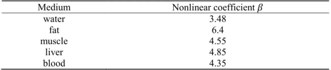
The nonlinear coefficient � for biological tissue falls in the range of 3 to 7 [Duck (1990)], while the contrast agents can have nonlinear coefficient of more than 1000 if the concentration is high [Wu et al. (1998)]. Table 3.1 lists the values of nonlinear coefficient for several different biological tissues.

Table 3.1 Value of nonlinear coefficient for several biological tissues

Medium Nonlinear coefficient �

water 3.48

fat 6.4

muscle 4.55

liver 4.85

blood 4.35

3.3.2 Lossless Burgers equation

The propagation of a plane wave in a lossless medium can be described by the lossless Burgers equation [Burgers (1948)]:

�� = �� 0�03 �� (3.14)

where � is the delayed time, � = � − � �⁄ . The solution of Eq.(3.14) was proposed by ₀ Fubini [Fubini (1935)]: �(�, �) = �0� 2 �� ∞ �=1 ��(��)sin (��0�) (3.15) where � is the number of harmonic, �_� is the Bessel function of ��ℎ order and �_� is the dimentionless distance, expressed as:

�� =�_�0��0 0�03 �

(3.16)

3.3.3 Complete Burgers equation

In reality, the ultrasound wave propagation has not only nonlinear effect, but also the absorption and dispersion effects. Because of these effects, some of the wave energy is converted in heat. So the wave energy is attenuated.

Taking into account the attenuation, the Burgers equation is expressed as: �� = �� 0�03 �� + � 2�₀3 �2_� ��2 (3.17)

(28)

3.3.4 KZK equation

Section 3.3.2 and section 3.3.3 consider a plane wave propagation, however in reality, transducers have finite size. So the diffraction effect should also be taken into account. The complete model of nonlinear wave propagation in a medium can be described by the Khokhlov-Zabolotskaya-Kuznetsov (KZK) equation [Zabolotskaya

et al. (1969); VP Kuznetsov (1970)]: �� = �0 2 ∆⊥� + � 2�₀3 �2_� ��2 + �� 0�03 �� (3.18)

where ∆_⊥� presents the diffraction effect of the transducer and depends on the transducer shape. The three terms in the right side of (3.18) stand for diffraction effect of the probe, the attenuation of the medium and the nonlinear distortion of the medium, respectively.

If the transducer is a circular single element transducer, as illustrated in Figure 3.2, then ∆⊥� = � (� 2_� ��2 + 1 � �� )��′ � −∞ (3.19) where � is the radius of the transducer.

If the transducer is a linear-array probe, as illustrated in Figure 3.3, then ∆⊥� = � (� 2_� ��2 + �2_� ��2)��′ � −∞ (3.20) The geometrical parameters of linear-array probes, which are important for the diffraction effect, are described in Figure 3.4 and listed below:

• ��: number of elements of the transducer

• ��ℎ: width of the element in the lateral direction � • ��ℎ�: height of the element in the elevation direction � • ��: spacing between two consecutive elements

(29)

Figure 3.2 Single element transducer

Figure 3.3 Linear array probe.

(30)

3.4 Simulators

Coupling with the study to nonlinear ultrasound propagation, various simulation tools have been developed. In this section, two simulators, used in this thesis, are introduced.

3.4.1 Voormolen simulator

The Voormolen is a nonlinear ultrasound propagation simulator, using a time domain algorithm as solution to KZK equation, for rectangular array with arbitrary excitation [Voormolen (2007)]. The impact of the different dimension of the array is taken into account. The different effects are solved with a finite difference scheme.

The time domain solution proposes a higher order in nonlinear interaction but needs a long computation time to converge to the solution. In order to decrease the computation time, the steps in the propagation direction are not equal, because more accuracy is required in the near field.

3.4.2 CREANUIS

CREANUIS is a tool that simulates nonlinear radio frequency (RF) ultrasound images containing both the fundamental and the second-harmonic evolution [Varray

et al. (2013)]. It is the combination of two specific tools. The first tool is a nonlinear

ultrasound propagation simulator that allows computing the increase of the fundamental and second-harmonic wave [Varray et al. (2011)]. The second tool is a reconstruction algorithm, using this field information and creating the corresponding nonlinear radio frequency (RF) image [Varray et al. (2010)].

For the nonlinear ultrasound propagation simulator, a generalized angular spectrum method (GASM) is used, so medium with an inhomogeneous nonlinear coefficient can be simulated.

3.5 Conclusion

In this chapter, the theoretical background about nonlinear wave propagation in biological tissue is mainly introduced. The development of new imaging techniques requires realistic conditions for simulated data. This chapter also shows that several tools can be used to simulate biological tissue when the nonlinearity of the medium is concerned.

(31)

(32)

Chapter 4

4. Generalization of multi-pulse transmission

4.1 Introduction ... 23 4.1.1 Single-pulse techniques ... 24 4.1.2 Multi-pulse techniques ... 25 4.2 Theory ... 27 4.2.1 Mathematical background ... 27 4.2.2 Application to several multi-pulse techniques ... 29 4.2.2.1 Pulse inversion (PI) and second harmonic inversion (SHI) ... 29 4.2.2.2 Amplitude modulation (AM) ... 30 4.2.2.3 Pulse inversion amplitude modulation (PIAM) ... 30 4.2.2.4 Phase-coded sequences (PCS) ... 31 4.2.2.5 Contrast pulse sequences (CPS) ... 31

4.3 Simulations and discussions ... 32 4.4 Conclusion ... 38

(33)

In order to increase the contrast-to-tissue ratio (CTR) in contrast imaging or the

signal-to-noise ratio (SNR) in tissue harmonic imaging, many multi-pulse transmission techniques have been proposed. This chapter presents a mathematical background to generalize most of the multi-pulse ultrasound imaging techniques. The presented formulation can be used to predict the nonlinear components in each frequency band. Simulation results on several multi-pulse techniques agree with the results given in previous literatures.

This chapter is the work presented in the journal article submitted to Ultrasonics [Lin et al., 2013b].

Ultrasound echography is now widely used for the diagnosis of many diseases because it is non-invasive, simple to implement and relatively low cost compared to other modalities. In conventional imaging, the amplitudes of the reflected echoes are detected and used to form a B-mode image. Following the use of ultrasound contrast agents (UCA), diverse imaging techniques appear. UCA are suspensions of micro-bubbles injected intravenously and pass through the lung capillary circulation. They are stable enough to avoid rapid disappearance. Most of them have diameters less than 10 µm. UCA are used to enhance the backscattered signal from the blood pool [Gramiak et al. (1968)]. It was found that bubbles also backscattered harmonics because they vibrated asymmetrically (expanding much more than compressing) when exposed to an ultrasound pulse [De Jong et al. (1994a), (1994b)]. Previously, tissue was considered as a linear reflector, especially under low acoustic power, so it was natural to adopt harmonic imaging, which filters out the harmonics of UCA, to observe the behaviour of blood flow in large vessels and myocardial and tumour perfusion, in contrast imaging [Porter et al. (2010)]. Second-harmonic imaging is the most common imaging used [Burns et al. (1992), (1996)].

Unfortunately, tissue can also generate harmonics because the transmitted wave is deformed gradually during its propagation in tissue [Aanonsen et al. (1984)]. Therefore, in ultrasound contrast imaging, the contrast-to-tissue ratio (CTR) is limited because of tissue-generated harmonics. CTR is used to quantify the extent of discrimination between UCA and tissue and can be defined at a specified ��ℎ harmonic:

�� = 20��

(4.1) where �_�� and �_�� are backscattered pressures of the ��ℎ harmonic from UCA and tissue, respectively.

In the other hand, harmonic imaging can be applied to tissue only, without injecting UCA, in order to improve resolution [Ward et al. (1997)], to increase the

(34)

signal-to-noise ratio (SNR) and to reduce artefacts. This technique is called tissue harmonic imaging [Bouakaz et al. (2003); Shen et al. (2007a), (2011)].

Besides the common criteria to judge the imaging quality of an ultrasound imaging technique, such as higher image resolution and fewer image artefacts, CTR is the main parameter in contrast imaging, and SNR in tissue harmonic imaging without UCA. Equation (4.1) claims that, to increase CTR in contrast imaging, the echoes generated by tissue should be reduced and those produced by UCA should be enhanced. In tissue harmonic imaging, conversely, the harmonic echoes from tissue should be enhanced while the other signals should be decreased.

4.1.1 Single-pulse techniques

Conventional B-mode imaging and second-harmonic imaging, including contrast harmonic imaging and tissue harmonic imaging, use a single-pulse transmission. In addition to these approaches, Forsberg et al. proposed sub-harmonic imaging by receiving at half of the transmitted frequency to increase CTR [Forsberg et al. (2000)]. Bouakaz et al. proposed super-harmonic imaging, transmitting at low frequency (0.8 MHz) and taking advantage of combined harmonics higher than third harmonics (third, fourth, fifth, …), termed super-harmonics, to increase CTR [Bouakaz et al. (2002)]. This method can also be used to image native tissue by transmitting at a higher frequency (1.2 MHz) to increase SNR [Bouakaz et al. (2003)].

Besides these techniques, several groups used the idea of source prebiasing to increase ��₂ by suppressing the second harmonic generated by tissue. The difference between these techniques lies in how the source prebiasing signal is designed. Krishnan et al. predicted the waveform at the focus and the source prebiasing signal is the inversion of the obtained second-harmonic signal mixed with the imaging pulse [S Krishnan et al. (1996), (1998); Christopher (1999); KB Krishnan

et al. (2008)]. This method was named the harmonic cancellation system (HCS).

However, the tissue harmonic is reduced over a narrow band and a limited range of axial field. Pasovic et al. eliminated this disadvantage by defining a multiple-frequency component second-harmonic prebiasing signal [Pasovic et al. (2010)]; this technique is called multiple-component second-harmonic reduction signal (mcSHRS).

Shen et al. proposed transmitting a fundamental and a phase-shifted third harmonic wave simultaneously. The second harmonic is decreased when the frequency-sum component and the frequency-difference component are out of phase. When the two components are in phase, the second harmonic is enhanced. Therefore, this technique can be used in contrast imaging as well as in tissue harmonic imaging [Shen et al. (2007b), (2008b)]. These authors also suggested using the harmonic leakage signal to generate the second-harmonic reduction signal [Shen et al. (2008a), (2010)].

(35)

4.1.2 Multi-pulse techniques

However, in conventional harmonic imaging, the following problem is always encountered: if a short pulse, that is a broadband pulse, is transmitted, there is an inevitable spectral overlap between the fundamental and harmonic frequencies. To increase the sensitivity of the system in detecting harmonic echoes, a multiple-cycle pulse, that is a narrowband pulse, has to be transmitted, which unfortunately causes the a deterioration of the imaging resolution [Frinking et al. (2000); Chiao et al. (2003)].

To overcome the trade-off between contrast detectability and imaging resolution in conventional harmonic imaging and to further explore the specific ultrasonic properties of micro-bubbles as well as those of tissue, many multi-pulse techniques have been developed. Most of them modulate the transmission and reception frequency, pulse amplitude, pulse phase, pulse duration, number of pulses, pulse repetition frequency (PRF) and so on.

In pulse inversion (PI), a sequence of two inverted pulses is transmitted [Hwang (1999); Simpson et al. (1999)]. For a linear system, the response to the second pulse is an inverted copy of the response to the first one and the sum of the two responses is zero. For a non-linear system, the sum is not zero. Pulse inversion works over the entire bandwidth of the received echo signal and achieves better image resolution.

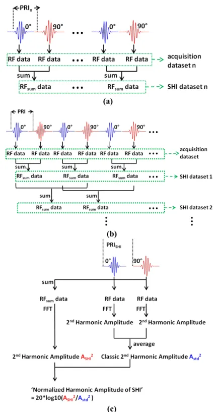
To suppress tissue harmonics in contrast imaging, Couture et al. developed PI using time reversal [Couture et al. (2008)]. The backscattered echoes from two inverted pulses were time-reversed and then used as excitation pulses. The echoes received from the new excitation signals were summed to form an image. Pasovic et al. proposed a method called second-harmonic inversion (SHI)1 [Pasovic et al. (2011)]. As in PI, a sequence of two pulses is transmitted and the two responses are summed, but the phase shift between the two transmitted pulses is 90°. Because the second-harmonic component has a quadratic relationship to the fundamental one, the phase shift between the two second-harmonic components is 180°, so the second harmonic is cancelled successfully in tissue. In the contrast agent region, good preservation of the second harmonic was observed (maximum reduction was only 0.3 dB), therefore, the CTR is effectively increased. The preservation of the second harmonic was explained when Morgan observed that the signals reflected from a single bubble excited by two inverted one-cycle pulses have frequency shift and that the polarity of the two echoes received is not significantly changed [Morgan et al. (1998)].

1

SHI refers to second-harmonic imaging, sub-harmonic imaging [Forsberg et al. (2000)], super-harmonic imaging [Bouakaz et al. (2002)] or second-harmonic inversion [Pasovic et al. (2011)] in different literatures.

(36)

There are also several methods to increase the non-linear response of microbubbles. Borsboom et al. proposed a method called pulse subtraction time delay imaging. Three pulses were transmitted. The third pulse emitted was the juxtaposition of the first two non-overlapping pulses. The echoes from the first two pulses were subtracted from the echo from the third pulse [Borsboom et al. (2009)]. Brock-Fisher et al. used a modulation in amplitude (AM) [Brock-Fisher et al. (1996)]. The linear echoes were cancelled but the odd nonlinear components were preserved. The combination of phase and amplitude modulation in a more generalized non-linear detection process was first suggested by Haider and Chiao [Haider et al. (1999)]. Phillips further evaluated this idea for three different UCA with several sequences called contrast pulse sequences (CPS) [PJ Phillips (2001); P Phillips et al. (2004)]. Eckersley et al. [Eckersley et al. (2005)] combined PI and AM where the second pulse was inverted and its amplitude was half that of the first pulse. The response to the second pulse was multiplied by two before being summed with the response to the first pulse. CTR was enhanced by 4±1 dB. Wilkening et al. transmitted five pulses with equidistant phases, a weighted summation of the received echoes suppressed the selected harmonics [Wilkening et al. (2000), (2001)].

There are also some multi-pulse techniques using different threads. Frinking et al. transmitted identical imaging pulses separated by a release burst which partially destroyed the UCA. The presence of UCA was detected by correlating or subtracting the response of the imaging pulses before and after the release of free gas bubbles [Frinking et al. (2001)]. Reddy et al. also used pulse inversion to increase the response of bubbles by identifying the shape of the driving pulse with limited driving intensity [Reddy et al. (2002)]. A dual-pulse frequency-compounding (DPFC) method was proposed to reduce the ghost reflection artefacts in super-harmonic images. Each radio frequency (RF) line is the summation of the response from two transmissions with slightly different centre frequencies [Van Neer et al. (2011)].

To eliminate the non-linear components produced by capacitive micromachined ultrasonic transducers (CMUTs), Novell et al. proposed two methods: one of them transmits the inverse signal of the undesired harmonic component while the other uses the interaction between the fundamental component and the selected transmitted frequency component to cancel the undesired harmonic component [Novell et al. (2009)].

Besides the imaging techniques mentioned, Doppler techniques, used to measure the blood flow, can be considered as multi-pulse techniques. Conventional pulsed Doppler and colour Doppler techniques repeat the same pulse for each line to track the moving scatterers in a region of interest (ROI); the movement then represents blood velocity. Power Doppler displays the power of the Doppler signal instead of the flow velocity. The Doppler technique has also been combined with harmonic imaging

(37)

leading to harmonic power Doppler (HPD) [Burns et al. (1994)] in order to increase the detectability of bloods or combined with PI to give the technique called pulse inversion Doppler (PID) [Simpson et al. (1999)] to decrease tissue movement artefacts. The pulse subtraction Doppler (PSD) was developed to differentiate bubble motion from tissue motion [Mahue et al. (2011)].

This chapter aims to present a generalized mathematical background to generalize most of the multi-pulse techniques in ultrasound imaging. The formulation obtained fits with previously proposed techniques to increase or to decrease specified nonlinear components in a specified harmonic band. Simulation results are shown to verify the generalization of this formulation and demonstrate that most of the nonlinear imaging techniques can be generalized by this formulation. The organization of the chapter is as follows. Section 4.2 introduces the theoretical background. Examples of several techniques are presented using the proposed formulation. The simulation results of several multi-pulse transmission techniques are shown and discussed in Section 4.3, to verify the generalization of such a mathematical background for multi-pulse transmissions. Section 4.4 concludes this chapter.

4.2 Theory

4.2.1 Mathematical background

When a wave propagates in a non-linear medium, the wave is deformed gradually during the propagation because of the diffraction effect of the probe, the absorption of the medium and the non-linear distortion of the medium [Aanonsen et al. (1984)]. Assuming the transmitted acoustic wave is:

�0(�) = �0��0�+�0 (4.2)

where �₀ is the amplitude of the wave, �₀ is the angular frequency and �₀ is the phase. The received wave �(�) is modelled as the polynomial expansion of a basis waveform �₀ [Haider et al. (1999)]:

�(�) = �1�0(�) + �2�02(�) + ⋯ + ��0�(�) = � ��0�(�) �

�=1

(4.3) where �₀ is the basis waveform for the nonlinear components, �_� is the weight of the ��ℎ_{-order nonlinear component,}_{� is the presumed model order. The expression of �}

� and �₀ are not detailed here. �_� is a complex term depending on the medium (tissue or bubbles) and on the frequency and amplitude of the transmitted wave. The waveform �0 also depends on the transmitted wave �0. In a linear system, only �1 would be nonzero.

(38)

�0(�):

�02(�):

�03(�):

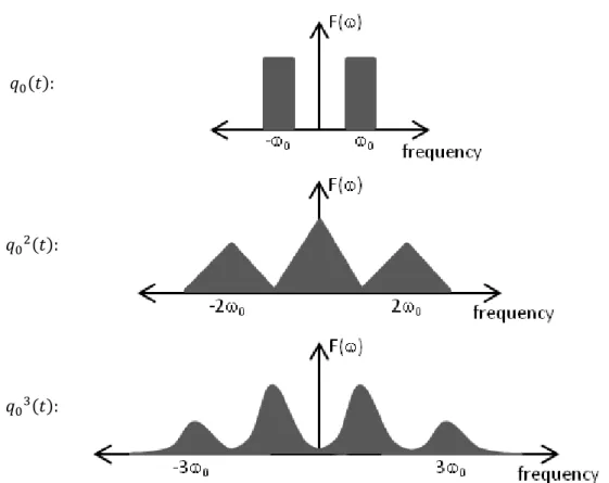
Figure 4.1 Demonstration of �-times auto-convolution of the spectrum of the linear term �0 (after Haider et al. (1999)).

As Figure 4.1 shows, in the frequency domain, the time domain multiplication �₀� in Eq. (4.3) becomes �-times auto-convolution of the spectrum of the linear term �₀ (centred in �₀), this repeated convolution results in not only the spectrum component of the frequency band centred in ��₀, but also spectrum components of lower frequency band. In other words, the final signal level of the ��ℎ frequency band is decided by not only the ��ℎ-order nonlinear component, but also the higher order nonlinear components. In general, odd-order nonlinear components in (4.3) create spectrum components at odd multiples of �₀, while even-order nonlinear components create spectral components at even multiples of �₀ [Haider et al. (1999); Eckersley et

al. (2005)].

This property implies that the specific nonlinear component in one frequency band could be increased or decreased using pulse transmission techniques. In multi-pulse transmission techniques, multi-pulses are transmitted successively. Equation (4.2) is rewritten as the basic waveform of the transmitted pulses:

�0(�) = �0��0�+�0 (4.4)

Suppose � pulses are transmitted into the medium and �_� indicates the relationship between the ��ℎ transmitted pulse �_� and the basic waveform �₀ [Haider et al. (1999)]:

(39)

��(�) = ��0��0�+�0 (4.5) �� = |��|��, ��[0,2�], � = 1,2, … , � (4.6) Then after propagating some distance in the medium and back-propagating to the probe, the pulses are received and multiplied by a weighting vector �_� before being added together. The summation of these received pulses can be expressed as:

��(�) = � �� 0�(�) � �=1 � � �=1 (4.7) Equation (4.7) is the general expression of the sum of � pulses propagating some distance and going back. The enhancement or cancellation of selective nonlinear components depends on the choice of coefficient vector � and �:

� = (�1, … ,��) (4.8)

� = (�1, … ,��) (4.9)

To clearly see the dependence of each nonlinear components on the coefficient vector � and �, (4.7) is written as:

��(�) = � �� =1 � ��0�(�) � �=1 (4.10) so the weight of the ��ℎ nonlinear component in the final summed signal is:

� �� =1

(4.11) These assumptions will be validated, in the latter part of this chapter, through the comparison between simulation results presented in this chapter and experimental results from previous literature.

4.2.2 Application to several multi-pulse techniques

In the following section, the formulation (4.10) is applied to several techniques presented in section 4.1. For simplicity and effective comparison, the first transmission and reception are regulated to be the same for all the following multi-pulse techniques, that is, �₁ =�₁ = 1. In all the cases presented in the present chapter, the fundamental and second-harmonic frequency bands are concerned, so only the linear component and third-order nonlinear component contributing to the fundamental band and the second-order nonlinear component contributing to the second-harmonic band are calculated, meaning that the presumed model order is � = 3.

4.2.2.1 Pulse inversion (PI) and second harmonic inversion (SHI)

For double-pulse transmissions such as PI and SHI, �₂ defines the phase shift between the two transmitted pulses.

(40)

��= �1, ��2�

� = (1,1) (4.12)

For PI, �₂ =�, substituting (4.12) into (4.10), the summation can be written as: ��(�) = ��1 + ��0�(�)

� �=1

(4.13) Therefore, when � is odd, �� =−1; when � is even, ��= 1. That is, every odd nonlinear component is zero and every even nonlinear component doubles.

Similarly, for SHI [Pasovic et al. (2011)], �₂ = �

2, so the summation (4.10) is: ��(�) = � �1 + ��2� ��0�(�)

� �=1

(4.14) Therefore, when � = 4� + 2 (� = 0,1,2 … ), ��2 ₌−1 . That is, every (4� + 2 )�ℎ nonlinear component is zero.

4.2.2.2 Amplitude modulation (AM)

In the technique AM described by Brock-Fisher et al. [Brock-Fisher et al. (1996)], � is a real vector. � �=�1, 1 2� � = (1, −2) (4.15) substituting (4.15) into (4.10), the summation becomes:

��(�) = �(1 − 21−�)��0�(�) � �=1 (4.16) Therefore, (4.16) becomes: ��(�) = 0 + 0.5�2�02(�) + 0.75�3�03(�) (4.17) Equation (4.17) illustrates the linear component is cancelled in AM technique; the third-order nonlinear component, which also contributes to the signal level of the fundamental frequency band, becomes 0.75 times compared to one single transmission (refer to (4.3)) and the second-order nonlinear component becomes 0.5 times compared to one single transmission.

4.2.2.3 Pulse inversion amplitude modulation (PIAM)

In the technique proposed by Eckersley et al. [Eckersley et al. (2005)], the pulse inversion and amplitude modulation were combined.

��= �1, ��

2 � � = (1,2)

(4.18) substituting (4.18) into (4.10), the summation becomes:

(41)

��(�) = ��1 + 21−��0�(�) � �=1 (4.19) For � = 3, (4.19) becomes: ��(�) = 0 + 1.5�2�02(�) + 0.75�3�03(�) (4.20) Compared to the AM technique, the linear component in PIAM technique is also cancelled; the third-order nonlinear component, which contributes to the signal level of the fundamental frequency band, remains the same; but the second-order nonlinear component is larger.

4.2.2.4 Phase-coded sequences (PCS)

For the phase-coded sequences (PCS) technique described in [Wilkening et al. (2000)], five transmissions with equidistant phases are transmitted. Subsets with three transmissions are investigated to cancel the linear component but to preserve the second-order and third-order nonlinear components in the fundamental frequency band. The parameters � and � for the three transmissions in the subsets are:

⎩ ⎪ ⎨ ⎪ ⎧ � = �1, ��2�5,�−�2�5 � � = �1, − 1 2 cos2₅� ,− 1 2 cos2₅� � (4.21) substituting (4.21) into (4.10), ��(�) = � �1 −� �2��₅ ₊_�−�2��₅ 2 cos2₅� � ��0�(�) � �=1 (4.22) For � = 3, (4.22) becomes: ��(�) = 0 + �1 − cos(4� 5⁄ ) cos(2� 5⁄ )� �2�0 2₍_{�) + �1 −}cos(6� 5⁄ ) cos(2� 5⁄ )� �3�0 3₍_�) = 0 + 3.618�₂�₀2(�) + 3.618�₂�₀2(�) (4.23) Equation (4.23) shows the linear component is also cancelled in PCS technique; the third-order nonlinear component, which also contributes to the signal level of the fundamental frequency band, becomes 3.618 times compared to one single transmission (refer to (4.3)) and the second-order nonlinear component also becomes 3.618 times compared to one single transmission.

4.2.2.5 Contrast pulse sequences (CPS)

In [PJ Phillips (2001)], eight groups of sequences called contrast pulse sequences were evaluated. For each group, selective nonlinear components are emphasized after the cooperation of � and �. The eight sequences are listed in Table 4.1.

(42)

��= �1, �� 2 , 1 2,� ��_� � = (1,2, −2, −1) (4.24) substituting (4.24) into (4.10), ��(�) = ��(21−�− 1)��− 1��0�(�) � �=1 (4.25) For � = 3, (4.25) becomes: ��(�) = 0 + 0 + 1.5�3�03(�) (4.26)

Therefore, the linear component and the second-order nonlinear component are cancelled while the third-order nonlinear component is 1.5 times compared to the single transmission (refer to (4.3)).

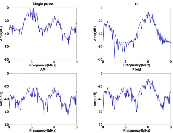
4.3 Simulations and discussions

To verify the generalization of the formulation, simulations for several multi-pulse techniques, namely SHI [Pasovic et al. (2011)], PI [Hwang (1999); Simpson et al. (1999)], AM [Brock-Fisher et al. (1996)], PIAM [Eckersley et al. (2005)], PCS [Wilkening et al. (2000)] and CPS [PJ Phillips (2001)], were conducted. Considering the experimental results have already been well presented in the mentioned literatures, only simulations were conducted. The validation of this mathematical background was done by comparing these simulation results with the previously published experimental results described in the literature.

A simulation tool, based on a finite difference method proposed by Voormolen to solve the KZK wave propagation equation, was used [Voormolen (2007)]. The harmonic images were computed with a delay and sum algorithm as proposed in CREANUIS software [Varray et al. (2010), (2013)]. The dimensions used for simulation of pressure field were listed in Table 4.1. UCA were considered as a non-linear medium with a higher coefficient of nonnon-linearity � and a stronger reflectivity than tissue. The UCA region was simulated as a tube with a diameter of 8 mm and a tilt angle of 35°. The image depth was 100 mm. The tissue region was also considered as a non-linear medium, which is realistic, instead of a linear medium considered in most of the multi-pulse contrast imaging techniques.

The coefficient of nonlinearity � of tissue and UCA were set according to the values of nonlinear parameter � �⁄ reported in previous literatures. The � �⁄ of the biological media was measured to be approximately in the range of 6 and 10 [Zhang

et al. (1999), (2001)]. Then considering � equals to 1 + � 2�⁄ , � value was from 4 to

6. The coefficient of nonlinearity � of tissue was set as 4.5. The � �⁄ of two contrast agent (Albunex and Levovist) were measured to be an increasing function of bubble number densities [Wu et al. (1998)]. In our simulation, the coefficient of