HAL Id: hal-01869813
https://hal.univ-lorraine.fr/hal-01869813
Submitted on 6 Sep 2018
HAL is a multi-disciplinary open access
archive for the deposit and dissemination of sci-entific research documents, whether they are pub-lished or not. The documents may come from teaching and research institutions in France or abroad, or from public or private research centers.
L’archive ouverte pluridisciplinaire HAL, est destinée au dépôt et à la diffusion de documents scientifiques de niveau recherche, publiés ou non, émanant des établissements d’enseignement et de recherche français ou étrangers, des laboratoires publics ou privés.
The influence of spring geophytes on soil CO2 efflux in a
Common beech forest
Laura Heid
To cite this version:
Laura Heid. The influence of spring geophytes on soil CO2 efflux in a Common beech forest. Sciences de l’environnement. 2012. �hal-01869813�
AVERTISSEMENT
Ce document est le fruit d'un long travail approuvé par le jury de
soutenance et mis à disposition de l'ensemble de la
communauté universitaire élargie.
Il est soumis à la propriété intellectuelle de l'auteur. Ceci
implique une obligation de citation et de référencement lors de
l’utilisation de ce document.
D'autre part, toute contrefaçon, plagiat, reproduction illicite
encourt une poursuite pénale.
Contact : [email protected]
LIENS
Code de la Propriété Intellectuelle. articles L 122. 4
Code de la Propriété Intellectuelle. articles L 335.2- L 335.10
http://www.cfcopies.com/V2/leg/leg_droi.php
MASTER FAGE
Biologie et Ecologie pour la Forêt, l’Agronomie et
l’Environnement
Spécialité
FGE
The influence of spring geophytes on soil CO
2
efflux in a Common beech forest
Laura Heid
Mémoire de stage, soutenu à Nancy le 03/09/2012
Tuteur de stage: Stephan Glatzel, Professor
Responsable universitaire : Bernard Amiaud, Lecturer
Structure d’accueil :
Chair for Landscape Ecology and Site Evaluation
University of Rostock
Justus-von-Liebig Weg 6, Rostock, Germany
Acknowledgement
&
First of all I wanted to thank Pr. Stephan Glatzel who welcomed me into his unit and allowed me to expand my vision of the scientific world. Thank to him and Dr. Gerald Jurasinski for giving me such an interesting subject. Thanks for your (R-) help, advice, reading, correction,… Thanks for giving me the opportunity to improve (myself) and to get to see what it means to be a scientist!
I want to thank particularly Franziska Koebsch who helped me survive in Rostock, in nearly every aspect of my life there (scientific or not), thanks for all your advice and for our (always) serious talks, and of course I could not thank you enough for having showed me the joy of your field work! A big thank to Sascha Beetz for his unbelievable patience with me and my several EGM and electrical problems and for his interest in my results. And thanks to Marian Koch for his implication in my study and his help when I thought it started to get unmanageable and hopeless (and for correction, motivation and tons of other things)! As promised back then to you two Marian and Sascha, thanks for helping setting up the site!
Thanks to all of the Ph.D. students (German or Taiwanese) for their help on practical problem, on lending soil probe, digging soil profiles,…
And thanks again to all the member of the chair that I (probably) bothered during their work several time, thanks a lot for your help (on scientific or administrative matter)! And thanks to all the people who have contributed to this study (without forgetting the students of the Master program “Environmental Engineering” for their hard work)!
Table of Contents
&
INTRODUCTION ... 2
MATERIAL AND METHODS ... 4
SITE DESCRIPTION: ... 4
SOIL CO2 EFFLUX: ... 5
ADDITIONAL MEASUREMENTS: ... 5
Soil climatic related parameters ... 5
Soil study ... 6
Vegetation survey and spots’ geolocalisation: ... 6
RELATIVE FINE ROOT BIOMASS ... 6
DATA MANAGEMENT AND ANALYSIS: ... 7
Soil CO2 efflux ... 7
Soil CO2 efflux modeling ... 7
Statistical analysis ... 8
Mapping ... 8
RESULTS ... 9
SEASONAL VARIATION OF THE SOIL CO2 EFFLUX ... 9
SPATIAL VARIATION OF THE SOIL CO2 EFFLUX: ... 11
COMPARISON BETWEEN G SPOTS AND NG SPOTS: ... 13
SOIL CO2 EFFLUX AND RFRB: ... 16
DISCUSSION ... 17
SEASONAL VARIATION AND RELATIONSHIP WITH SOIL TEMPERATURE: ... 17
ROLE OF THE GEOPHYTES: ... 17
LINK BETWEEN SOIL CO2 EFFLUX AND RFRB: ... 18
CONCLUSION ... 19
BIBLIOGRAPHY ... 20
1
Abbreviations
S C: Carbon
C:N ratio: Ratio between the Carbon and Nitrogen content dbh: Diameter at Breast Height
FRB: Fine Root Biomass G: Geophytes
GHG: Greenhouse Gases
GIS: Geographic Information System GPP: Gross Primary Production IRGA: Infra-Red Gas Analyzer N: Nitrogen
NEE: Net Ecosystem Exchange NG: Non-Geophytes
PCC: Pearson’s correlation coefficient
Reco: Ecosystem respiration
Rs: Soil respiration
rFRB: relative fine root biomass RSS: Residual Sum of Square ST: Soil Temperature
SWC: Soil Water Content
Figures and tables
&
Figure 1: The carbon balance of a forest
Figure 2: Location of the study site, (Rostocker Heide, Rostock, Germany) Figure 3: Dispersion and orientation of the transects
Figure 4: Mean soil CO2 efflux, mean soil temperature at 10 cm and mean SWC Figure 5: Soil CO2 efflux per transect
Figure 6: Map of the mean soil CO2 efflux and the soil seasonal modeled CO2 emissions
Figure 7: Difference between either the modeled seasonal emissions or the mean soil efflux and the
presence of Geophytes in the spots or not
Figure 8: Correlation between N content, C content and C:N ratio and a mean value of the measured
soil CO2 value
Figure 9: N content and C content in per cent and C:N ratio of the soil for G and NG spot Figure 10: Mean soil CO2 efflux and Seasonal soil emissions related to the rFRB
Figure 11: Difference between G and NG spots according to several definitions
Table 1: Values of the constant t1, the activation energy (E0) and the residuals sum of square (RSS)
Table 2: Modeled seasonal coil CO2 efflux mean values of geophytes and non-geophytes spots
Table 3: Soil CO2 efflux range from other studies
2
Introduction
1 The faculty of Agricultural and Environmental Sciences, founded in 1942, is one of the nine faculties of the University of Rostock, Germany. Among the 20 chairs, stand the Landscape Ecology and Site Evaluation where I have done my training. The goal of this chair is to try to understand to what extent the matter and greenhouse gas balance of a site, an ecosystem or a landscape is driven by vegetation and/or soil and other environmental parameters.
It has been shown that the CO2 concentrations have increased in the atmosphere
since the beginning of industrialization (IPCC, 2007; Revelle et al., 1957). CO2 acts as a
greenhouse gas (GHG) and because its release has increase dramatically it is the principal driver of global warming (Cox et al., 2000). In the context of global change and climate warming it is important to better understand the carbon cycle and the rate of exchange of carbon in every ecosystem. Some ecosystems are described as ‘carbon sinks’ because they keep more carbon than they release. That is why the carbon increase in the atmosphere could be limited by storage in these ecosystems.
Vegetation is an important terrestrial carbon sink, thanks to photosynthesis. The carbon is stored in the plant until either the leaves fall or a part of the plant dies. Then the plant matter is decomposed to CO2 or partially passed into the soil. Forests are among the
important terrestrial carbon sinks; they store 30% of the GHG emitted worldwide (Service de l’observation et des statistiques, 2011). Therefore, in recent years researchers focused on widening our understanding of the carbon cycle and on quantifying the actual carbon balance (Figure 1) in terrestrial ecosystems.
Figure 1: The carbon balance of a forest is the result from the difference between GPP (Photosynthesis) and Reco (carbon release or respiration). Reco is made up of two terms, plant respiration (Rplant) and soil respiration (Rs)
Soil respiration is the most important term of ecosystem respiration. It has been shown that it can amount to up to 70% of Reco in European broad-leaved forest (Granier et
3
al., 2000; Valentini et al., 2000). Rs can be divided further into autotrophic and heterotrophic
respiration. Autotrophic (or root) respiration is realized by living roots and the associated microorganismic respiration whereas heterotrophic (or microbial) respiration stems from microorganisms that live directly in the soil. But the separation between the two is challenging. The available methods to do so (trenching, girdling) considerably modify the environmental properties (Epron et al, 1999b; Hanson et al., 2000). After all, root respiration seems to represent an important part of soil respiration, but available studies show great variation. Hanson et al. reviewed the literature in this regard and report shares of root respiration on soil respiration from 10% to 90%. In a beech forest in north east France (Epron et al., 1999b and 2001) about 60% of the total soil respiration came from roots.
The problem for share studies is that soil respiration varies considerably in space and time. This variability depends on three groups of factors: edaphic factors like soil’s texture and structure; biological factors like vegetation type, litter’s quality and quantity (Longdoz et al., 2000; Fang et al., 1998), and climatic factors like temperature (Longdoz et al., 2000) and soil humidity (Epron et al., 1999a). Several authors have therefore tried to model soil respiration using these factors.
Jurasinski et al. (2012), used tree fine root biomass (FRB) as a proxy in the modeling of soil respiration patterns. The estimated FRB of Ash (Fraxinus excelsior) explained some variation in measured CO2-efflux of an old-growth forest in Central Germany. Yet, the
modeled tree FRB from other species (Fagus sylvatica for example) could not be used to model soil respiration. A possible explanation was that the activity of spring geophytes might mask the direct effect of the tree fine roots, due to high springtime heterotrophic respiration.
Geophytes are plants able to survive the cold season thanks to their perennating buds that lay in underground storage organs (bulb, rhizome...) (Dafni et al., 1981). Thanks to this specificity, geophytes develop themselves as soon as the conditions (light, temperature, humidity) are propitious again after the dormant season. They are present in a large panel of habitat, from grasslands (like Muscari tenuiflorum) to forests (Anemone nemorosa for example) where they are the first to bloom, forming a grassy expanse on the forest’s soil. Depending on biom and species, they grow in different seasons (early spring, summer...).
Geophytes constitute an important floristic element of European beech forests (Ellenberg and Leuschner, 2010). They are generally found in forests on soils with intermediate pH and nitrogen availabilities, mild temperatures and medium humidity (Hermy et al., 1999; Morschhauser et al., 2009; Hermann et al., 2005). They typically grow in patches. The conditions for their presence are not yet well known. Morschhauser et al., (2009) suggested that the establishment of Allium ursinum depends on the neighbor density; more precisely the establishment was better in stands of intermediate plant density. However, despite their importance on the forest floor, little is known about their possible impact on soil respiration.
4 During my internship, I studied both the role of springtime geophytes on the soil respiration in a beech forest and the possible correlation of soil CO2 efflux with the modeled
relative FRB using the model described in Jurasinski et al, (2012) work. The main purpose was to see whether the geophytes could modify the soil properties and the soil CO2 efflux
behavior of the forest.
Carbon turnover was expected to be faster during spring and early summer in parts of the ground where geophytes grow, leading to an increase in soil CO2 efflux. I tested the
hypothesis that soil respiration is higher in geophyte spots than in spots without visible geophytes but with similar environmental characteristics.
Material and methods
&
Site description:
The research has been carried in the “Rostocker Heide”; more precisely in the forest district Schnatermann, located in the North-East of Rostock (Germany; Figure 2). The forest in the study site is mainly composed of European beech (Fagus sylvatica). Other important species are Hornbeam (Carpinus betulus), European Ash (Fraxinus excelsior) and Sycamore maple (Acer pseudoplatanus). During the measurement period the ground vegetation consisted mainly of geophytes, particularly Anemone nemorosa and Ranunculus ficaria at the beginning of the study, and Galium odoratum in late spring. The soil at the study site is a Humic gleysol or an Umbrisol according to the F.A.O classification.
Study site
5
Soil CO2 efflux:
Soil CO2 efflux was measured from February to end of June, at least once every week. The 60
measurement locations (spots in the following) were arranged along 12 transects. Each of the 30 m long transects had 5 measurement locations equally. The spots were marked by permanently installed collars (diameter = 10 cm; height = 7cm). The collars were installed some weeks before the measurements started to avoid perturbation of the soil during measurements. We planned to set up the single transects in a specific position and direction so that each transect should stretch from inside a geophyte patch to adjacent, geophyte free areas of the forest floor while keeping soil environmental conditions similar and having the transects run in different, random directions to avoid bias from micro-climatic forces (see Figure 3). One transect was set up in a part of the forest where trees were cut recently. However, the site was set up in early February. Therefore, the geophyte patches were not easy to distinguish and when spring arrived it was clear that not all transect covered geophytes/non-geophytes as planned. Finally, a spot was considered as a geophyte (G) spot when there were geophytes growing inside the collar (36 spots) and as non-geophyte (NG) spot when there weren’t any geophytes growing inside the collar (24 spots). The collars were secured with 3 tent pegs to avoid removal by animals.
Soil respiration was measured with a portable, dynamic closed chamber system (SRC-1) equipped with an infra-red gas analyzer (IRGA, EGM4, both the chamber and the IRGA by PP-Systems, Hitchin, UK).
Additional measurements:
Soil climatic related parameters
Soil temperature was measured using 6 HOBO Data Loggers (Pendant temp/light, UA-002-64, Onset Computer Corp., Bourne, MA) placed near some of the transects (Figure 3) at 10 cm depth. They recorded temperature continuously during the length of the experiment, from the 18/02/2012 to 17/07/2012 and stored half hourly means. Additionally, during soil CO2 efflux measurement campaigns, at each spot I measured soil temperature at different
depths (2, 5 and 10 cm) and soil moisture with frequency domain reflectometry using a
Figure 3:Dispersion and orientation of the transects. The white dots represent the collars and the yellow ones the localization of the temperature logger
6 ThetaProbe Soil Moisture Sensor Type ML-2x and a Soil Moisture Meter-HH2 (AT-Delta-T Devices Ltd., Cambridge, UK).
Soil study
Two soil profiles have been dug on the site, one inside a patch and the other outside. The location was decided randomly on the site. Soil samples were taken once near each collar using a core cutter of known volume (100mL) by students from the University during a field course in the Master program “Environmental Engineering”. A cube of soil from the A horizon (after removing litter) of approximately 20 cm edge length was taken out with a spade and one core cutter sample was taken from the top (0-10 cm) and another was taken from the bottom (10-20 cm) of that cube. The core cutter samples were weighed, and then dried for 24 hours at 105°C in a drying oven (Binder, Tuttlingen, Germany). This allowed for calculating the soil bulk density at each collar, knowing the volume of soil that was taken. Then the total carbon and nitrogen contents of the samples were measured using an Elementar Analyzer (VarioMAX; Elementar Analysensystem Gmbh, Hanau, Germany). From Ctot and Ntot the C:N ratio of the samples was calculated giving an idea of the speed of
organic matter decomposition and of the quality of the soil. Vegetation survey and plot localization:
The vegetation was surveyed at the end of May by students of the University of Rostock during a field course in the Master program “Environmental Engineering”. Within one meter radius around the spot centre, all species and their respective cover were recorded. Further, the locations (x, y, z) of all collars and all trees in the vicinity of the transects were recorded using a tachymeter/total station (Leica TC600; Leica Geosystems, Munich, Germany). Further, the tree species and the dbh (diameter at breast height) of each tree were recorded.
Relative fine root biomass
Relative fine root biomass (rFRB) at each transect has been estimated using a heuristic model from Ammer and Wagner (2005) adapted to broad leaved tree species by Jurasinski et al. (2012). This model is, for any point in a system of x-y-coordinates, based on only two parameters: the distance from that point to a surrounding tree and its diameter at breast height (dbh). There are several assumptions for that model:
- The maximum extension of fine roots away from the trunk depends on the dimensions of the tree and exceeds the crown-covered area.
- The FRB decreases with the distance from the trunk - The FRB increases with dbh
- The maximum FRB can be found at a specific distance from the trunk.
To develop their model, Jurasinski et al. followed model A from Ammer and Wagner (2005) as the fit to measured FRB was better.
To calculate the rFRB the following equations have been used: - If D≥RD3, rFRB=0
7 If D<RD3, rFRB of a tree at point x,y is calculated
With: D the distance between the tree’s trunk and the position of the respective point, RD3=dbh/6; the maximum distance in meters, RD2 and RD1 represent 2/3 and 1/3
respectively of RD3, RD0 marks the trunk. rFRB0=dbh/40; rFRB1=0.83*rFRB0;
rFRB2=0.43*rFRB0 and rFRB3=0 where rFRB1, rFRB2 and rFRB3 are rFRB at distance
RD1, RD2 and RD3 (Parameterization is for beech and was directly taken from
Jurasinski et al. 2012).
Data management and Analysis:
Soil CO2 efflux
The CO2 efflux rate was calculated directly by the EGM-4, from the change of CO2
concentration within the chamber. To avoid outliers, the first and last decile from the total dataset has been removed.
Soil CO2 efflux modeling
It is current knowledge that soil CO2 efflux has a strong relationship with temperature
(particularly with the soil temperature at 10cm depth; Borken et al., 2002), that’s why the modeling has been based on this parameter. To find the best model fitting our data and their relationship to temperature, the function ‘reco’ (package ‘flux’; Jurasinski & Koebsch, 2012) was used. That function can test and fit the most Reco models (linear, exponential,…) used in
literature. After trying out several models, the Arrhenius function (Lloyd&Taylor, 1994) has been selected. It showed the lowest Residual Sum of Squares (RSS) and Akaike information criterion of all compared models and so provided the best fit for the majority of the transects.
(Equation 1)
With: R the estimated soil CO2 efflux at 10 cm depth (g m-2 h-1), T the soil temperature at 10
cm (°C), t1 a constant, E0 the activation energy (J mol-1), TRef the reference value (set
8 The model was fit to the soil CO2 efflux and soil temperature data separated into geophyte
and non-geophyte spots of each transect and the parameters t1 and E0 were determined.
Thus, we ended up with 2 different sets of model parameters for each transect. Knowing the soil temperature at 10 cm (from the Hobo measurements, these have been synchronized to hourly values by averaging the two subsequent half-hourly values from the loggers), we were able to estimate the soil CO2 efflux for each transect and each hour during the study
period using the equation and the respective model parameters. Hobo measurements were always taken for the transect closest to the loggers. Data gaps in two loggers were closed by constructing a model with the best fitting other logger data with complete coverage and using these data to predict the missing data at the logger with the incomplete data series. “Seasonal” CO2 emissions for the study period (February to June) were estimated by simply
summing up the modeled hourly fluxes for each transect and treatment (geophytes / non-geophytes). The same method has been applied to soil CO2 efflux data from each spot. In
this case the models were constructed and the parameters were fit per spot. Statistical analysis
We tested for statistical difference between G and NG spots for either the measured values using Man-Whitney’s non parametrical test for two samples as the distribution of the measured soil CO2 values wasn’t normal. The variances between the modeled seasonal
estimates of G and NG spots were tested with an ANOVA after checking for normality of the values.
To find a correlation between the soil C content, N content, C:N ratio and the soil CO2 efflux,
the Pearson’s correlation coefficient (PCC)- that gives a measure (between -1 and 1, meaning negative or positive correlation) of the strength of linear dependence between two variables - was calculated. The significance of the difference between these characteristics and the geophytes presence in the spot was assessed with Kruskal-Wallis test.
The PCC between the rFRB and the soil CO2 efflux (measured and estimated for the season)
was calculated in order to find a correlation.
All statistical analyses were carried out in R (R Development Core Team, 2012). Mapping
Several maps have been constructed with the free GIS software Quantum GIS ‘Lisboa’. The map of the estimated seasonal CO2 emissions at each collar was realized using the sum of
the modeled values calculated for each days of the measurement period. An average of the measured value at each collar has been mapped too.
9
Results
&
Seasonal variation of the soil CO2 efflux
From February to June, an evolution in soil CO2 efflux, soil temperature (ST) and soil water
content (SWC) has been observed (Figure 4). The daily average values of soil CO2 efflux
varied from 0.01 g.m-2.hr-1 (in March with a soil temperature at 10 cm of 4.35°C) to 0.91 g.m
-2
.hr-1 (in June, 9.15°C).
This change seems to follow the soil temperature evolution during the measurement campaign. We can see for example on May, 10th that the soil temperature reaches a maximum of around 10°C, followed on the 17th by a lower value of 8°C. And for the mean soil temperature, a peak of 0.37 g.m-2.hr-1 can be observed the 10th and then a lower value of 0.24 g.m-2.hr-1 the 17th following the change in soil temperature.
At the same time, the soil water content decreases continuously, from 0.7 in February to 0.4 at the last day of measurement. This variation can be related to soil temperature too. As a matter of fact, when focusing on some points, for example from May, 17th to May, 30th , the SWC decreases from 0.6 to 0.4 while the ST is increasing and then the temperature drops (on June, 1st) while the SWC shows a small increase (0.56). From our data we can see that there seem to be a negative influence of the SWC on soil CO2 efflux. Unfortunately, a more precise
correlation is difficult to make with these data because SWC couldn’t be measured during some of the field campaigns because the measurement probe was not working properly. Therefore only the relationship between soil CO2 efflux and soil temperature has been
analysed.
For a more accurate model, the data were split between transects and therefore 23 different equations were obtained. All the factors and the RSS are shown in table 1 (Overall R²=0,86). Comparing the RSS of the models made with all the collars with the RSS of the models arising from the separation between spots with geophytes and without justifies that decision. Indeed the RSS are generally lower for the models with separation than the ones made on the entire transect.
10 Figure 4: Temporal evolution of soil CO2 efflux, soil temperature at 10 cm and soil water content at the study
site. Dots represent overall means. Whiskers represent the standard deviation.
0.9 0.8 ;:;-0.7 ~ ..§.. 0.6 ~ 0.5 ~ " 0.4
..
Qj ; 0.3 '5 Vl 0.2 0.1 0 14 12 ë 10 " Q ~ ';;; 8 Qj..
~ 1! 6 Qj Cl. ë ~ 4 '5 Vl 2 0 0.6 0.5 -1.. .c N 1: oA ,§ >< :::1=
Qj 0.3 N8
---
N
T1
--
l
J_ r -/
·
~
... T T1
~ T~
T
1 ~..
A
/
/~
~/ \ /
r
/ //
'\
/
, /1
\
V
·~ 0.2 c '" Qj ::: 0.11
/
~
0 25.02.2012 16.03.2012 05.04.2012 25.04.2012 Date 15.05.2012 04.06.2012 24.06.201211 At the exception of transect 7, 8, 9 and 11, the estimated soil CO2 efflux of the G spots is
always higher than for the NG spots (Figure 5).
Spatial variation of the soil CO2 efflux:
While mapping the result of either the seasonal estimation or the mean values of CO2 efflux,
a strong variation is noticeable (Figure 6) among transects. There is also considerable variation within some transects (for example in transects 5, 6 and 7). The geophytes and non-geophytes spots are represented as well. Generally the G spot have a higher value than NG spots, either when looking at all the study site or inside a transect.
Modeled seasonal soil CO2 efflux Measured
g/m² g/m²/hr
per transect per collar
Geophytes 1214.3 1245.2 0.29
Non-geophytes 1056.9 1168 0.27
Table 2: Modeled seasonal coil CO2 efflux mean values of geophytes and non-geophytes spots for the two ways
of modeling and the measured soil CO2 efflux mean
Non-geophytes Geophytes All
transect t1 E0 RSS t1 E0 RSS RSS 1 0.3632 191.9111 0.1118 0.3772 211.4181 0.6769 0.7916 2 - - - 0.3072 321.7038 0.5391 0.5391 3 0.3229 307.5893 0.3242 0.4241 432.4107 0.4865 0.9722 4 0.2812 329.5645 0.04924 0.286 385.327 0.4809 0.532 5 0.2746 421.5245 0.4679 0.5133 245.0063 0.8182 2.17 6 0.1841 407.7468 0.1502 0.3628 389.33 1.223 1.897 7 0.2587 453.2746 0.5504 0.2409 136.0445 0.2804 0.9118 8 0.4234 404.0946 1.302 0.281 321.18 0.03772 1.556 9 0.3333 400.0146 0.8937 0.2224 304.8865 0.09445 1.158 10 0.2945 368.1607 0.3255 0.3725 440.0119 0.7019 1.116 11 0.5164 251.1795 1.329 0.3308 225.6124 1.002 2.861 12 0.2646 412.0066 0.1376 0.3282 391.9376 0.3574 0.5567
Table 1: Values of the constant t1, the activation energy (E0) and the residuals sum of square (RSS) for all the transects and the RSS of the Arrhenius fit on each transect without separation between geophyte and non-geophyte collars
Figure 5: Soil CO2 efflux per transect. The dots represent the measured values and the lines the results of the modeling (hourly values). Green color corresponds to geophyte spots and red to non-geophyte spots. On each graph the modeled soil seasonal CO2 efflux in gram is given for the geophyte as well as for the non-geophyte parts of the transects.
13
Comparison between G spots and NG spots:
A comparison between G and NG spots was made using both the seasonal soil CO2 emissions
and the measured soil CO2 effluxes. The mean values of modeled soil CO2 efflux are always
higher in geophyte spots compared to non-geophyte spots, independent of the aggregation scale (per transect/per spot) (Table 2). However, the difference is minor, as analyses of
14 variance made for the modeled seasonal efflux didn’t show any significant differences (per transect: F=1,04 and p=0,32>α ; per collar: F=0,63 and p=0,43>α). The test made on the measured values showed a significant difference (p<<0,05). Figure 7 gives a good overview of these results.
Geophytes, soil CO2 efflux, soil carbon and nitrogen content and C:N ratio:
There isn’t any correlation between C, N, C:N ratio and the soil CO2 efflux in the site for
neither of the horizons for which data was available (Figure 8). Nevertheless, there seems to be a small difference between geophytes and non-geophytes spots for the 0 to 10 cm layer of the top soil for both C and N content (Figure 9). But according to Kruskal-Wallis test, no significant differences between them have been enlightened.
.
Figure 7: Difference between either the seasonal emissions modeled per transect or per collar or the mean
15
Figure 8: Correlation between N content, C content and C:N ratio at 0-10 cm and 10-20 cm and a mean value of the measured soil CO2 value at each collars. PCC is Pearson’s correlation coefficient for every plot.
'C' 'C' ~ "1 0 ~ "1 0 .ê 0 8 0 PCC= -0,23 .ê 0 8 0 PCC= -0,25
s
0s
0 x..,
0 0 0 x..,
0 0 0 0 ::J 0 0 0 ::J 0 0..
J)<t;o
oo 0..
o1;o
0 00 Q) Q) <"l <"l oo 0 N N 0 0 0 ,p 00~ 0 0 0 d' 0 oo 0 0 00 0 u o$ sf ag o 0 u 00 0 0 0 'S N c:) 0 'S N CŒI COoo 0 8 0 0g
0 c:) 8 0 0"'
0"'
0 0 0 0 c 0 c 0"'
"'
Q) 1 1 1 1 Q) 1 1 1 1 ::;; 0 1 2 3 4 ::;; 10 20 30 40 N content în 0-10cm (%) C content în 0-10cm (%) 'C' 'C' ~ 0 ~ 0 .ê "1 0 PCC= 0,11 .ê "1 0 PCC= 0,11s
0 0 0s
0 0 0 0 0 x..,
Oo x..,
oo oo ::J oo 0 ::J..
0 oo..
0 0 oo Q) o(o 0oCO 0 o Q) f!J. 0~00 0 0 N <"l o oll, 'b o 0 N <"l oooo, oo 0 0 0 8ao~oo 0 0 0 0 u u ~ 0 0 0 'S N 0o o 0 'S N 0 8 <% 0 c:) 0 c:)"'
~ 8 00 0"'
oo B o 0 0 c 0 c 0"'
"'
Q)'
'
Q)'
'
::;; 0.2 0.4 0.6 0.8 ::;; 2 4 6 8 10 12 N content în 10-20cm (%) C content in 10-20cm (%) 'C' 'C' ~ 0 ~ 0 .ê "1 o oSOPCC= -0 16 .ê "1 8 POC= -0 01s
0s
0 0 > 0 > x..,
0 0 0 x..,
oo ::J ::J 0 0 %..
0 0 0 0..
0 Q)•Ao
o o Q) o m o o oo 0 N <"l N <"l 0o 0o tfJ o 0 0 8 § 00 0 0 0 0 0 u 0 OcPGDO 00 'b 8 0 0 0 u CP 0 s o 0 0 ooo 'S N 0 'S N o o o q g o o 0 0 0 0o80
0 0 Oo 00"'
0 0 0"'
0 0 c 0 c"'
0"'
0 Q) ' ' Q) ' ' ' ::;; 10 15 20 ::;; 10 15 20 C:N ratio în 0-10cm C:N ratio în 1 0-20cm16
Soil CO2 efflux and rFRB:
Figure 10 shows that the soil CO2 efflux and the rFRB calculated for each transects seem not
to be related (Pearson’s correlation coefficient of 0.02 with the mean soil CO2 efflux and
-0.02 with the seasonal soil CO2 emissions).
Figure 10: Mean soil CO2 efflux and Seasonal soil emissions related to the rFRB at each collars
Figure 9: N content (a.) and C content (b.) in per cent and C:N ratio (c.) of the soil for geophytes (1; n=36) and non-geophytes (0; n=24) spot. Whiskers represent the standard deviation.
17
Discussion
&
Seasonal variation and relationship with soil temperature:
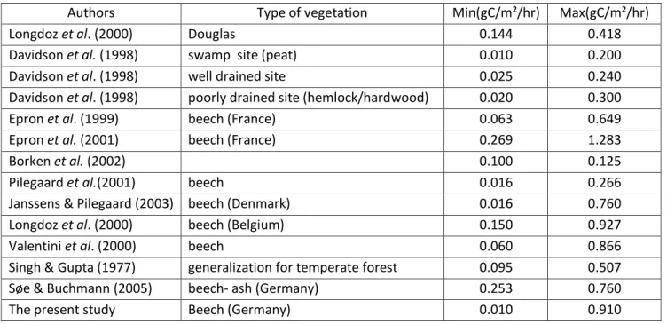
Authors Type of vegetation Min(gC/m²/hr) Max(gC/m²/hr)
Longdoz et al. (2000) Douglas 0.144 0.418
Davidson et al. (1998) swamp site (peat) 0.010 0.200
Davidson et al. (1998) well drained site 0.025 0.240
Davidson et al. (1998) poorly drained site (hemlock/hardwood) 0.020 0.300
Epron et al. (1999) beech (France) 0.063 0.649
Epron et al. (2001) beech (France) 0.269 1.283
Borken et al. (2002) 0.100 0.125
Pilegaard et al.(2001) beech 0.016 0.266
Janssens & Pilegaard (2003) beech (Denmark) 0.016 0.760
Longdoz et al. (2000) beech (Belgium) 0.150 0.927
Valentini et al. (2000) beech 0.060 0.866
Singh & Gupta (1977) generalization for temperate forest 0.095 0.507
Søe & Buchmann (2005) beech- ash (Germany) 0.253 0.760
The present study Beech (Germany) 0.010 0.910
Table 3: Soil CO2 efflux range from other studies
With values between 0.01 and 0.91 g.m-2.h-1, the soil CO2 efflux values we found are
equivalent to the one found in other studies (see Table 3), from 0.016 to 0.760 g.m-2.hr-1 in a Danish beech forest (Janssens & Pilegaard, 2003) but rather in the lower end when compared to studies from French beech forests (Epron et al. 2001: 0.269 to 1.283 g.m-2.h-1). The soil temperature at 10 cm explains 86% of the variation of soil CO2 fluxes of the site,
which is in the range of the results found by other studies based on exponential fit (around 80%; Davidson et al, 1998; Borken et al., 2002).
The predicted values are always above the measured one for the same temperature. A possible explanation is that our models are only based on soil temperature. Perrin et al. (2004) have shown that modeling only with temperature always overestimates the fluxes. Moreover the study site was a relatively wet site. Following the work of Perrin et al. (2004), above 0.27, the soil’s pores are saturated and therefore the flux of carbon can decrease. And in our site, the SWC was nearly always above that value. Refining our model with the SWC could help getting a better fit and a better correlation.
Role of the geophytes:
We found that the RSS of the models were better when the spots with and without geophytes were separated, that implies the impact of the factor ‘geophytes presence’ on the model. That was a first clue on the possible impact of the plants. Seasonal estimates of soil
18 CO2 fluxes were different between geophyte and non-geophyte spots, but these differences
were not significant. Maybe the latter, is due to lack of precision of the model. This could well be the case, because when using the measured values, a small but significant difference between geophyte spots and non-geophyte spots was found. The mean soil CO2 efflux is
slightly higher on geophyte spots than on non-geophyte spots.
General evidence regarding the influence of forest understory vegetation on soil properties and/or soil CO2 efflux is hard to find but differences between coniferous and broad-leaved
forests or between forest ecosystems and grasslands are known (Raich & Tufekcioglu, 2000). Some studies showed that the vegetation had an impact on the soil CO2 efflux by influencing
several soil characteristics (quality of litter, C:N ratio, nutrient level, …) (Vincent G., 2006; Longdoz et al. 2000 ; Fang et al., 1998 ). In our site, there weren’t any correlations between C:N ratio and soil CO2 efflux independent of geophyte presence. It seems that the geophyte
spots have a tendency to get a lower C and N content in the 0 to 10 cm soil layer but the difference to the non-geophytes spots was not significant.
Link between soil CO2 efflux and rFRB:
We found no correlation between soil CO2 efflux and rFRB in our sites, even if roots are in
general a major source of CO2 in the soil and the FRB is one of the major components of
belowground biomass (Tufekcioglu et al., 1999). Jurasinski et al., (2012) found a good relation between the FRB and the rFRB (R²=0,89) in the Hainich forest (Germany) at least for Ash roots. But they couldn’t find the same for beech fine roots. In the light of the fact that beech is the constituting species in our site it is understandable that we did not find a good correlation. Further, one has to keep in mind that the model was calibrated for an unmanaged old forest of central Germany and was just adapted to the Stuthof’ forest. Additionally we used the Jurasinski et al. (2012) beech model for all our species which might have introduced further bias.
Be it as it may, it is also worth to mention that rFRB may not be a good predictor for soil CO2
efflux in general: In a recent study, Zhu et al., (2009) found that the coarse root biomass was much more closely related to the soil CO2 efflux in mixed forests than FRB.
19
Conclusion
&
By defining the geophyte spots as the spots having geophytes and the non-geophytes spots as spots without geophytes, a positive impact of the presence of geophytes on soil CO2 efflux
has been shown. However, we didn’t find any significant differences between soil carbon content, soil nitrogen content and C:N ratio between geophyte and non-geophyte spots, and so no visible impact from the geophytes on soil parameters. This implies that only the presence of the plant alters the soil CO2 efflux. Still, it would be interesting to continue the
research on that topic by changing the definition of geophytes spots and using geophyte cover instead to define them. Further, enhancing the acquisition soil parameters by including pH, root biomass, microbial biomass and microbial activity would be useful as they are important . It could help assessing if there really aren’t any change in the soil where the geophytes grow, and so knowing precisely if and on which parameter the geophytes have an impact and use the result to improve the model.
The absence of correlation between rFRB and soil CO2 efflux could be overcome by
calibrating the model specifically with the site data and by developing better models for the other species. In its current form the results are not convincing and given the fact that no relation was found in Jurasinski et al. (2012) for other trees than Ash shows that this subject is still ongoing research and the model results are not satisfying yet.
It would be also interesting to include the factor ‘geophyte’ directly into the soil CO2
modeling, by looking more precisely on how it impacts the soil CO2 efflux. Thus, it should be
possible to integrate the different parameters that are influenced by geophyte presence in a model. This can only be fruitful if the definition of geophyte spots has been refined (see Appendix).
20
Bibliography
&
Ammer, Ch., S. Wagner. « An approach for modelling the mean fine-root biomass of Norway spruce stands ». Trees - Structure and Function 19, no. 2 (2005): 145-153.
Borken, Werner, Yi-Jun Xu, Eric A. Davidson, Friedrich Beese. „Site and Temporal Variation of Soil Respiration in European Beech, Norway Spruce, and Scots Pine Forests“. Global Change Biology 8, Nr. 12 (2002): 1205–1216.
Cox P. M., Betts R.A., Jones C.D., Spall S.A., Totterdell I.J. Acceleration of global warming due to carbon-cycle feedbacks in a coupled climate model. Nature 408, (2000): 184-187. Dafni, A., C. Dan, I., Noy-Meir. « Life-cycle variation in geophytes ». Annals of the Missouri
Botanical Garden (1981): 652.
Davidson EriC. A., Elizabeth Belk, Richard D. Boone. „Soil Water Content and Temperature as Independent or Confounded Factors Controlling Soil Respiration in a Temperate Mixed Hardwood Forest“. Global Change Biology 4, Nr. 2 (1998): 217–227.
Ellenberg H, Leuschner Ch. «Vegetation Mitteleuropas mit den Alpen». Ulmer Verlag, Stuttgart, (2010): 1334.
Epron, Daniel, L Farque, Eric Lucot, Pierre-Marie Badot. « Soil CO2 efflux in a beech forest: Dependence on soil temperature and soil water content ». Annals of Forest Science 56, no. 3 (1999): 221-226.
Epron, Daniel, Laetitia Farque, Eric Lucot, Pierre-Marie Badot. « Soil CO2 efflux in a beech forest: the contribution of root respiration ». Annals of Forest Science 56, no. 4 (1999): 7.
Epron, Daniel, Valerie Le Dantec, Eric Dufrene, Andre Granier. « Seasonal dynamics of soil carbon dioxide efflux and simulated rhizosphere respiration in a beech forest ».
Tree Physiology 21, no. 2-3 (2001): 145 -152.
Fang, C., John B. Moncrieff, Henry L. Gholz, Kenneth L. Clark. « Soil CO2 efflux and its spatial variation in a Florida slash pine plantation ». Plant and Soil 205, no. 2 (1998): 135-146.
Granier, A., E. Ceschia, C. Damesin, E. Dufrêne, D. Epron, P. Gross, S. Lebaube, et al. « The Carbon Balance of a Young Beech Forest ». Functional Ecology 14, no. 3 (2000): 312-325.
21 Hanson, P. J., Edwards, N. T., Garten, C. T., Andrews, J. A. « Separating root and soil microbial contributions to soil respiration: a review of methods and observations ».
Biogeochemistry 48, no. 1 (2000): 115–146.
Hermy, M., O. Honnay, L. Firbank, C. Grashof-Bokdam, J. E Lawesson. « An ecological comparison between ancient and other forest plant species of Europe, and the implications for forest conservation ». Biological conservation 91, no. 1 (1999): 9–22.
Herrmann, N., G. Weiss, W. Durka. « Biological flora of Central Europe: Muscari tenuiflorum Tausch ». Flora-Morphology, Distribution, Functional Ecology of Plants 201, no. 2 (2006): 81–101.
IPCC, Contribution of Working Groups I, II and III to the Fourth Assessment Report of the Intergovernmental Panel on Climate Change, Geneva, Switzerland. (2007): 104. Janssens, Ivan A., Kim Pilegaard. „Large Seasonal Changes in Q10 of Soil Respiration in a
Beech Forest“. Global Change Biology 9, Nr. 6 (2003): 911–918.
Jurasinski, G., Jordan A., Glatzel, S.« Mapping soil CO2 efflux in an old-growth forest using regression kriging with estimated fine root biomass as ancillary data ». Forest
ecology and management 263, no. 1 (2012): 101.
Lloyd J., Taylor J. A. „On the Temperature Dependence of Soil Respiration“. Functional Ecology 8, Nr. 3 (1994): 315–323.
Longdoz, B., M. Yernaux, M. Aubinet. « Soil CO2 Efflux Measurements in a Mixed Forest: Impact of Chamber Disturbances, Spatial Variability and Seasonal Evolution ».
Global Change Biology 6, no. 8 (2000): 907-917.
Morschhauser, T., K. Rudolf, Z. Botta-Dukát, B. Oborny. « Density-dependence in the establishment of juvenile< i> Allium ursinum</i> individuals in a monodominant stand of conspecific adults ». Acta Oecologica 35, no. 5 (2009): 621–629.
Perrin, Dominique, Éric Laitat, Michel Yernaux, Marc Aubinet. « Modélisation de la réponse des flux de respiration d’un sol forestier selon les principales variables climatiques ». Biotechnoogy, Agronomy, Society and Environment 8, no. 1 (2004): 15-26.
Pilegaard, K, P Hummelshøj, N.O Jensen, Z Chen. „Two years of continuous CO2 eddy-flux measurements over a Danish beech forest“. Agricultural and Forest Meteorology 107, Nr. 1 (2001): 29–41.
Raich, J, W., Tufekciogul, A, „Vegetation and soil respiration: Correlations and controls“. Biogeochemistry 48, Nr. 1 (2000): 71–90.
22 Revelle, Roger, Hans E. Suess. « Carbon Dioxide Exchange Between Atmosphere and Ocean and the Question of an Increase of Atmospheric CO2 During the Past Decades ». Tellus 9, nᵒ. 1 (1957): 18–27.
Service de l’observation et des statistiques (2011). Chiffres clés du climat, France et Monde. Repères – Janvier 2011
Singh, J., S. Gupta. „Plant decomposition and soil respiration in terrestrial ecosystems“. The Botanical Review 43, Nr. 4 (1977): 449–528.
Søe, Astrid R. B., Nina Buchmann. „Spatial and Temporal Variations in Soil Respiration in Relation to Stand Structure and Soil Parameters in an Unmanaged Beech Forest“. Tree Physiology 25, Nr. 11 (Januar 11, 2005): 1427–1436.
Tufekcioglu, A., J. Raich, T. Isenhart, R. Schultz. „Fine Root Dynamics, Coarse Root Biomass, Root Distribution, and Soil Respiration in a Multispecies Riparian Buffer in Central Iowa, USA“. Agroforestry Systems 44, Nr. 2 (1998): 163–174.
Valentini, R., G. Matteucci, A. J. Dolman, E.-D. Schulze, C. Rebmann, E. J. Moors, A. Granier, et al. « Respiration as the Main Determinant of Carbon Balance in European Forests ». Nature 404, nᵒ. 6780 (avril 20, 2000): 861-865.
Vincent, G. « Etude de la variabilité spatiale et temporelle dela respiration de sols forestiers hydromorphes à ennoyage temporaire ». Science de la Vie, Université de Franche Comté, 2006. http://artur.univ-fcomte.fr/ST/BIOECO/these/vincent_gaelle.pdf. Zhu, Jiaojun, Qiaoling Yan, A’nan Fan, Kai Yang, Zhibin Hu. „The role of environmental, root,
and microbial biomass characteristics in soil respiration in temperate secondary forests of Northeast China“. Trees - Structure and Function 23, Nr. 1 (2009): 189– 196.
Appendix:
Toward a definition of Geophytes spots&
Several definitions are possible to separate geophyte spots from non-geophyte spots. The one used throughout this work was to take the presence/absence of geophytes within the soil CO2 efflux measurement collars. After analyzing the results of the vegetation survey we
noticed that this definition might better be modified to one that uses the geophyte cover within the surroundings of the collar instead (see Table 4). Considering the percentage of cover of geophytes, the results differ considerably under different geophyte spot definitions (cover values ranging from above 30 to above 10%, see Figure 11) Using the cover separation method, for any percentage used, the non-geophyte spots have always a higher soil CO2 efflux than the geophyte spot. This contradicts the result found using the 1st
definition.
One reason might be that the vegetation survey has been made quite late during the season, so the results can be unreliable because some of the plants may already been dead and decayed. The first definition based on presence or absence of geophytes in the collars (decided throughout the measurement campaign) has been used for modeling and further analysis.
Figure 11: Difference between geophyte and non-geophyte spot according to the different definitions showed in Table 4.
0 Ta b le 4: D iff er ent de fini tion s f or di vi di n g the s pot be tw ee n ge oph yt es or non -ge oph yt es . C ol um n p3 0 to p1 0 re pre se nt the c ol la r w he re th e ge oph yt e s c ove r mor e t h an 30 to 10 pe rc en t of the s oi l r es pe ct ive ly, in the c ol um n pr es ence a ge oph yt e s pot is a c ol la r w h er e ge oph yt es gro w ins ide .
Transect Collars p30 p25 p20 p15 p10 presence Transect Collars p30 p25 p20 p15 p10 presence
1 0 0 0 0 0 0 31 1 1 1 1 1 1 2 0 0 0 0 0 1 32 0 0 0 1 1 0 3 0 0 0 0 0 1 33 0 0 0 0 1 1 4 0 0 0 0 0 1 34 1 1 1 1 1 0 5 0 0 0 0 0 1 35 0 0 0 0 0 0 6 1 1 1 1 1 1 36 0 1 1 1 1 1 7 1 1 1 1 1 1 37 1 1 1 1 1 0 8 1 1 1 1 1 1 38 0 0 0 0 0 1 9 0 0 0 1 1 1 39 0 0 0 0 1 0 10 0 0 0 0 1 1 40 0 0 0 0 1 0 11 0 0 0 0 1 0 41 0 0 0 1 1 1 12 0 1 1 1 1 1 42 0 0 1 1 1 1 13 0 0 0 0 0 1 43 0 0 0 0 0 0 14 0 0 0 1 1 1 44 1 1 1 1 1 0 15 0 0 1 1 1 0 45 0 0 0 0 0 0 16 0 0 0 0 0 1 46 0 0 0 1 1 1 17 0 0 0 0 0 1 47 0 0 0 0 0 1 18 0 0 1 1 1 1 48 0 0 0 0 0 1 19 1 1 1 1 1 0 49 0 0 1 1 1 0 20 1 1 1 1 1 1 50 0 0 1 1 1 0 21 0 0 0 1 1 0 51 0 1 1 1 1 1 22 0 0 0 0 0 0 52 0 1 1 1 1 0 23 0 0 0 1 1 1 53 0 0 0 0 1 1 24 0 0 0 0 0 0 54 1 1 1 1 1 1 25 0 0 0 0 0 1 55 1 1 1 1 1 0 26 1 1 1 1 1 1 56 0 0 0 0 0 0 27 0 0 1 1 1 0 57 1 1 1 1 1 1 28 1 1 1 1 1 1 58 1 1 1 1 1 0 29 1 1 1 1 1 1 59 0 0 0 0 0 1 30 1 1 1 1 1 0 60 0 0 1 1 1 1 1 2 3 4 5 6 7 8 9 10 11 12
Abstract
To define a forest as carbon sink or source the most important parameter is the soil carbon dioxide efflux (CO2). Several studies have been made to assess more precisely the involved factors. The
influence of soil temperature and humidity on soil CO2 efflux has since long been known and both
parameters are often included in current models. But there is still some variability that is more difficult to explain. Numerous factors, that have an effect on soil parameters, can impact the soil CO2 efflux. Recent studies showed that the fine root biomass (FRB) of trees had an influence on this
efflux. These studies have led to modeling of FRB for different tree species and their use in respiration models with more or less success.
A reason given to explain the lack of correlation between the modeled FRB (rFRB) was that the activity of spring geophytes could have an impact on the soil properties. Here, I show that the soil CO2 efflux of geophyte spots (~0.29 gC.m-2.hr-1) was significantly higher than that of non-geophyte
spots (~ 0.27 gC.m-2.hr-1). However, no impact of the presence of geophytes was found on soil carbon (C), nitrogen (N) content, or C:N.
Résumé
L’efflux de dioxyde de carbone (CO2) du sol est le paramètre qui peut avoir le plus d’impact sur la
détermination du rôle de puits ou de source de carbone d’une forêt. De nombreuses études ont été réalisées pour déterminer plus précisément les facteurs pouvant le faire varier. Si l’influence de la température ou encore de l’humidité du sol a été depuis longtemps mise en évidence et est bien prise en compte dans les modèles, il reste toujours une certaine variabilité qui est plus complexe à expliquer. En effet, de nombreux facteurs peuvent impacter cet efflux, notamment des facteurs ayant un impact sur les propriétés du sol. De récentes études ont montrés par exemple que la biomasse racinaire (FRB) des arbres avait une influence sur cet efflux de CO2. Ces études ont ensuite
aboutis sur des modèles de FRB pour les différentes espèces d’arbres et leur utilisation dans les modèles de respiration. Une raison avancée pour l’absence de corrélation entre la FRB modélisée et le flux de CO2 du sol est que l’activité des géophytes au printemps peut impacter certaines
propriétés du sol. Il a ici été mis en évidence que des points de mesures d’efflux du sol contenant des géophytes avait un efflux de CO2 (~0.29 gC.m-2.hr-1) légèrement (mais significativement) plus
important que ceux n’en ayant pas (~0.27 gC.m-2.hr-1). Aucun impact sur le contenu en carbone (C) ou en azote (N) du sol ainsi que sur le rapport C/N n’a pu être mis en évidence.