HAL Id: tel-00370418
https://tel.archives-ouvertes.fr/tel-00370418
Submitted on 24 Mar 2009
HAL is a multi-disciplinary open access
archive for the deposit and dissemination of sci-entific research documents, whether they are pub-lished or not. The documents may come from teaching and research institutions in France or abroad, or from public or private research centers.
L’archive ouverte pluridisciplinaire HAL, est destinée au dépôt et à la diffusion de documents scientifiques de niveau recherche, publiés ou non, émanant des établissements d’enseignement et de recherche français ou étrangers, des laboratoires publics ou privés.
Olivier P. Faugeras
To cite this version:
Olivier P. Faugeras. Contributions à la prévision statistique. Mathématiques [math]. Université Pierre et Marie Curie - Paris VI, 2008. Français. �tel-00370418�
TH`
ESE DE DOCTORAT
DE L’UNIVERSIT´
E PIERRE ET MARIE CURIE
Ecole doctorale de Sciences math´ematiques de Paris-Centre (ED 386)
Sp´ecialit´e : Statistique Math´ematique
Pr´esent´ee par: M. Olivier Paul FAUGERAS
Pour obtenir le grade de
DOCTEUR DE L’UNIVERSIT´
E PIERRE ET MARIE CURIE
Sujet de la th`ese : Contributions `a la pr´evision statistique
Soutenue le 28 Novembre 2008, devant le jury compos´e de :
• M. Marc HALLIN, Pr´esident du jury
• M. Denis BOSQ, Directeur de th`ese
• M. Christian GENEST, Rapporteur
• Mme. Hannelore LIERO, Rapporteur
• M. Patrice BERTAIL, Examinateur
Remerciements
Au moment de mettre un point final `a cette th`ese, je tiens `a remercier toutes les personnes qui m’ont aid´e `a mener `a bien ce travail, et en particulier les membres de mon jury. En premier lieu, je voudrais remercier chaleureusement M. Denis Bosq, Professeur Em´erite `a l’Universit´e Pierre et Marie Curie, d’avoir ´et´e mon directeur de th`ese. Merci `a M. Marc Hallin, Professeur `a l’Universit´e Libre de Bruxelles, qui me fait l’honneur de pr´esider le jury de cette th`ese. Merci `a M. Christian Genest, Professeur `a l’Universit´e Laval `a Qu´ebec, et `a Mme Hannelore Liero, Professeur `a l’universit´e de Postdam, d’avoir accept´e de juger ce travail et d’en avoir ´et´e les rapporteurs. Leurs remarques et suggestions ont ´et´es pr´ecieuses pour l’am´elioration de la qualit´e de ce manuscrit. Je suis par ailleurs extrˆemement reconnaissant `a M. Christian Genest de l’accueil qu’il m’a r´eserv´e au congr`es de la SSC-SFdS `a Ottawa et des ´echanges que nous avons pu avoir. Merci `a MM. les Professeurs Patrice Bertail, de l’Universit´e Paris X, et Michel Broniatowski, de l’Universit´e Pierre et Marie Curie, de me faire aussi l’honneur d’avoir accept´e de participer `a ce jury en tant qu’examinateurs.
Je veux aussi remercier M. Paul Deheuvels, Professeur `a l’Universit´e Paris 6, de m’avoir accueilli dans son DEA, puis dans son laboratoire. Je voudrais remercier `a ce titre tous les membres du LSTA, ainsi que les personnes que j’ai eu la chance de rencontrer dans les laboratoires Lim& Bio de Paris 13 et Modal’X de Paris 10, Nanterre. Je tiens ainsi `a remercier plus particuli`erement MM. Emmanuel Guerre, de l’Universit´e Queen Mary de Londres, G´erard Biau et Philippe Saint-Pierre, de l’Universit´e Pierre et Marie Curie
pour leurs encouragements et leurs conseils d´ecisifs `a l’accomplissement de ce travail, MM. Francesco Russo et Alain Venot de l’Universit´e Paris 13 pour m’avoir accueilli `a Paris 13 et donn´e l’occasion de faire connaˆıtre mon travail, MM. Armelle Guillou de l’Universit´e de Strasbourg, Karine Tribouley de l’Universit´e Paris 10, Taoufik Bouezmarni de HEC Montr´eal, Alexandre Leblanc de l’Universit´e du Manitoba et Johan Segers de l’Universit´e Catholique de Louvain pour l’int´erˆet qu’ils ont manifest´e dans ma recherche, et bien d’autres qui ont grandement contribu´e `a la r´eussite de cette th`ese.
Merci aux jeunes docteurs, pass´es ou `a venir, notamment Fran¸cois-Xavier Lejeune, Lahcen Douge, Kaouthar El Fassi, Pierre Ribereau, Esterina Masiello, Clara Zelli, Gwla-dys Toulemonde, Olivier Bouaziz, Claire Coiffard, Rawane Samb entre autres, pour m’avoir soutenu au cours de ces ann´ees. Merci bien sˆur `a Anne Durrande, Louise Lamart et Pascal Epron pour leur d´evouement au labo et leur gentillesse. Merci enfin `a toutes celles et ceux qui m’ont accompagn´e pendant cette aventure et dont la place me manque ici pour les ´enum´erer tous.
A mon p`ere, Paul-Etienne Faugeras,
Docteur en Physique, ancien chercheur au CERN, 1938-2008.
Contents
Acknowledgements 2
General introduction 13 1 Some generalities on statistical prediction 23
1.1 Some elements of statistical prediction theory . . . 24
1.1.1 The general prediction model . . . 24
1.1.2 Decomposition of the prediction error . . . 25
1.1.3 Statistical prediction theory and statistical estimation theory . . . . 26
1.2 Asymptotic prediction for a stochastic process . . . 27
1.2.1 Formulation of the problem for a stochastic process . . . 27
1.2.2 Probabilistic and Statistical prediction . . . 28
1.2.3 Delineation of the asymptotic prediction problem . . . 30
1.2.4 Statistical Prediction is not regression estimation . . . 34
1.3 Asymptotic decoupling by temporal separation . . . 36
1.3.1 Time splitting . . . 36
1.3.2 Coupling in β-mixing . . . 37
1.3.3 Equivalent risks . . . 38
2 Asymptotic Statistical prediction for a parametric additive model 41 2.1 Introduction . . . 42
2.1.1 Motivation . . . 42
2.1.2 S´eparation temporelle . . . 43
2.1.3 Discussion sur le mod`ele . . . 44
2.2 Consistance du pr´edicteur statistique . . . 46
2.3 Exemple d’application . . . 50
2.4 Loi limite du pr´edicteur statistique . . . 52
2.4.1 Un lemme d’ind´ependance asymptotique . . . 52
2.4.2 Convergence en loi . . . 53
2.4.3 Discussion . . . 57
2.4.4 Cas de la m´emoire fixe . . . 57
2.4.5 Application `a la pr´evision d’un AR(l) . . . 58
3 A quantile copula approach to conditional density estimation 61 3.1 Introduction . . . 62
3.1.1 Motivation . . . 62
3.1.2 Estimation by kernel density smoothing . . . 62
3.1.3 Estimation by regression techniques . . . 63
3.1.4 A product shaped estimator . . . 65
3.2 Presentation of the estimator . . . 65
3.2.1 The quantile transform . . . 65
3.2.2 The copula representation . . . 67
3.2.3 Construction of the estimator . . . 68
3.3 Pointwise Asymptotic results . . . 71
3.3.1 Notations and assumptions . . . 71
3.3.2 Heuristic . . . 72
3.3.3 Weak and strong consistency of the estimator . . . 72
Table of contents 9
3.3.5 Asymptotic Bias, Variance and Mean square error . . . 76
3.4 Intermediate and auxiliary results . . . 78
3.4.1 Approximation of the pseudo-variables F (Xi) by their estimates Fn(Xi) . . . 78
3.4.2 Convergence of the kernel density estimator ˆgn . . . 79
3.4.3 Convergence of cn(u, v) . . . 81
3.4.4 An approximation proposition of ˆcn(u, v) by cn(u, v) . . . 82
3.4.5 An approximation of ˆcn(Fn(x), Gn(y)) by ˆcn(F (x), G(y)) . . . 87
3.5 Uniform consistency results . . . 89
3.5.1 Uniform consistency of the conditional density estimator . . . 89
3.5.2 Uniform consistency of the kernel density estimators . . . 90
3.5.3 Two Uniform approximation propositions . . . 92
4 Discussions, implementation and comparisons 99 4.1 A discussion on the marginals and suggested modifications of the estimator 100 4.1.1 On the asymptotic efficiency of the empirical transformations . . . 100
4.1.2 On the connection with variable bandwidths density estimators . . 107
4.1.3 Estimator with parametric margins . . . 109
4.1.4 Further remarks . . . 110
4.2 Practical implementation of the estimator . . . 111
4.2.1 On the infinities at the corners and the approximate observations . 111 4.2.2 Boundary bias correction . . . 113
4.2.3 On bandwidth selection . . . 115
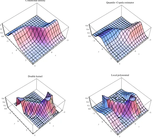
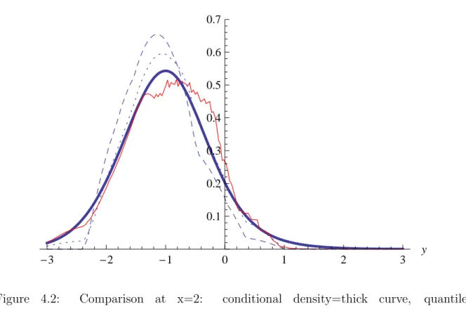
4.3 Simulations and comparison with other estimators . . . 119
4.3.1 Presentation of alternative estimators . . . 119
4.3.2 Asymptotic Bias and Variance comparison . . . 122
5 Application of conditional density estimation to prediction 129
5.1 Nonparametric statistical approaches to prediction . . . 130
5.1.1 Construction of Point predictors . . . 130
5.1.2 Predictive intervals and level sets . . . 131
5.2 Prediction by the conditional mode . . . 132
5.2.1 Asymptotic properties of the conditional mode predictor . . . 132
5.2.2 A remark on the practical implementation of the conditional mode predictor . . . 134
5.3 Prediction by intervals . . . 135
5.3.1 Determination of the level by a density quantile approach . . . 135
5.3.2 Calculation of predictive intervals . . . 136
5.4 Prediction by the conditional mean . . . 137
5.4.1 Consistency of the conditional mean predictor in the bounded case . 137 5.4.2 On the implementation of the conditional mean predictor . . . 138
5.4.3 On the asymptotic equivalence with Stute’s smooth k-Nearest Neigh-bour regression estimator . . . 139
6 Perspectives and possible applications 147 6.1 Variants and mathematical refinements of the conditional density estimator 148 6.2 Extensions of the proposed estimator . . . 150
6.2.1 Extension to the dependent case . . . 150
6.2.2 Extension to the multivariate case . . . 150
6.3 Estimation of the conditional cumulative distribution function . . . 152
6.3.1 On two possible approaches . . . 152
6.3.2 Application to point and interval prediction . . . 153
6.4 Some possible practical applications . . . 153
Table of contents 11 6.4.2 Estimation of conditional density for rare events . . . 154
Introduction et R´
esum´
e
Les Sciences naturelles et physiques s’attachent traditionnellement `a la compr´ehension du ph´enom`ene sous-jacent aux observations, par la cr´eation d’un mod`ele, dont la validit´e et la pertinence peut ˆetre remise en cause au cours d’une exp´erience. C’est par ce travail dialectique entre th´eorisation et exp´erimentation, que la connaissance scientifique pro-gresse. Pour citer H. Poincar´e dans La Science et l’hypoth`ese, mentionnons que si la science se construit `a partir de faits tir´es de l’exp´erience, “une accumulation de faits n’est pas plus une science qu’un tas de pierres n’est une maison.” Aussi, dans l’´elaboration de sa th´eorie, le scientifique doit soumettre constamment ses hypoth`eses `a la v´erification par l’exp´erience. Et pour accomplir ce travail de validation, “avant tout, le savant doit pr´evoir.”
C’est dire, outre son int´erˆet ´eminemment pratique, l’importance du probl`eme de la pr´evision, notamment pour fonder l’utilisation de la Statistique `a des fins scientifiques. Bien ´evidemment, le propos de cette th`ese est bien plus modeste en regard de ces en-jeux ´epist´emologiques. Le pr´esent travail traite de la Pr´evision Statistique. Il aborde ce probl`eme sous deux points de vue, param´etrique et non param´etrique, qui correspondent aux deux parties de cette th`ese.
En effet, la plupart des ph´enom`enes physiques dans la Nature ont un ´el´ement al´eatoire dans leur structure, qui fait que les grandeurs sont variables et ne peuvent ˆetre pr´evues avec certitude. Il est alors naturel d’adopter une approche Statistique. Un mod`ele proba-biliste est alors suppos´e d´ecrire le comportement du ph´enom`ene, qui ´evolue selon une loi
de probabilit´e.
• Dans la premi`ere partie de ce m´emoire, le mod`ele probabiliste est un processus stochastique, et l’on observe une s´erie temporelle, c’est-`a-dire une collection d’obser-vations effectu´ees s´equentiellement dans le temps, par exemple x1, . . . , xT. Des
exemples de s´eries temporelles abondent dans de nombreux domaines, notamment en ´economie, ing´enierie: elles peuvent correspondre `a des temp´eratures moyennes journali`eres, `a des cours de Bourse, etc... On cherche alors `a pr´edire une valeur future xT +h connaissant le pass´e x1, . . . , xT. La difficult´e du sujet a donn´e lieu `a de
multiples fa¸cons d’aborder ce probl`eme, voir par exemple Chatfield [34]. On suppose ici que l’on est dans un cadre param´etrique: les observations (xt) sont la r´ealisation
d’un processus stochastique (Xt) dont la loi est index´ee par un param`etre θ inconnu.
Une approche de type “plug-in” est alors d´evelopp´ee dans les chapitres 1 et 2. • Dans la seconde partie de ce m´emoire, l’approche abord´ee est quelque peu diff´erente.
Le mod`ele probabiliste est non-param´etrique, et on observe un ´echantillon de n couples de variables al´eatoires (Xi, Yi), i = 1, . . . , n, ind´ependants, identiquement
distribu´es. On cherche alors `a pr´edire, au sens d’expliquer, la variable Y par la vari-able pr´edictive X. L’int´erˆet se porte alors sur l’estimation de param`etres de position conditionnels, construits `a partir d’un estimateur de la densit´e conditionnelle. A cet effet, on propose et on ´etudie un nouvel estimateur de la densit´e conditionnelle (chapitres 3 `a 5).
Pr´
evision statistique param´
etrique des processus
(chapitres 1 et 2)
Dans le chapitre 1, nous donnons dans un premier temps quelques ´el´ements de la th´eorie g´en´erale de la pr´evision statistique param´etrique, telle qu’elle est d´evelopp´ee par Bosq
Introduction et R´esum´e 15 dans [24], chapitre 1. Nous particularisons ensuite le cadre de cette th´eorie `a la pr´evision statistique d’un processus stochastique. A cet effet, nous nous effor¸cons de clarifier ce probl`eme et de le distinguer des probl`emes li´es que sont ceux de la pr´evision probabiliste et de l’estimation de la r´egression. Une telle approche am`ene naturellement `a adopter un point de vue asymptotique, qui consiste, `a partir d’un estimateur ˆθT du param`etre
inconnu θ qui gouverne la loi du processus, `a construire un pr´edicteur de type “plug-in” , de la fonction de r´egression rθ(.). On obtient alors le pr´edicteur statistique
ˆ
XT +h := rθˆT(X1, . . . , XT).
Cependant, le fait que les mˆemes donn´ees servent `a la fois pour l’estimation du param`etre et pour le calcul du pr´edicteur rend cette approche difficile. A cet effet, nous pr´esentons un moyen de pallier `a cette difficult´e en d´ecouplant ces deux probl`emes de fa¸con asymptotique dans le cadre de processus m´elangeants. Plus pr´ecis´ement, nous mettons en oeuvre un proc´ed´e de s´eparation temporelle des donn´ees et montrons comment l’erreur de pr´evision peut ˆetre approch´ee asymptotiquement par une erreur quadratique int´egr´ee.
Dans le chapitre 2, nous mettons en oeuvre le proc´ed´e annonc´e sur une classe g´en´erale de processus qui suivent un mod`ele additif approximativement markovien. Plus pr´ecis´ement, on se place donc dans le cadre suivant o`u la fonction de r´egression rθ(.)
d´epend approximativement des kT derni`eres valeurs (XT −i, i = 1,· · · , kT) avec kT ≤ T ,
kT → ∞, c’est-`a-dire, XT +1∗ := Eθ£XT +1 ¯ ¯X−∞T ¤ := kT X i=0 ri(XT −i, θ) + ηkT(X, θ),
o`u chaque fonction ri repr´esente la contribution (additive) de la XT −i valeur, et o`u
ηkT(X, θ) est une fonction de carr´e int´egrable asymptotiquement n´egligeable dans un sens
`a pr´eciser. Ce mod`ele, qui est une extension d’un mod`ele ´etudi´e par Bosq [23], est suff-isamment large pour ˆetre applicable `a un certain nombre de cas particuliers, comme le mod`ele autor´egressif AR. En estimant θ par ˆθφ(T )sur l’intervalle [0, ϕ(T )] avec ϕ(T )→ ∞,
on construit alors le pr´edicteur statistique ˆ
Xt+1 = rθˆϕ(T )(XT −kT T).
Sous des conditions de m´elangeance et de r´egularit´e, on peut s´eparer le probl`eme d’estimation de θ sur [0, ϕ(T )] du probl`eme probabiliste sur la “m´emoire” du processus entre [T − kT, T ]. En effet, nous obtenons la consistance asymptotique dans le th´eor`eme
suivant,
Th´eor`eme 2.5 Si les hypoth`eses H0,H1,H2 sont v´erifi´ees, alors
lim sup
T →∞
Eθ( ˆXT +1− XT +1∗ )2 = 0
et la loi limite du pr´edicteur statistique, dans le th´eor`eme suivant. Th´eor`eme 2.10 Si les hypoth`eses H′
0,H′1,H′2 sont v´erifi´ees, alors
pϕ(T )( ˆXT +1− XT +1∗ ) d
❀< U, V >
o`u U et V sont deux variables ind´ependantes, U de loi N (0, σ2(θ)) et V la loi limite de +∞
P
i=0
∂θri(XT −i; θ).
Ces r´esultats sont ensuite appliqu´es sur des exemples.
Estimation non-param´
etrique de la densit´
e
condition-nelle et application `
a la pr´
ediction (chapitres 3 `
a 6)
Dans la premi`ere partie de cette th`ese, nous avons cherch´e comment d´ecoupler le probl`eme d’estimation et le probl`eme de pr´evision pure dans le probl`eme mixte de la pr´evision statistique. Par suite, dans la pr´evision de Y par X, ceci nous a amen´e `a nous int´eresser `a ´etudier la structure de d´ependance entre X et Y . Suites `a des consid´erations de sym´etrie, entendue au sens d’invariance, ces investigations se sont concr´etis´ees dans la proposition d’un nouvel estimateur de la densit´e conditionnelle.
Introduction et R´esum´e 17 Plus pr´ecis´ement, dans le chapitre 3, on se donne un ´echantillon de n couples de variables al´eatoires (Xi, Yi) ind´ependants, identiquement distribu´es et `a valeurs dans R×
R, et on cherche `a construire un estimateur non param´etrique de la densit´e conditionnelle f (y|x) de Y sachant que X = x. Une premi`ere approche, exploit´ee dans la litt´erature notamment par Rosenblatt [114], Bosq [20] et Roussas [115], consiste `a estimer les densit´es fXY de (X, Y ) et f de X par des estimateurs non param´etriques, notamment de type
Parzen [102] Rosenblatt [113], pour former un estimateur de forme quotient, `a partir de la d´efinition de la densit´e conditionnelle, comme
f (y|x) = fXY(x, y) f (x) .
Une seconde approche consiste `a transformer les donn´ees Yi en pseudo-donn´ees,
Yi′ := Kh(Yi− y) := 1 hK µ Yi− y h 
o`u K est un noyau de Parzen-Rosenblatt, et exploiter le fait que, par un th´eor`eme de type Bochner,
E (Y′|X = x) ≈ f(y|x), h → 0, pour effectuer la r´egression des pseudo-donn´ees Y′
i sur les Xi par des techniques
non-param´etriques telles que Nadaraya-Watson [99, 144], polynˆomes locaux, projections, etc.... L’approche que nous proposons consiste en quelque sorte `a combiner des ´el´ements de ces deux approches: en transformant les donn´ees en X et Y par leurs fonctions de r´epartition marginales respectives F et G, l’expression de la densit´e conditionnelle s’´ecrit sous la forme du produit suivant
f (y|x) = g(y)c(F (x), G(y))
o`u g est la densit´e de Y et c est la densit´e de copule, i.e. la densit´e jointe du couple de variable transform´ees (U, V ) := (F (X), G(Y )). Cette notion de copule, introduite par Sklar [122] au travers du th´eor`eme qui porte maintenant son nom, permet de s´eparer l’al´ea qui d´epend uniquement des marges du vecteur (X, Y ), de l’al´ea qui d´epend uniquement
de la structure de d´ependance entre X et Y . L’estimateur est alors construit `a partir des fonctions de r´epartition empirique et d’estimateurs `a noyau des densit´es, et s’´ecrit sous la forme suivante, ˆ fn(y|x) := " 1 nhn n X i=1 K0µ y − Yi hn ¶# . " 1 na2 n n X i=1 K1 µ Fn(x)− Fn(Xi) an ¶ K2 µ Gn(y)− Gn(Yi) an ¶¸ :=ˆgn(y)ˆcn(Fn(x), Gn(y)).
Nous ´etudions ses propri´et´es asymptotiques et obtenons, `a partir des r´esultats classiques de convergence des estimateurs `a noyau de la densit´e et sous les conditions usuelles de r´egularit´e sur les densit´es et les noyaux, les r´esultats suivants:
• Consistance ponctuelle en probabilit´e,
Th´eor`eme 3.5 Sous les conditions de r´egularit´e sur les densit´es et les noyaux, si hn et an tendent vers z´ero quand n → ∞ de fa¸con que nhn → ∞, na4n → ∞,
√ ln ln n na3 n → 0, alors ˆ fn(y|x) = f(y|x) + OP Ã 1 √ nhn + h2n+ a2n+ 1 pna2 n + 1 na4 n + √ ln ln n na3 n ! . Un choix de fenˆetres satisfaisant an ≃ n−1/6 et hn ≃ n−1/5 donne les vitesses de
convergences optimales pour les r´egularit´es consid´er´ees, ici n−1/3.
• Consistance ponctuelle presque sˆure,
Th´eor`eme 3.7 Sous les conditions de r´egularit´e sur les densit´es et les noyaux, si hn→ 0 et an→ 0 tels que ln ln nnhn → ∞, (ln n) 1/2(ln ln n)1/2 na3 n → 0, ln ln n na4 n → 0, alors ˆ fn(y|x) = f(y|x) + Oa.s. Ã h2n+r ln ln n nhn + a2n+ s ln ln n na2 n + ln ln n na4 n + (ln n) 1/2(ln ln n)1/2 na3 n ! .
Introduction et R´esum´e 19 Un choix de fenˆetres satisfaisant an ≃
¡ln ln n
n
¢1/6
et hn ≃ ((ln ln n/n))1/5 donne les
vitesses de convergences optimales pour les r´egularit´es consid´er´ees, ici (ln ln n/n)1/3.
• Convergence en loi,
Th´eor`eme 3.9 Sous les conditions de r´egularit´e sur les densit´es et les noyaux, si hn→ 0, an→ 0, tels que nhn → ∞, √ ln ln n na3 n → 0, na 4 n→ ∞, na6n→ 0, alors pna2 n³ ˆfn(y|x) − f(y|x) ´ d ❀N ¡0, g(y)f(y|x)||K||22¢ .
Ces r´esultats sont ensuite ´etendus sur des compacts de R, dans les th´eor`emes suivants: • consistance uniforme en y sur un compact en probabilit´e,
Th´eor`eme 3.18 Sous les conditions de r´egularit´e sur les densit´es et les noyaux, si hn ≃ (ln n/n)1/5 et an ≃ (ln n/n)1/6, alors, pour x appartenant `a l’int´erieur du
support de f et un intervalle [a, b] inclus dans l’int´erieur du support de g, sup y∈[a,b]| ˆ fn(y|x) − f(y|x)| = Op à µ ln n n ¶1/3! .
• consistance uniforme en y sur un compact presque sˆurement,
Th´eor`eme 3.18 Sous les conditions de r´egularit´e sur les densit´es et les noyaux, si hn ≃ (ln n/n)1/5 et an ≃ (ln n/n)1/6, alors, pour x appartenant `a l’int´erieur du
support de f et un intervalle [a, b] inclus dans l’int´erieur du support de g, sup y∈[a,b] ¯ ¯ ¯fˆn(y|x) − f(y|x) ¯ ¯ ¯ = Oa.s. Ã µ ln n n ¶1/3! .
De mˆeme que pour le cas ponctuel, le choix de fenˆetres pr´ec´edent donne une vitesse de convergence uniforme optimale pour les r´egularit´es consid´er´ees.
Dans le chapitre 4, les propri´et´es asymptotiques th´eoriques obtenues dans le chapitre pr´ec´edent sont compl´et´ees par des discussions dans plusieurs directions. Dans un premier temps, nous nous int´eressons `a l’efficacit´e des transformations empiriques des donn´ees par Fn et Gn. En nous appuyant notamment sur les travaux de Reiss [109] et la notion de
d´eficience introduite par Hodges et Lehmann [75], nous sugg´erons une modification de notre estimateur initial, o`u les fonctions de r´epartitions empiriques sont remplac´ees par des estimateurs liss´es ˆF , ˆG, `a noyau. De fa¸con similaire, lorsque le support des densit´es marginales est born´e, nous sugg´erons d’utiliser les estimateurs bas´es sur les polynˆomes de Bernstein introduits par Vitale [139]. Nous en profitons alors pour ´etablir une con-nection heuristique avec les estimateurs de la densit´e `a fenˆetre locale. La consistance de ces estimateurs modifi´es est montr´ee dans le corollaire 4.3. Enfin, nous pr´esentons une extension de l’estimateur dans un cadre semi-param´etrique, lorsque de l’information suppl´ementaire concernant la distribution de la variable explicative X peut-ˆetre incorpor´ee dans un mod`ele param´etrique (proposition 4.5). Dans un deuxi`eme temps, nous nous int´eressons `a l’implantation num´erique de l’estimateur propos´e. D’autres consid´erations sur la transformation des donn´ees nous am`enent `a recommander aussi l’utilisation d’autres estimateurs que les fonctions de r´epartition empirique. Nous recensons ensuite quelques techniques de r´eduction du biais de l’estimation de la densit´e de copule, notamment l’utilisation des noyaux Beta propos´es par Chen [35], ceci afin d’am´eliorer sensiblement les performances `a ´echantillon fini de l’estimateur. Enfin, nous esquissons une strat´egie de s´election des fenˆetres. Dans un troisi`eme temps, nous effectuons une br`eve simula-tion num´erique afin de comparer en pratique notre estimateur `a ses concurrents. Apr`es une comparaison th´eorique des biais et variances asymptotiques o`u nous montrons que notre estimateur a une variance plus petite d`es que le produit des densit´es marginales est inf´erieur `a l’unit´e, nous mettons en ´evidence sur un mod`ele la diff´erence de comportement li´ee `a la structure produit de notre estimateur face aux estimateurs alternatifs bas´es sur des structures de quotients. Plus pr´ecis´ement, les r´esultats num´eriques semblent montrer
Introduction et R´esum´e 21 un comportement prometteur de l’estimateur lorsque l’on s’int´eresse `a l’estimation de la densit´e conditionnelle pour de grandes valeurs de x, i.e. dans un domaine o`u l’on dispose de peu de donn´ees Xi, ce qui pourrait s’av´erer potentiellement int´eressant pour l’inf´erence
d’´ev´enements extrˆemes.
Dans le chapitre 5, nous montrons comment utiliser l’estimation de la densit´e con-ditionnelle comme une premi`ere ´etape pour construire des pr´edicteurs. On s’int´eresse notamment aux pr´edicteurs ponctuels que sont le mode et la moyenne conditionnelle, et aux intervalles de pr´evision couvrant une probabilit´e α donn´ee, comme les r´egions de plus grande densit´e, i.e. l’ensemble des valeurs de y telles que la densit´e conditionnellle d´epasse un seuil fα. En particulier, en ce qui concerne le mode conditionnel, nous montrons, `a
partir des r´esultats de convergence uniforme de la densit´e du chapitre 3, sa consistance dans la proposition suivante,
Proposition 5.2 Sous des hypoth`eses ad´equates, l’estimateur du mode conditionnel ˆ
θ(x) = arg supy∈S′fˆn(y|x) converge presque sˆurement vers le mode conditionnel θ(x) =
arg supy∈S′f (y|x).
et nous donnons quelques remarques sur son impl´ementation pratique. De fa¸con similaire, nous ´etablissons la convergence de l’intervalle de pr´evision [ˆyα, ˆyα] empirique, obtenu `a
partir de l’estimateur de la densit´e conditionnelle, vers l’intervalle de pr´evision th´eorique [yα, yα] dans la proposition suivante,
Proposition 5.4 Si le seuil empirique ˆfα converge p.s. vers le seuil th´eorique fα, alors
ˆ yα
a.s
→ yα et ˆyα a.s→ yα,
et indiquons aussi des m´ethodes pour sa d´etermination pratique. Enfin, nous nous int´eressons `a la moyenne conditionnelle, i.e. la fonction de r´egression, et ´etablissons un r´esultat de consistance dans le cas simple o`u le support de Y est born´ee (Proposition 5.5) ainsi qu’une connection asymptotique heuristique dans le lemme 5.7 avec l’estimateur des plus proches voisins en rangs de Yang [145] et Stute [128] similaire `a celle qui existe entre l’estimateur de la densit´e conditionnelle `a double noyau de Rosenblatt et Roussas
[114, 115] et l’estimateur de la r´egression de Nadaraya et Watson [99, 144].
En conclusion de cette partie, nous dressons bri`evement dans le chapitre 6 des per-spectives de recherche et d’applications possibles de cet estimateur, notamment pour l’inf´erence et l’estimation d’´ev`enements rares ou extrˆemes.
Chapter 1
Some generalities on statistical
prediction
Abstract : This chapter is of introductory nature. Its aim is to introduce the subject of statistical prediction by formulating the statistical prediction problem of predicting an unobserved value XT +h, with h > 0, of a stochastic process (Xt)t∈T given an observed
sample path (Xt)0≤t≤T, discussing its connections with other related topics, and preparing
the method of prediction developed in chapter 2. Starting from general considerations on statistical prediction in section 1.1, we progressively clarify this problem from the closely related ones of probabilistic prediction and regression estimation in section 1.2. In partic-ular, in the case where the law of the process is governed by an unknown parameter θ, we show that solving the problem amounts to calculating a plugged version of the estimated conditional expectation. From a statistical standpoint, these two issues, estimating the parameter and calculating the conditional expectation, are coupled, making the study of the statistical predictor difficult. To that end, we propose in the mixing framework a data-splitting device to separate these two issues in section 1.3. More precisely, we show that an approximation of the prediction error is asymptotically close to the true prediction
error. A concrete application of this device to a class of processes is developed in chapter 2.
1.1
Some elements of statistical prediction theory
In this section, we give some elements of the general parametric statistical prediction theory, as developed by Bosq in [24], chapter 1.
1.1.1
The general prediction model
Let (Ω,A, P ) a probability space and note X and Y two sub-algebras of A, standing for the collection of observed and non-observed events, respectively. To be more specific, assume the probability law is indexed by a parameter θ ∈ Θ, where Θ is a parameter space, so that we are given the parametric statistical model (Ω,A, Pθ, θ ∈ Θ). Moreover,
assume that X = σ(X), where X stands for the collection of observed random variables and takes its values in a measurable space (X, X ).
In the prediction of a Y-measurable real-valued random variable Y by a X -measurable random variable X, one is interested in finding a function p, which be X -measurable, such that p(X) represents a good approximation of the unobserved Y . More generally, one can also consider the prediction of a given known function of X, Y and θ. To that purpose, define the predictand g(X, Y, θ)∈ ∩θ∈ΘL2(Pθ), where g is a known function, and
the predictor p(X) to be any measurable function of X, where p is known, assumed also to be such that p(X)∈ ∩θ∈ΘL2(Pθ).
The quality of this approximation is evaluated by the quadratic prediction error
Rθ(p, g) := Eθ(p(x)− g(X, Y, θ))2, θ∈ Θ. (1.1)
Such a criteria induces the following preference relation:
1.1 Some elements of statistical prediction theory 25 only if Rθ(p1, g)≤ Rθ(p2, g), θ∈ Θ. If so, one notes p1 ≺ p2.
The prediction problem of g(X, Y, θ) can be split into several cases, depending on the structure of the predictand considered:
• if g is a function of Y only, one has a pure prediction problem; • if g is a function of θ only, one has a pure estimation problem; • in any other case, one has a mixed problem.
1.1.2
Decomposition of the prediction error
The simple lemma below, which belongs to folklore, gives a fundamental decomposition of the quadratic prediction error, (see e.g. lemma 1.1 of [24]):
Lemma 1.2 The following decomposition of the Quadratic Prediction Error holds, Rθ(p, g) = Eθ[(g(X, Y, θ)− Eθ[g(X, Y, θ)|X])2] (1.2)
+ Eθ[(Eθ[g(X, Y, θ)|X] − p(X))2]
Rθ(p, g) := P P Eθ(g) + SP Eθ(p, g)
Hence, p1 ≺ p2 for predicting g if and only p1 ≺ p2 for predicting Eθ[g|X].
Proof It simply follows from the Pythagorean property of the conditional expectation. The consequences of this lemma are twofold:
• A lower bound on the prediction error is given by the Probabilistic Prediction Error P P Eθ(g) := Eθ[(g(X, Y, θ)− Eθ[g(X, Y, θ)|X])2], which is not controllable by the
Statistician. Therefore, the Statistician can only try to minimise the Statistical Prediction Error SP Eθ(p, g) := Eθ[(Eθ[g(X, Y, θ)|X] − p(X))2].
• For the case where g is a known function of Y only, i.e. when g(X, Y, θ) = g(Y ), predicting g(Y ) is therefore equivalent to predicting Eθ[g(Y )|X]. The latter being a
function of X and θ, one sees that, in general, a non degenerate prediction problem is mixed.
1.1.3
Statistical prediction theory and statistical estimation
theory
Parallelling the theory of parametric statistical estimation theory as exposed, e.g. in Lehmann and Casella [92], an analogue theory can be constructed as developed in Bosq and Blanke [24] and Bosq [22], which we briefly sketch below. In the context of pre-diction, the counterpart of sufficient statistics are prediction sufficient statistics, which add a conditional independence condition to the sufficiency one . Thanks to such predic-tion sufficient statistics, a Rao-Blackwell type theorem for predicpredic-tion can be formulated. Optimality can be investigated in a similar fashion to that of UMVU estimation. Ad-missibility considerations implies that the search for optimal predictors is restricted to the class of unbiased ones. The unique optimal unbiased predictor is then characterised by a Lehmann-Scheff´e theorem. Under regularity conditions, Cram´er-Rao bounds can be obtained. We refer the interested reader to the detailed exposition of Bosq and Blanke [24].
Remark 1.3 Other criteria than the quadratic prediction error can also be considered. In a decision theoretical framework `a la Wald [141], a risk is defined through the expectation of a positive loss function L by Eθ[L(p, g)]. Special interest lie in loss functions associated
with a location parameter µ = µθ. In the real valued case, for a random variable Z,
µ is defined as EθL(Z, µ) = mina∈REθL(Z, a). Since EθL(g, p) = Eθ[Eθ[L(g, p)|X]] is
minimum for pθ(X) = µθ(X), the following classical loss functions allow to define the
1.2 Asymptotic prediction for a stochastic process 27 • for the square loss L(u, v) = (u − v)2, µ
θ(X) is the conditional mean Eθ[g|X];
• for the absolute value loss L(u, v) = |u − v|, µθ(X) is the median of the conditional
distribution of g given X;
• for the 0 − 1 loss L(u, v) = 1|u−v|>ǫ for ǫ > 0, µθ(X) is the mode of the conditional
distribution of g given X;
The advantage of the square loss is that it simplifies the mathematical treatment of the problem as shown, e.g., in lemma 1.2 above. Other choices such are possible such as the 0− 1 loss, especially for random variables taking their values in a discrete set, or the absolute value loss or the Huber loss (See Huber [79]), often motivated by robustness considerations, which we will not pursue here. A different approach in a non parametric framework, by estimation of these conditional locations parameters is pursued in chapter 5.
1.2
Asymptotic prediction for a stochastic process
In this section, we particularise the above framework to the context of a time series, and intend to clarify it with the related problems of probabilistic prediction and regression estimation.
1.2.1
Formulation of the problem for a stochastic process
To that purpose, let (Xt)t∈T be a real-valued square integrable stochastic process defined
on a probability space (Ω,A, Pθ), with θ ∈ Θ. For T = Z, (Xt)t∈Z is a discrete time
stochastic process, and one observes the past X = (X1, . . . , XT) and intends to predict
the future Y = XT +h, where h ∈ N is the horizon. For T = R, (Xt)t∈R is a continuous
time stochastic process, and one observes X = (Xt, 0 ≤ t ≤ T ) and intends to predict
In various situations, no optimal predictor may exist (see e.g. lemma 1.2 of Bosq and Blanke [24]) or may be extremely difficult to compute (see subsections 1.2.2 below). As is the case for statistical estimation theory, we will show below that it is therefore natural to adopt an asymptotic point of view, with sample size tending to infinity. To that purpose, we index the data X from which a statistical predictor has to be built by time T . To prevent confusion, we rename the X vector as DT, i.e. we define the observed
past DT := (X1, . . . , XT) or DT := (Xt, 0 ≤ t ≤ T ) for discrete or continuous time,
respectively. The statistical predictor will be noted ˆXT +h and thus is a random variable
which is σ(DT) measurable, i.e. such as there exists a function p ∈ L2(P ) such that
ˆ
XT +h = p(DT). We are bound to make the following distinction in order to separate the
problems.
1.2.2
Probabilistic and Statistical prediction
Probabilistic Prediction
In the present context, lemma 1.2 writes
Eθ(XT +h− p(DT))2 = Eθ[XT +h− Eθ(XT +h|DT)]2 (1.3)
+ Eθ[Eθ(XT +h|DT)− p(DT)]2
and the theoretical answer to the minimisation problem of the statistical prediction error is given by the so-called Bayes or Probabilistic predictor, defined as
XT +h∗ := Eθ(XT +h|DT). (1.4)
From a probabilistic standpoint, i.e. assuming the knowledge of the parameter θ, the prediction problem thus reduces to the calculation of the conditional expectation 1.4.
1.2 Asymptotic prediction for a stochastic process 29 Examples of probabilistic prediction
Depending on the assumed model on the process, the calculation of the conditional expec-tation may be more or less difficult. This problem has been tackled by numerous people and a huge literature is devoted to the subject. We sketch below only a glimpse of the topic.
• Linear prediction Assume Xt is a Gaussian process in discrete time. Then, since
(XT +h, DT) is a Gaussian vector, the conditional expectation 1.4 reduces to a linear
function of the DT, and the search for the Bayes predictor reduces to the search for
the best linear predictor.
• Kolmogorov-Wiener theory For weakly stationary square integrable time series and predictors restricted to the class of linear predictors, a complete solution is provided by the work of Kolmogorov and Wiener, cf. e.g. [29].
• Filtering and Control for Diffusion processes For a diffusion process satisfying the stochastic differential equation,
dXt= a(Xt, t)dt + σ(Xt, t)dWt
where (Wt)t∈T is a Wiener process, and the functions a and b are assumed to be
known, the conditional expectation calculation was solved by Kallianpur and Zakai. We refer the reader to the vast literature (see e.g. [84] and the references therein) on the related problems of stochastic control and filtering of stochastic processes. • Markov If the process is assumed to be Markovian of order m, then the conditional
expectation Eθ(XT +h|DT) reduces to Eθ(XT +h|XT, . . . , XT −m+1).
Statistical prediction
However, from a statistical standpoint, the solution 1.4 is not satisfactory, since we as-sumed the knowledge of the underlying model of the process. Indeed, this probabilistic
predictor is not a genuine statistical predictor depending only on the data DT, since it is
also a function of the unknown parameter θ. As a consequence, it can not used by the statistician to make a practical prediction.
The mixed nature of the statistical prediction problem, as announced in section 1.1, clearly appears here. One both has
1. a purely statistical problem of estimation of the unknown law of the process built from the data DT,
2. a purely probabilistic problem of the calculation of the conditional expecta-tion Eθ(XT +h|DT) , i.e. of calculation of the regression function rθ(dT) :=
Eθ(XT +h|DT = dT).
As the unknown θ has to be estimated, it is therefore natural to adopt an asymptotic point of view. A possible solution to overcome this mixed difficulty may consist in
1. estimating θ by an estimator ˆθT from the data DT,
2. building a plug-in type statistical predictor from the regression function rθ(dT) :=
Eθ(XT +h|DT = dT), by
ˆ
XT +h := rθˆT(DT).
However, the fact that the same data DT is involved in both problems, renders the
asymp-totic behaviour of this statistical predictor difficult to study. Before presenting a partial remedy for this issue in section 1.3, we sketch below some clarifications between this prediction problem and related approaches.
1.2.3
Delineation of the asymptotic prediction problem
Note that in the remainder of this chapter, we temporally omit the parameter θ indexing the law of the process, in order to simplify notations.
1.2 Asymptotic prediction for a stochastic process 31 Taking into account asymptotics, there are several other distinctions we would like to clar-ify, which depend on the features the Statistician wants to incorporate in the formulation of his problem:
Probabilistic versus Empirical Error
The quadratic prediction error 1.1 writes here as
RT( ˆXT +h, XT +h) := E(XT +h− p(DT))2. (1.5)
Note that this risk, defined as an expected loss, although it gives the theoretical error, is not observable by the Statistician, since the distribution of the process is usually unknown. Consequently, the Statistician can also choose to measure the prediction error by an empirical criteria. To that end, the problem is cast in a sequential fashion. In the discrete time case and when the goal is to predict the next value (i.e. h = 1), at each time instant t = 1, 2, . . ., a sequence of predictors pt(Dt−1) is constructed, based on the
values of (X1, X2, . . . , Xt−1). After T time instants, the normalised cumulative empirical
prediction error of the strategy p consisting of the sequence of predictors {pt}, is
ReT(p, X) := 1 T T X t=1 (pt(Dt)− Xt)2 (1.6)
which is termed the Ces´aro loss by [66]. The connections between these probabilistic and empirical sequential errors 1.5 and 1.6 are investigated by Algoet [6, 7], Gy¨orfi et al. [66] chapter 27. See also the discussion below on the static and dynamic forecasting problem. This empirical measure of the error allows to reformulate the problem in a repeated game-theoretic framework, building on the pioneering work of Blackwell [19] on approachability theory, as exemplified by the recent monograph of Cesa-Bianchi and Lugosi [32] on the prediction of individual sequences. Since the error is now observable, it can be used as side information in order to find solutions of the minimizing of 1.6 in a recursive way. Such an approach, which has the advantage of not making assumptions on the underlying
process governing the time series, consists in combining several base predictors according to their past performances, mirroring the gradient optimisation algorithms of the dynamic programming paradigm (See Cesa-Bianchi and Lugosi [32] and the references therein). Assumptions on the process and the predictors
Parallelling the approach of statistical estimation where the Statistician can decide to restrict the search of estimators to the family of unbiased ones - which leads to the development of UMVU estimation, the Statistician may also decide to set limitations on the space of possible predictors. One can distinguish mainly between two kind of limitations,
• Shape constraints: the Statistician can make structural assumptions on the shape of the possible functions p, e.g. to be linear in the predictands, i.e. in the discrete time case, p(DT) = PTi=1aiXi, where ai ∈ R, i = 1, . . . , T .
• Memory size: instead of taking into account all of the possible past to make his prediction, he can decide to limit himself to finite memory predictors, i.e. functions of the m-proximity past, p(DT) = p(XT, XT −1. . . , XT −m+1) in the discrete time
case.
In a dual manner, the Statistician can make assumptions on the stochastic process gov-erning the observed time series. Among others, he can impose some structure such as a Gaussian or a Markov one. These limitations in the predictors space are strongly con-nected with the assumptions one is willing to make on the stochastic process. Gaussian and Markov hypothesis lead naturally to these limitations, as was mentioned in the ex-amples of subsection 1.2.2 above.
1.2 Asymptotic prediction for a stochastic process 33 Static versus Dynamic forecasting.
Taking into account asymptotics, there are two more distinctions to be made for the prediction of stationary ergodic processes, depending on the way one goes to infinity, as formulated by Cover [38].
• Dynamic forecasting: One fixes the beginning of the observed series, and search for a prediction of the process in the infinite future. In other words, DT = (X1, . . . , XT)
is the data, XT +1 is the value to be predicted, and one looks for a sequence of
predictors p = (pT), such that
lim
T →∞|pT(DT)− E[XT +1|DT]| = 0 a.s.
• Static forecasting: One fixes the time of prediction, and look back in the increasing past D′T = (X−T, . . . , X−1, X0) to make a prediction of X1. In other words, one look
for a predictor p such that lim
T →∞p(D ′
T) = E[X1|X0, X−1, . . . , X−∞] a.s.
We refer the reader to [66] chapter 27 and the references therein for a detailed discussion of these topics. In particular, there are some negative findings about a universal solution for the Dynamic forecasting problem, and the performance of the normalised cumulative prediction error 1.6 is intimately linked to the Static forecasting problem, in the sense that for any prediction strategy p ={pT(DT)} and stationary ergodic process (Xt),
lim inf T →∞ R e T(p) ≥ R∗ where R∗ = E[(X 1− E(X1|X0, X−1, . . . , X−∞))2].
1.2.4
Statistical Prediction is not regression estimation
To complement the above distinctions and introduce the approach of the next section, we discuss the relation between statistical prediction and regression estimation, inspired by Gy¨orfi et al [66].
Regression estimation with i.i.d. data
In the classical regression in discrete time setting, assume that we have an i.i.d. sample Dn := (Xi, Yi)t=1,...,T from variables (X, Y ). One wants to predict Y by X. In a first
stage, the regression function r(x) := E[Y|X = x] is estimated by a function ˆr(x, DT)
from this data. In a second stage, assume we have a new observation ( ˜X, ˜Y ), which has the same law as (X, Y ) and is independent of the data DT. The ˜Y value is predicted
by ˆr( ˜X, DT). In that case, since ˜X is independent of Dn, by conditioning on ˜X, the
statistical prediction error becomes E[(r( ˜X)− ˆr( ˜X, DT))2] = Z E[(r( ˜X)− ˆr( ˜X, DT))2| ˜X = x]dPX˜(x) = Z E[(r(x)− ˆr(x, DT))2]dPX(x)
as E[ ˜Y| ˜X, DT] = E[ ˜Y| ˜X], and the prediction error is the same as the Mean Integrated
Square Error (MISE) of the regression. Therefore, the prediction problem reduces, in the i.i.d case, to the estimation of the regression function.
Regression estimation for dependent data
Now, assume the data is no longer i.i.d. but is a time series. In other words, consider for example that (ζt)t∈N is a strictly stationary Markov chain. The data DT is now made of
(Xt, Yt) = (ζt, ζt+1) for t = 0, . . . , T − 1. The (auto)-regression function r(x) = E[Y |X =
x] = E[ζ1|ζ0 = x] can still be estimated from the data by a function ˆr(x, DT). Prediction
1.2 Asymptotic prediction for a stochastic process 35 situation, ˜X is no longer independent of the data DT, which entails that E[ ˜Y| ˜X, DT] 6=
E[ ˜Y| ˜X]. Therefore, one may have that min p E h ˜Y − p( ˜X, DT)i2 = Eh ˜Y − E( ˜Y| ˜X, DT) i2 < min p E [Y − p(X)] 2 = E [Y − E[Y |X]]2
where the inequality is strict. That is to say that one can find theoretically a statistical predictor which has a lower prediction error than that of the regression error, and the predictor obtained from plugging ˜X into the regression estimator ˆr(x, DT) is no longer
optimal.
Towards independence
Assume now that ( ˜X, ˜Y ) is distributed as (X0, Y0) and be independent from DT. Then
E[ ˜Y| ˜X, DT] = E[ ˜Y| ˜X] and consequently min p E h Y − p( ˜X, DT) i2 = EhY − E( ˜Y| ˜X, DT) i2 = Eh ˜Y − E( ˜Y| ˜X)i2 = min p E h ˜Y − p( ˜X)i2
Therefore, the prediction of ˜Y by ˜X reduces to the estimation of the regression function r(x) = E[Y|X = x] and the predictor is directly obtained by plugging ˜X in the regression function, ˆXT +1 = ˆr( ˜X, DT).
Another look of this phenomenon is through the statistical prediction error, Ehr( ˜X)− ˆr( ˜X, DT) i2 = Z E · ³ r( ˜X)− ˆr( ˜X, DT) ´2 | ˜X = x ¸ dPX˜(x)
If DT and ˜X are independent, then
E · ³ r( ˜X)− ˆr( ˜X, DT) ´2 | ˜X = x ¸ = E£(r(x) − ˆr(x, DT))2 ¤ and therefore, Ehr( ˜X)− ˆr( ˜X, DT) i2 = Z E£(r(x) − ˆr(x, DT))2¤ dPX(x)
and as in the i.i.d. case, the prediction error is the same as the MISE error of the regression function. As a consequence, the same rate of convergence as those of the regression estimation would be obtained for the prediction.
However, it is difficult to assume in practice that the statistician may have at his disposal such independent auxiliary random variables ( ˜X, ˜Y ), since usually ( ˜X, ˜Y ) = (XT, XT +h).
Nonetheless, it is shown in the next section how to implement a substitute of this idea in a mixing context.
1.3
Asymptotic decoupling by temporal separation
The discussion of the preceding subsection has shown that it would be desirable to have at our disposal, an extra sample ( ˜X, ˜Y ) that be distributed as (X, Y ) but such that ˜X be independent of the observed data. In this section, we substantiate this approach in the mixing context, by setting up a data-splitting device and show how the prediction error can thus be approximated.
1.3.1
Time splitting
The data-splitting device consists in making the data DT and the predictive variable ˜X
asymptotically independent by splitting the sample in two subsamples separated by an increasing gap: in the mixing context, a way to achieve this result is
• to estimate the regression function r(x) on the data DT −kT, where kT → ∞ and
kT = o(T ),
• and to take as predictive variables the closest portion of the past ˜X = (XT −πt, . . . , XT), with πT ≥ kT in such a way that πT − kT → ∞.
With that device, the fluctuation induced by the predictive variable ˜X = (XT −πT, . . . , XT)
1.3 Asymptotic decoupling by temporal separation 37 of the estimation of the regression function, based on the data (X1, . . . , XT −kT) . In a
purely Markovian setup, i.e. when the process has a fixed amount of “memory”, the trick reduces to setting ˜X = XT and changing the estimation data from DT to DT −kT. A more
general setup is considered in chapter 2.
1.3.2
Coupling in β-mixing
Before exemplifying this device, we recall some definitions and properties related to the β-mixing coefficients [140].
Definition 1.4 (Volkonski and Rozanov) Let (Ω,A, P ) a probability space. For any two σ-algebras U, V of A, the β-mixing coefficient between U and V is defined by
β(U, V) = 1 2sup à X i∈I X j∈J |P (Ui∩ Vj)− P (Ui)P (Vj)| !
where the supremum is taken over all the partitions (Ui)i∈I and (Vj)j∈J of Ω, with Ui ∈ U
and Vj ∈ V.
According to Delyon [44], quoted by Viennet [138], one has the following lemma:
Lemma 1.5 (Delyon) Let X and X′ two random variables with values in the separable
metric spaces E and E′ respectively. Then, there exists two positive functions b : E →
[0, 1] and b′ : E′ → [0, 1] such that:
• b ∈ L1(PX) and b′ ∈ L1(PX′ )
• β(X, X′) =R b(X)P
X(dx) = EX(b(X))
• β(X, X′) =R b′(X′)P
X′(dx′) = EX′(b(X′))
and such that, for every positive bounded function g and g′ measurable with respect to X
and X′ respectively, one also has:
EX(g(X)b(X)) := Z g(X)b(X)PX(dx) = 1 2 Z Z g(x)|PX,X′ − PX ⊗ PX′| (dx, dx′)
EX′(g′(X′)b′(X′)) := g′(X′)b′(X′)PX′(dx′)
= 1 2
Z Z
g′(x′)|PX,X′ − PX ⊗ PX′| (dx, dx′)
The functions b et b′ are the Radon-Nikodyn derivative of the measure 1
2|PX,X′ − PX ⊗ PX′| with respect to PX and PX′ respectively.
1.3.3
Equivalent risks
We show below, that the temporal separation device allows to asymptotically get equiv-alent risks, as is shown in Bosq and Blanke [24].
To that end, assume for simplicity that (XT)T ∈Z is a strictly stationary real-valued
square-integrable Markov process such that for every T ≥ 1, (X1, . . . , XT) has a joint
density fX1,...,XT with respect to Lebesgue measure λ⊗T. Note fDT −kT(z) the density of
(X1, . . . , XT −kT) for (x1, . . . , xT −kT) := zT. In that case the data is DT = (X1, . . . , XT)
and the predictive variable ˜X = XT. Moreover, assume the process is β-mixing, in the
sense that βkT = β(σ(DT −kT), σ(XT)) → 0 as kT → ∞. We note r(.) = E[X1|X0 = .]
the regression function for which we assume we have an estimator ˆr(., DT). We want to
approximate the quadratic statistical predictive risk IT −kT := E [r(XT)− ˆr(XT, DT −kT)]
2
= Z Z
(ˆr(x, zT)− r(x))2fX,DT −kT(x, zn)dxdzT
by its counterpart we would have had, under the proviso of an independent ˜XT:
JT −kT := Z E [ˆr(x, DT −kT)− r(x)]2fX(x)dx = Z Z [ˆr(x, zT)− r(x))]2fX(x)fDT −kT(zT)dxdzT
One has the following proposition, see lemma 2.1 of [24],
Proposition 1.6 (Dedecker) Assume, g(DT −kT) = supx∈R(ˆr(x, DT −kT)− r(x))
2
< ∞ a.s. Then,
1.3 Asymptotic decoupling by temporal separation 39 1. if Egp(D T −kT) <∞ for a p > 1, then |IT −kT − JT −kT| ≤ 2β 1−1/p kT ||g(.)||p 2. if Eg(DT −kT) <∞, then |IT −kT − JT −kT| ≤ 2φkT||g(.)||1 3. if ||g(DT −kT)||∞ <∞, then |IT −kT − JT −kT| ≤ 2βkT||g(.)||∞
Proof Note that the boundedness assumption on g is fulfilled, if e.g. r and x→ ˆr(x, zT)
are bounded. We have, |IT −kT − JT −kT| ≤ Z Z [r(x)− ˆr(x, zT)]2 ¯ ¯ ¯fX,DT −kT(x, zT)− fDT −kT(zT)fX(x) ¯ ¯ ¯ dxdzT ≤ Z Z g(zT) ¯ ¯ ¯fX,DT −kT(x, zT)− fDT −kT(zT)fX(x) ¯ ¯ ¯ dxdzT By using Delyon’s result (lemma 1.5), there exists a b(zT) function such that
|IT −kT − JT −kT| ≤ 2
Z
g(zT)b(zT)fDT −kT(zT)dzT
and such that ||b||∞ = ϕkT, ||b||1 = βkT, where
ϕ(kT) = supB∈σ(DT −kT),P (C)>0,C∈σ(XT)|P (C) − P (C|B)|
is the ϕ mixing coefficient. 1. If E(gp(D
T −kT)) <∞, then, by H¨older’s inequality,
|IT −kT − JT −kT| 6 2E
1/p(gp(D
T −kT)) E1−1/p¡bp/(p−1)(DT −kT)
¢ 6 2kgkpkbkq
with 1/p+1/q = 1. Since b takes its values in [0, 1], one has E¡¯
¯bp/(p−1)(DT −kT) ¯ ¯¢ 6 E (b(DT −kT)), thus kb(DT −kT)kq6β(kT)1/q. Therefore,
2. One also have, if kb(DT −kT)k∞= ϕ(kT), that,
|IT −kT − JT −kT| 6 2 kgk1ϕ(kT)
3. If g is bounded, i.e. if kgk∞<∞, then
|IT −kT − JT −kT| 6 2 kgk∞β(kT)
As a consequence, this proposition shows that the integrated quadratic error JT is
asymptotically equivalent to the quadratic prediction error IT as T → ∞. An
Chapter 2
Asymptotic Statistical prediction for
a parametric additive model
Abstract : We show below how to implement the temporal separation device presented in chapter 1 to a general parametric additive model. We show its asymptotic consistency in the mean square sense and derive its limit law. Illustrations for several examples of time series are provided. This section is a reprint from the article “Pr´evision param´etrique par s´eparation temporelle”, accepted by Annales de l’ISUP. Therefore, we warn the reader of some possible slight repetitions with chapter 1.
English summary : Let X ={Xt, t∈ Z} be a real-valued weakly stationary square
inte-grable process, with law indexed by a parameter θ, observed on a time interval 0≤ t ≤ T . We are interested in forecasting the unobserved random variable XT +1by a function ˆXT +1
of the observations (Xi, i = 0,· · · , T ), with the quadratic error criteria Eθ( ˆXT +1−XT +1)2.
It is well known that the conditional expectation X∗
T +1 := Eθ(XT +1
¯
¯X0T) := rθ(X0T) is a solution to this minimisation problem. Nonetheless, this probabilistic forecaster is not a genuine statistical one, since it depends on the unknown value of the parameter θ, which has to be estimated by an estimator ˆθT. The plug-in statistical forecaster induced
rθˆT(X0T) is then a difficult object to study. In this paper, we propose to deal with the
case where the probabilistic forecaster depends approximately only on the last kT values
of the time series (XT −i, i = 1,· · · , kT). By estimating θ by ˆθφ(T ) on the interval [0, ϕ(T )],
we build a statistical predictor rθˆϕ(T )(XT −kT T) and show its consistency and derive its limit
in distribution under regularity, mixing, and assumptions on kT and ϕ(T ).
2.1
Introduction
2.1.1
Motivation
Soit X = {Xt, t ∈ Z} un processus `a valeurs r´eelles faiblement stationnaire de carr´e
int´egrable, d´efini sur (Ω,A, P), de loi P index´ee par un param`etre θ `a valeurs dans Rd,
observ´e sur 0 ≤ t ≤ T . On cherche `a pr´edire la variable al´eatoire XT +1 non observ´ee
par une statistique ˆXT +1 qui soit σ(Xt, 0≤ t ≤ T ) mesurable, de carr´e int´egrable et qui
minimise l’erreur quadratique Eθ( ˆXT +1− XT +1)2 . En notant Xab la σ-alg`ebre engendr´ee
par (Xt, a≤ t ≤ b) et rθ(X0T) l’esp´erance conditionnelle Eθ(XT +1|X0T), rappelons alors le
lemme ´evident suivant:
Lemma 2.1 L’erreur de pr´evision se d´ecompose en un terme probabiliste et un terme d’approximation statistique :
Eθ(XT +1 − ˆXT +1(X0T))2 = Eθ(XT +1− rθ(X0T))2+ Eθ(rθ(X0T)− ˆXT +1(X0T))2
Le premier terme s’appelle erreur probabiliste et ne d´epend que du processus et le sec-ond terme s’appelle erreur statistique de pr´evision et r´esulte du choix de ˆXT +1 par le
statisticien. L’erreur de pr´evision est donc minimis´ee pour le choix de ˆXT +1(X0T) =
Eθ(XT +1|X0T) := rθ(X0T).
N´eanmoins le choix de ce pr´edicteur, que l’on qualifiera de probabiliste, n’est pas sat-isfaisant d’un point de vue statistique car le param`etre θ ´etant inconnu, l’esp´erance
2.1 Introduction 43 conditionnelle n’est pas accessible au statisticien. On est donc naturellement amen´e `a construire un estimateur ˆrT de cette esp´erance conditionnelle rθ(.) bas´e sur l’´echantillon
(Xi, i = 0,· · · , T ) pour obtenir le pr´edicteur statistique ˆrT(X0T). Dans un cadre
param´etrique o`u l’on suppose la forme de la fonction de r´egression rθ connue, cela se
traduit par estimer le param`etre θ par ˆθT et construire le pr´edicteur statistique plug-in
rθˆT(X0T).
Cependant, le fait que les variables (d´ependantes) (X0,· · · , XT) servent `a la fois dans le
probl`eme (statistique) d’estimation de θ et comme valeurs d’entr´ee dans le calcul (prob-abiliste) de la fonction de r´egression, rend l’´etude de l’erreur de pr´evision statistique malais´ee. Une mani`ere usuelle de proc´eder dans la litt´erature est d’introduire une hy-poth`ese suppl´ementaire sur la structure de d´ependance du processus (voir par exemple Caires et Ferreira [30] pour une discussion), typiquement markovien d’ordre k, afin de simplifier la fonction de r´egression rθ(X0T) en rθ(XT −k+1T ), ce qui revient `a consid´erer le
probl`eme de la pr´evision `a “pass´e” fini. Dans le cadre simplifi´e d’un processus ARMA ayant une structure lin´eaire, la m´ethode de Box-Jenkins ou du filtre de Kalman (voir par exemple Box et Jenkins [28] ou Brockwell et Davis [29]) permet de traiter ce probl`eme.
2.1.2
S´
eparation temporelle
On se propose ici de ne pas faire cette hypoth`ese mais de s´eparer les probl`emes probabiliste et statistique de fa¸con temporelle. On se place dans le cadre o`u la fonction de r´egression rθ(.) d´epend approximativement des kT derni`eres valeurs (XT −i, i = 1,· · · , kT) avec kT ≤
T , kT → ∞. XT +1∗ := Eθ£XT +1 ¯ ¯X−∞T ¤ := kT X i=0 ri(XT −i, θ) + ηkT(X, θ)
o`u chaque fonction ri repr´esente la contribution (additive) de la XT −i valeur, et o`u
ηkT(X, θ) est une fonction de carr´e int´egrable asymptotiquement n´egligeable dans un sens
Blanke [24] et Bosq [23]. Pour plus de d´etails concernant les mod`eles additifs, on pourra se r´ef´erer `a, par exemple, H¨ardle et al. [71].
Dans le cas ´etudi´e par Bosq et Blanke [24] chapitre 2 et Bosq [23], le pr´edicteur probabiliste a pour structure
XT +h∗ := rT,h(YT, θ)
o`u YT est une variable σ(XT −kT T) mesurable, telle que 0 ≤ kT < T et limT →∞kT/T = 0,
i.e. qui repr´esente le proche pass´e. Le pr´edicteur statistique est alors construit `a partir d’un estimateur ˆθϕ(T ) du param`etre,
ˆ
XT +h = rT +h(ˆθϕ(T ), YT)
avec 0 < ϕ(T ) < T , T − kT − ϕ(T ) → ∞ et ϕ(T )/T → 1. La consistance, la vitesse de
convergence et la loi limite du pr´edicteur statistique sont alors obtenues.
Dans cet article, on suppose qu’on dispose d’un estimateur consistant ˆθT de θ. En estimant
θ par ˆθϕ(T ) sur l’intervalle [0, ϕ(T )] avec ϕ(T ) → ∞, on construit alors le pr´edicteur
statistique
ˆ
Xt+1= rθˆϕ(T )(XT −kT T)
Cette ´etude a pour but de montrer que si le processus est m´elangeant, alors on peut s´eparer le probl`eme d’estimation de θ sur [0, ϕ(T )], du probl`eme probabiliste sur la “m´emoire” du processus entre [T − kT, T ].
Plus pr´ecis´ement, on montrera dans la section 2 la consistance du pr´edicteur, i.e. la convergence vers 0 de l’erreur statistique de pr´evision, avant de montrer un exemple d’application inspir´e par la d´ecomposition de Wold dans la section 3, pour finir par l’´etude de la loi asymptotique du pr´edicteur statistique dans la section 4.
2.1.3
Discussion sur le mod`
ele
On a dit que le processus est approximativement kT markovien, ce qui revient `a consid´erer
2.1 Introduction 45 un mod`ele additif non-lin´eaire g´en´eralis´e au sens o`u le processus v´erifie
XT +1 = +∞
X
i=0
ri(XT −i; θ) + εT +1
o`u l’innovation (ε) est telle que E[εT +1|X−∞T ] = 0 et o`u la convergence de la s´erie est
`a comprendre au sens de la convergence en moyenne quadratique. Une condition pour la convergence de cette s´erie est donn´ee dans le corollaire 3.1 de Rio [111] (le premier corollaire 3.1 p.51), rappel´e dans le lemme ci-dessous.
Lemma 2.2 (Rio) Soit (Yi)i∈N une suite de variables r´eelles centr´ees de variance finie.
Soit Qi est la fonction de quantile de |Yi| i.e. l’inverse g´en´eralis´e continu `a droite de la
fonction HYi(t) = P (|Yi| > t), et α(y) = α[y] o`u [y] d´esigne la partie enti`ere de y et α(k)
le coefficient de m´elange fort de Rosenblatt [112] (voir ci-dessous). Alors la s´erie P∞
i=1Yi
converge p.s. si la condition suivante est r´ealis´ee :
∞ X i=1 Z 1 0 α−1(u)Q2i(u)du < +∞
On notera que ce lemme g´en´eralise le th´eor`eme des deux s´eries de Kolmogorov qui traite du cas i.i.d. et requiert la convergence des moments d’ordre 1 et 2.
La convergence de la s´erie P+∞
i=0ri(XT −i; θ) entraˆıne `a son tour que +∞ X i=k ri(XT −i; θ) p.s. → 0 pour k→ +∞. En posant ηkT = P+∞
i=kT+1ri(XT −i; θ), l’´ecriture
XT +1∗ := Eθ£XT +1|X−∞T ¤ := kT
X
i=0
ri(XT −i, θ) + ηkT(X, θ)
avec l’introduction de ηkT(X, θ) peut se comprendre comme un choix du statisticien de
prendre un kT → +∞ de fa¸con `a rendre la contribution du pass´e lointain dans la pr´evision
2.2
Consistance du pr´
edicteur statistique
On rappelle la notion de α-m´elangeance (cf. Rosenblatt [112]):
Definition 2.3 (Rosenblatt) Soit (Ω,A, P ) un espace probabilis´e et B, C deux sous-tribus de A. On d´efinit le coefficient de α-m´elange entre les deux tribus B, C par
α(B, C) = sup
B∈B C∈C
|P (B ∩ C) − P (B)P (C)|
et le coefficient de α-m´elange d’ordre k pour le processus X = {Xt, t ∈ N} d´efini sur
l’espace probabilis´e (Ω,A, P ) par α(k) = sup
t∈N
α(σ(Xs, s≤ t), σ(Xs, s≥ t + k))
On rappelle en outre l’in´egalit´e de Davydov (cf. Bosq [21], p. 21) : Notons σ(X) la σ-alg`ebre des ´ev´enements engendr´es par la variable X et kXkq = ©E(Xq)
ª1/q
pour 1 ≤ q≤ ∞.
Lemma 2.4 (Davydov) Soient X ∈ Lq(P) et Y ∈ Lr(P), si q > 1, r > 1 et 1 r+ 1 q = 1− 1 p, alors |Cov(X, Y )| ≤ 2p¡2α(σ(X), σ(Y ))¢1pkXk qkY kr.
On se place donc dans le cadre suivant :
• Le processus X est du second ordre, faiblement stationnaire, α m´elangeant. • On suppose que le pr´edicteur probabiliste s’´ecrit :
XT +1∗ := Eθ£XT +1|X−∞T ¤ = kT
X
i=0
ri(XT −i, θ) + ηkT(X, θ)
On effectue alors les hypoth`eses suivantes : Hypoth`ese H0 sur le processus X
(i) lim
T →∞Eθ(η 2
2.2 Consistance du pr´edicteur statistique 47 (ii) pour tout i∈ N, kri(XT −i, θ1)− ri(XT −i, θ2)k ≤ Hi(XT −i)kθ1− θ2k , ∀θ1, θ2;
(iii) il existe r > 1 tel que sup
i∈N
EθHi2r(XT −i) <∞.
Hypoth`ese H1 sur l’estimateur ˆθT On suppose qu’on dispose d’un estimateur
con-sistant ˆθT de θ `a la vitesse (param´etrique) T.
(i) lim sup
T →∞
T.Eθ(ˆθT − θ)2 <∞ ;
(ii) il existe q > 1 tel que lim sup
T →∞
TqE(ˆθ
T − θ)2q <∞ .
Hypoth`ese H2 sur les coefficients
(i) kT2
ϕ(T )T →∞→ 0;
(ii) (T − kT − ϕ(T )) → T →∞∞.
On est alors en mesure de formuler le th´eor`eme suivant :
Theorem 2.5 Si les hypoth`eses H0,H1,H2 sont v´erifi´ees, alors
lim sup T →∞ Eθ( ˆXT +1− XT +1∗ )2 = 0 Proof Eθ(XT +1∗ − ˆXT +1)2 = Eθ ÃkT X i=0 (ri(XT −i, θ)− ri(XT −i, ˆθϕ(T ))) + ηkT(X, θ) !2 ≤ 2Eθ(ηk2T(X, θ)) + 2Eθ ÃkT X i=0 (ri(XT −i, θ)− ri(XT −i, ˆθϕ(T ))) !2 ≤ 2Eθ(ηk2T(X, θ)) + 2(kT + 1) kT X i=0 Eθ ³ ri(XT −i, θ)− ri(XT −i, ˆθϕ(T )) ´2 ≤ 2Eθ(ηk2T(X, θ)) + 2(kT + 1) kT X i=0 Eθ ³ Hi(XT −i) ° ° °θˆϕ(T )− θ ° ° ° ´2
par application de l’hypoth`ese H0 (ii), d’o`u Eθ(XT +1∗ − ˆXT +1)2 ≤ 2Eθ(ηk2T(X, θ)) + 2(kT + 1) kT X i=0 EθHi2(XT −i)Eθ ° ° °θˆϕ(T )− θ ° ° ° 2 + 2(kT + 1) kT X i=0 δi,T ≤ I1+ I2+ I3
o`u on a appliqu´e l’in´egalit´e du lemme 2.4 avec X = H2
i(XT −i) et Y = ° ° °θˆϕ(T )− θ ° ° ° 2 , et o`u on a pos´e I1 = 2Eθ(η2kT(X, θ)) I2 = 2(kT + 1) kT X i=0 EθHi2(XT −i)Eθ ° ° °θˆϕ(T )− θ ° ° ° 2 I3 = 2(kT + 1) kT X i=0 δi,T avec
δi,T = 2p (2α(T − i − ϕ(T )))1/p¡EθHi2r(XT −i)
¢1/r µ Eθ ° ° °θˆϕ(T ) − θ ° ° ° 2q¶1/q Par l’hypoth`ese H0 (i), lim
T →∞I1 = 0.
Par l’hypoth`ese H1 (i), lim sup T →∞ ϕ(T ).Eθ(ˆθϕ(T )− θ)2 <∞ Donc, lim sup T →∞ I2 ≤ lim sup T →∞ kT ϕ(T )· kT X i=0 EθHi2(XT −i)
Or par H1 (iii), il existe r > 1 tel que sup i∈N EθHi2r(XT −i) < ∞, donc lim sup T →∞ I2 ≤ lim sup T →∞ k2 T ϕ(T ). I3 = 4pkT µ Eθ ° ° °θˆϕ(T )− θ ° ° ° 2q¶1q kT X i=0 (2α(T − i − ϕ(T )))1/p¡EθHi2r(XT −i) ¢1r