Distributed sensor network for sensing educational interaction in early childhood classrooms

Distributed Sensor Network for Sensing Educational

Interaction in Early Childhood Classrooms

by

Dwyane B. George

S.B., Massachusetts Institute of Technology (2015)

Submitted to the Department of Electrical Engineering and Computer

Science

in partial fulfillment of the requirements for the degree of

Master of Engineering in Electrical Engineering and Computer Science

at the

MASSACHUSETTS INSTITUTE OF TECHNOLOGY

June 2016

c

○ Massachusetts Institute of Technology 2016. All rights reserved.

Author . . . .

Department of Electrical Engineering and Computer Science

May 20, 2016

Certified by . . . .

Dr. Sepandar Kamvar

Associate Professor of Media Arts and Sciences

Thesis Supervisor

Accepted by . . . .

Dr. Christopher J. Terman

Chairman, Department Committee on Graduate Theses

Distributed Sensor Network for Sensing Educational

Interaction in Early Childhood Classrooms

by

Dwyane B. George

Submitted to the Department of Electrical Engineering and Computer Science on May 20, 2016, in partial fulfillment of the

requirements for the degree of

Master of Engineering in Electrical Engineering and Computer Science

Abstract

For teachers in Montessori schools, making notes of their observations of students is difficult, error prone, and does not scale well. Observations help teachers individual-ize their methods in early childhood classrooms. Sensei is the first system designed to measure social and classroom interaction using a distributed sensor network. Unob-trusive sensors measure proximity between each node in a dynamic range-based mesh network and establish interaction context through motion and ambient sound data.

In this system, I designed a distributed sensor network protocol to collect sensory data, a synchronized network event scheduling scheme to establish a shared time basis, and a wireless data transfer protocol to facilitate data collection from the network. The network protocol interfaces with the sensor’s hardware facilities to capture a high fidelity data set. The network event scheduling scheme creates a synchronized time basis that allows battery efficient data collection at a high time resolution for social interaction. The wireless data transfer protocol provides a teacher-friendly interface for extracting data stored in the network.

This system is useful for further research in understanding learning and social networks in early childhood environments. Sensei is currently deployed in three Montessori schools and I have evaluated the effectiveness of the system with teach-ers. My contributions in this system are a protocol that captures sensory data, an event scheduling scheme that establishes a synchronized time basis, and a wireless data transfer protocol that facilitates data transfer from the network. Sensei helps discover observation insights that would have otherwise been lost.

Thesis Supervisor: Dr. Sepandar Kamvar

Acknowledgments

I am thankful to my thesis supervisor, Dr. Sepandar Kamvar, for the opportunity to be a member of the Social Computing group. I am grateful for his expertise and understanding that made this work possible. His generous guidance was pivotal in the development of Sensei.

It was a pleasure to work with Nazmus Saquib and Ayesha Bose, fellow Social Computing graduate students, who implemented components of Sensei and aided in the deployment process. Their devotion to bringing this work to life made this experience uniquely memorable.

The members of the Social Computing group were an invaluable help throughout this project. Thanks to Yonatan Cohen, Kim Holleman, Gal Koren, Gloria Mark, RaMell Ross, Kimberly Smith, and Jia Zhang who helped design Sensei.

I would like to thank the faculty of Wildflower Montessori School, Violeta Montes-sori School, Dandelion MontesMontes-sori School, Aster MontesMontes-sori School, and Morning Glory Montessori School for their feedback and support throughout this work.

Special thanks to my mother and father, Beverly and Dereck Skeete, for being an unwavering source of inspiration and encouraging me to strive for excellence. To my sister and brother, Nefertari and Sadiki Skeete, thanks for always being supportive.

Finally, I am grateful to the Institute for five rewarding years. Getting an educa-tion from MIT is indeed like taking a drink from a fire hose.

Contents

1 Introduction 13

1.1 The Montessori Method . . . 13

1.2 Observation . . . 14

1.3 Contributions . . . 15

2 Related Work 17 2.1 Wearable Electronics and Software for Contact Networks . . . 17

2.2 Computer Vision in the Classroom . . . 18

2.3 Proximity Data Visualization . . . 18

3 Sensei System Architecture 21 3.1 Overview of Hardware . . . 21

3.2 Sensor Firmware . . . 24

3.2.1 Sensing Proximity and Motion . . . 25

3.2.2 Synchronized Network Event Scheduling Scheme . . . 27

3.2.3 Wireless Data Transfer Protocol . . . 30

3.3 Cellphone Application . . . 32

3.3.1 Starting the Network . . . 33

3.3.2 Collecting Data . . . 33

3.3.3 Viewing Data . . . 33

3.3.4 Checking Sensor Battery Life . . . 34

3.4 Dashboard and Visualizations . . . 34

4 Data Analysis 41

4.1 Time Spent in Proximity . . . 41

4.2 Student Time Spent in Classroom Regions . . . 43

5 Evaluation 47 5.1 System Robustness Analysis . . . 47

5.1.1 Proximity Study in Laboratory Setting . . . 48

5.1.2 Data Transmission Study in School Setting . . . 49

5.2 Proximity Analysis . . . 50

5.3 Usage Observation . . . 51

5.3.1 Augmenting Manual Observations with Data . . . 52

5.3.2 Tracking Learning . . . 52

5.3.3 Needs for Increased Interaction . . . 53

6 Future Work 55 6.1 Future Work . . . 55

List of Figures

1-1 Aerial view of part of a Montessori classroom . . . 15

3-1 Shoe sensor and region/lesson tracker PCBs . . . 22

3-2 Sensors are placed in a minimally invasive fashion. . . 23

3-3 Through a mother node, an app controls the rechargeable sensors. . . 24

3-4 Sensei system diagram . . . 25

3-5 Data transmission scheme diagram . . . 26

3-6 Synchronized network event schedule timing diagram . . . 29

3-7 Wireless data transfer protocol sequence diagram . . . 31

3-8 Cellphone application page for collecting and viewing data . . . 32

3-9 Stacked bar chart visualization . . . 34

3-10 Sankey chord visualization . . . 35

3-11 Radar chart visualization . . . 37

3-12 Classroom heatmap visualization . . . 38

3-13 Lesson usage visualization . . . 38

3-14 Velocity profile visualization . . . 39

4-1 Distribution of time spent in proximity . . . 42

4-2 Normalized distribution of time spent in proximity . . . 44

4-3 Normalized distribution of student time spent in classroom regions . . 45

4-4 Mean percentage of student time spent in classroom regions . . . 46

5-1 Normalized distribution of packets received by shoe sensors and region trackers . . . 48

6-1 Algorithms can uncover sensitive periods, latent curriculum themes, and social influence. . . 57

List of Tables

3.1 Current expenditures of various microprocessor and radio states . . . 28 3.2 Current expenditures of running the transceiver radio at various

trans-fer power levels . . . 28 5.1 Frequency of pairwise detection of sensors in proximity . . . 50

Chapter 1

Introduction

Understanding early childhood development has been a subject of increasing interest over the past several decades. Early childhood has been shown to be the most impor-tant time in development [5, 12, 18]. New methods and techniques have been used to study development in children with a variety of different educational philosophies [23, 24].

This work presents a system to help educators and researchers develop a deeper understanding of early childhood learning in the Montessori classroom. Sensei (Sens-ing Education Interaction) is a project developed by myself, Nazmus Saquib, and Ayesha Bose. The overall description of the project here describes joint work between the three of us. My specific contributions to the project are the sensor firmware and its integration with sensor hardware and a cellphone application and are described in detail in Chapter 3. Some of the text from this thesis comes from a paper we wrote for UIST 2016 [20].

1.1

The Montessori Method

The Montessori Method is an educational approach that emphasizes independence and respect for a child’s natural development process [13, 15]. A hallmark of the Montessori method is Montessori materials: tactile, multi-sensory, self-teaching tools to encourage exploration of complicated concepts in the areas of mathematics,

lan-guage, sensorial work, and practical life. Montessori materials allow children to direct their own learning, with the light guidance of teachers and peers. Children who at-tend Montessori schools have been shown to perform better in both cognitive and social measures [11].

The classrooms are a mixed-age environment with children and one or two teach-ers. Unlike a traditional teacher, Montessori educators are primarily observers and facilitators for their students. As opposed to directing the class as a whole, the Montessori teacher fosters student development by engaging students on an individ-ual basis and introducing appropriate lessons for each child to work on.

1.2

Observation

Observation is central to the success of Montessori education, helping teachers assist students in their growth [15].

There are three main types of observation [6]:

∙ Individual: Teachers observe a student’s progress with lessons. For each lesson, they record the level of difficulty, engagement, and stage of progress to assess when a student is ready to be shown a new lesson.

∙ Social: Teachers track clusters of students and study their evolution over time. They determine patterns of social behavior to study how children learn a new lesson together or assist others.

∙ Classroom: Teachers record which materials or regions of the classroom are most often used and adjust the class design to encourage students to explore new or important concepts.

Given the different criteria for observation, it is challenging for two teachers to accurately assess a busy classroom of 10 - 16 children. Besides observing, teachers introduce new materials to students, guide students who are having trouble, and in-tervene with students who are new to the Montessori environment. Figure 1-1 shows

Figure 1-1: Aerial view of part of a Montessori classroom

a teacher demonstrating a material to three seated students, while other students engage in other activities. The independence of the children in the Montessori en-vironment makes observation difficult using traditional methods. Teachers currently use manual note-taking to record their observations. From speaking with teachers, I have found that this is time-consuming, prone to inaccuracies, and obscures large scale insights.

1.3

Contributions

I have designed a distributed sensor network system to study interaction between students, teachers, and elements of classrooms in early childhood environments. In this system, my main contributions are the following:

∙ A distributed sensor network protocol to sense proximity and establish interac-tion context through mointerac-tion and ambient sound data of nodes in the network ∙ A synchronized network event scheduling scheme to establish a shared time

basis and collect data in a battery efficient fashion at a high time resolution for social interaction

∙ A wireless data transfer protocol to facilitate data collection from the network in teacher-friendly manner

The distributed sensor network protocol interfaces with the sensor’s hardware facilities to detect proximity and establish interaction context through motion and ambient sound data. A multifaceted sensory approach enables sensors to characterize some parameters of an individual’s interaction with others or the classroom. The pro-tocol enables the collection of a high fidelity data set. The network event scheduling scheme provides a synchronized time basis that allows battery efficient data collection at a high time resolution for social interaction. The wireless data transfer protocol provides a teacher-friendly interface for extracting data stored in the sensor network. These sensors are optimized for the Montessori classroom. Teachers can use a cellphone application and web application to individualize their own teaching meth-ods. I analyzed the data set collected using time series techniques. I evaluated the robustness of this system in both laboratory and classroom environments, measured its usefulness with a group of Montessori educators, and determined three primary use cases. Sensei allows the study of both social interaction and learning at scale.

Chapter 2 surveys related work in the domain of studying student interaction and other known approaches to this problem. Chapter 3 provides a technical system description of Sensei, with focus on the components that I developed. Chapter 4 examines the data set for patterns using time series analysis methods. Chapter 5 evaluates the efficacy of the data collection network and the usefulness of the entire platform. Chapter 6 describes future extensions of this work and areas for further development.

Chapter 2

Related Work

2.1

Wearable Electronics and Software for Contact

Networks

The Sociometric Badge and Sociopatterns proximity sensor establish logging of prox-imity data between groups of people [3, 16]. The Sociometric Badge is a wearable badge that measures proximity during meetings and conferences. Bluetooth mod-ules scan for similar modmod-ules in their proximity and use the received signal strength indicator (RSSI) of the data packets to establish a metric for proximity.

Similarly, smartphones have been used as proximity sensors in some studies. Stopczynski et al. used Bluetooth RSSI signal strength between phones to under-stand proximity and create a social interaction network of students in the Copen-hagen Network Study [22]. This study illustrates the importance of a multi-channel, high-resolution approach to data collection.

Some challenges of using sensors such as the Sociometric Badge in an early child-hood classroom setting are the power requirements and the consequent size of the circuitry. The batteries in these badges tend to be substantially larger than coin cells. Using large badges or smartphones in early education classrooms is strongly discouraged by Montessori educators because these devices tend to distract children from their work. As a result, a custom solution is required to suit the specific

re-quirements of early education classrooms. The sensors designed for Sensei are small, discreet in nature, and do not disrupt the classroom experience.

2.2

Computer Vision in the Classroom

Shitrit et al. demonstrated, among many, that it is possible to track people in a mildly cluttered scene in a video [4]. In the recent years, multilayer neural networks have become popular in recognizing and segmenting objects in a video. Agrawal and others provide a survey of several methods inspired by this technique [2]. Depth sensing imaging devices like Kinect has been used widely to detect and track multiple human figures. Kumar et al. used thermal imaging to improve human figure detection and infrared motion tracking systems exist that require the users to wear a tracker occasionally [10, 25].

Most computer vision algorithms require good lighting conditions and are chal-lenged by occlusion limits. It is currently difficult to track 10 - 16 children of small heights in a cluttered classroom environment where tables and furniture are a ma-jor source of scene occlusion. Kinect and similar stereo based camera systems have a maximum range within which they are accurate. Kinect has a range of up to 5 meters and can only track up to a finite number of human figures simultaneously [9]. Thermal and infrared camera systems require multiple cameras. Moreover, they are typically expensive and are not suitable for a small school. A solution for schools must be low-cost, uniquely identifiable, and cannot require changing classroom design to install a camera system.

2.3

Proximity Data Visualization

Visualization platforms for proximity data are limited to understanding social and organizational behavior. Data from Sociometric badges has been used to identify important social factors in organizational design and management. Olguin et al. used the badges to study and visualize longitudinal social interaction patterns over

several weeks [16]. Sociopattern proximity sensors have been used in a high school to demonstrate the superiority of proximity data compared to observation diaries and friendship surveys [14, 21]. However, no visualization framework currently exists that is accessible to a nontechnical individual in the context of proximity data. No system currently enables a teacher or a parent to understand changes in social behavior in the classroom and lesson progress of children.

Chapter 3

Sensei System Architecture

Sensei is composed of four main components:

∙ Sensor hardware and custom designed casings to instrument a classroom ∙ Sensor firmware to collect sensory data at a reasonably high sampling rate for

social interaction in a battery efficient fashion

∙ A cellphone application to facilitate data collection by teachers

∙ An interactive web application designed to visualize social, material, and class-room interactions

This chapter provides a technical description of the system, with focus on my sys-tem design contributions, the sensor firmware and its interface with the hardware and cellphone application. Other researchers in the Social Computing group developed the hardware, cellphone application, and web application.

3.1

Overview of Hardware

Early-childhood environments place unique and specific constraints on the design of the sensors. This requires custom hardware that is low cost, has a long battery life, and is small enough to be minimally invasive in the environment. Sensei has three main types of sensors: shoe sensors, region tracker sensors, and lesson tracker sensors.

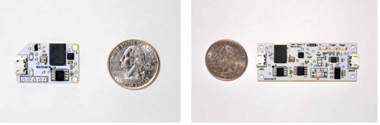
(a) Shoe sensor (b) Region and lesson tracker

Figure 3-1: Shoe sensor and region/lesson tracker PCBs

Each sensor measures the RSSI of incoming data packets to estimate proximity. Shoe sensors approximate social interaction by the transmission of data. Region tracker sensors sense where children spend their time through proximity. The Montessori classroom is organized spatially by curriculum area, so region trackers can approxi-mate time spent on a given subject. Lesson tracker sensors measure how much time students are spending near a lesson.

Figure 3-1a shows the shoe sensor: a 2 x 2.5 cm PCB with a system-on-chip Simblee Bluetooth transceiver radio integrated circuit, a real-time clock (RTC), an accelerometer, microphone, and external flash memory. The system-on-chip contains a 32-bit ARM Cortex-M0 processor with 128 KB of flash memory and 24 KB of RAM. The external flash memory provides 256 KB of storage. Sensors feature a micro-USB port for recharging through a power strip. Sensors are powered by 90 mAh recharge-able lithium-polymer batteries, enclosed in a custom made plastic enclosure for safety. I assembled sensors using standard hand-soldering and reflow oven techniques.

The region tracker and lesson tracker sensors, illustrated in Figure 3-1b, use the same PCB, but run different firmware. A motion-sensing accelerometer enables the lesson tracker to sleep while the lesson is not in use and scan its surroundings for other nodes when a student picks up the lesson tray. These sensors are powered by 1000 mAh rechargeable batteries so they can remain in the classroom for a longer amount of time without recharging.

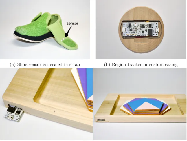
(a) Shoe sensor concealed in strap (b) Region tracker in custom casing

(c) Lesson tracker in tray

Figure 3-2: Sensors are placed in a minimally invasive fashion.

Figure 3-2a shows how shoe sensors are worn inside the shoe strap. The shoe strap firmly holds sensors in place and conceals them from sight. A custom enclosure, attached to shelves in the classroom, houses region trackers without drawing any attention from the children, as shown in Figure 3-2b. Similarly, Figure 3-2c illustrates how sensors fit in the lesson trays in a concealed manner.

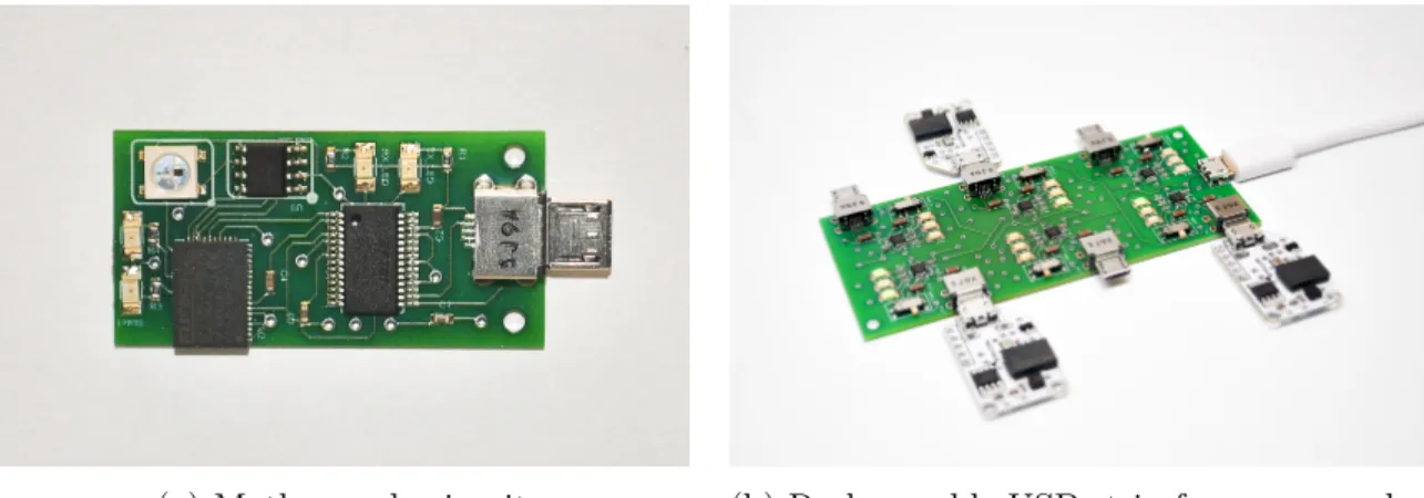
Sensor nodes communicate to a cellphone app through a mother node. The mother node PCB, shown in Figure 3-3a, has the same Simblee Bluetooth transceiver IC and allows UART communication from the microprocessor to a cellphone that has OTG host capabilities. All sensors recharge through a custom designed USB recharging strip, highlighted in Figure 3-3b.

Shoe sensors, region trackers, and lesson trackers transfer their data through a mother node to a cellphone application. The cellphone application then posts this

(a) Mother node circuit (b) Rechargeable USB strip for sensor nodes

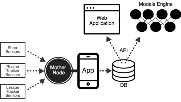
Figure 3-3: Through a mother node, an app controls the rechargeable sensors. data to a centralized database that provides an API. This API powers both the web application and further analytics through a statistical modeling engine. Figure 3-4 illustrates the system diagram.

3.2

Sensor Firmware

The sensor firmware is implemented using the Arduino open-source electronic proto-typing platform [1]. The firmware is uploaded to sensors through a custom cable that connects a computer’s USB bus to the board’s programming leads. I implemented two libraries to enable timekeeping using a software clock and memory management functionality. The firmware utilizes an open-source timekeeping library to interface with the sensor’s RTC. The main components of the firmware are the following:

∙ A distributed sensor network protocol to sense proximity and establish interac-tion context through mointerac-tion and ambient sound data of nodes in the network ∙ A synchronized network event scheduling scheme to establish a shared time

basis and collect data in a battery efficient fashion at a high time resolution for social interaction

∙ A wireless data transfer protocol to facilitate data collection from the network in teacher-friendly manner

Figure 3-4: Sensei system diagram

Together, these components work together to gather sensory data from the class-room while supporting long battery life and providing a teacher-usable interface.

3.2.1

Sensing Proximity and Motion

The Simblee transceiver radio provides a set of libraries to interface with its Bluetooth capabilities. I utilize the SimbleeCOM mesh-networking protocol for data communi-cation. This protocol allows sensors to communicate in a mesh-network with a node to node transmission time of 3 milliseconds.

To capture proximity data, each sensor in the network repeatedly transmits a data packet containing the device’s unique identifier and pauses for a small randomly sized delay. After collecting packets from other sensors, each node records an entry for each device that sent a packet. These entries contain the sender’s device identifier, the mean RSSI of all packets received from a given sender, and a timestamp. Due to constrained memory on each sensor, I use bit shifting to store all three pieces of information in one 4-byte entry. Each proximity entry is structured with form 𝐷𝐷𝑅𝑅𝐻𝐻𝑀 𝑀 𝑆𝑆, where 𝐷 is the device identifier, 𝑅 is the mean RSSI, and 𝐻, 𝑀 , and 𝑆 are the hour, minute, and second components of the timestamp respectively.

Sensor 1 Sensor 2 Sensor 3 Sensor 4 Sensor 5 S S S S S S S S S S S S S S S S S S S S S S S

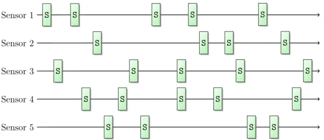
Figure 3-5: Data transmission scheme diagram

The resulting data set is a time series identifying when a student is in proximity to another student or to another region/lesson tracker sensor.

Since the Simblee transceiver only has one radio, each sensor can only send or receive data at any given instant. As a result of this hardware constraint, nodes in the network cannot continuously transmit and receive data. To circumvent this limitation, I implemented a scheme for data transmission based on randomly sized delays. A deterministic approach to this problem is challenging because fixed delay intervals can cause multiple radios to transmit at the same time, leading to repeated transmission collisions and missed data readings.

Figure 3-5 illustrates the data transmission scheme between 5 sensors. The boxes represent the 3 millisecond window of time to send (S) one packet. The unoccupied space between the send intervals represents the time at which the transceiver radio is available to receive data. When a sensor sends its device identifier, other sensors in proximity receive the transmission, only if not transmitting concurrently. Since the pseudo-random number generator used to create the delays is seeded by noise from an unconnected pin on each sensor, each node draws different delay sizes between consecutive data transmissions.

Tests in a laboratory environment verify that delays that vary uniformly at random between 5 and 50 milliseconds maximize the number of instances at which nodes are mutually available to communicate. Although this scheme works well in practice, with

up to clusters of 10 sensors, on occasion there are collisions where multiple radios are transmitting at the same time. For example, in Figure 3-5, there is an instance where both Sensor 3 and Sensor 4 are sending a packet simultaneously. When this occurs, these sensors do not detect the presence of the other and the pairwise relationship is not captured in the recorded data set. I evaluate how well the system captures data successfully in Chapter 5.

The Simblee transceiver supports data transmission up to 100 meters. I tuned the radio transfer power level such that nodes can only transmit data up to three to four feet away, the proximity range of young children engaging in social interaction as found in manual observations. To determine this setting, I tested sensors at different power levels in the classroom environment while varying distance and recording the measured RSSI with different physical obstructions. In test environments, I found that a transmission power level of -12 dBm satisfied the proximity criteria under most conditions. In Chapter 5, I evaluate how well proximity maps to social interaction.

To capture motion data, sensors poll their accelerometer between data trans-missions. After the data collection window, sensors record the mean accelerometer measurement for each spatial axis.

3.2.2

Synchronized Network Event Scheduling Scheme

Network time synchronization is vital to achieving long battery life. All nodes must have their radios active at the same time in order to transmit data, but keeping the radio alive for extended periods is battery inefficient.

Time synchronization is a difficult problem in sensor networks. Nodes do not maintain the global time with precision by default. The standard Arduino library provides facilities to delay code execution and check the number of milliseconds a device has been running. These tools alone, while useful for time insensitive tasks, do not ensure millisecond precision network timing. The sensor’s RTC provides a 1 Hz interrupt and standard timekeeping capabilities with ±5 ppm timekeeping accu-racy. The interrupt cannot be used alone to maintain the time through an interrupt service routine because occasionally the interrupt signal can fail, leading to incorrect

Microprocessor and Radio State Current Expenditure (mA)

Sleep 0.005

RTC Interrupt Service Routine 0.2 Active Microprocessor 4.1

Active Radio 10 - 19.8

Table 3.1: Current expenditures of various microprocessor and radio states Transfer Power Level (dBm) Current Expenditure (mA)

4 19.8 0 14.6 -4 12.5 -8 11.5 -12 10.8 -16 10.3 -20 10

Table 3.2: Current expenditures of running the transceiver radio at various transfer power levels

timekeeping in the network.

Table 3.1 describes the current expenditures of various microprocessor and radio states. While the microprocessor is sleeping, 0.005 mA is drawn. The cost of each interrupt firing is 0.2 mA. The cost of probing the RTC hardware timer is the current required to keep the microprocessor alive, approximately 4.1 mA. When the Bluetooth radio is active, 10 - 19.8 mA is drawn, depending on the transfer power level. Table 3.2 describes the maximum current costs of running the transceiver radio at various transfer power levels.

Due to the hardware limitations and the given costs of various operations, I de-signed a scheme that leverages the accuracy of the RTC hardware clock and the power efficiency of RTC interrupt. In this scheme, the hardware clock is used to synchronize a software clock to the correct time. This synchronization occurs once every ten seconds, when the microprocessor must be active for data collection. After synchronizing the software clock and collecting data, the software clock is driven by the 1 Hz interrupt while the microprocessor sleeps. This scheme ensures the correct-ness of the time when the microprocessor wakes for data collection while allowing for timekeeping while the microprocessor sleeps.

Interrupt

t = 0 t = 1 t = 2 t = 3

RTC Clock

Time Probe Probe XXX Bluetooth Radio XXX S/R XXX

Accelerometer XXX Read XXX Microphone XXX Read XXX

Flash Memory XXX W XXX

Sleep XXX Sleep Sleep Sleep Figure 3-6: Synchronized network event schedule timing diagram

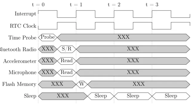
Figure 3-6 illustrates one cycle of the data collection process. Let time 𝑡 be the second component of the software clock modulo 10. The RTC 1 Hz interrupt fires 500 milliseconds out of phase with the rising edge of the RTC time. During data collection, at 𝑡 = 0, sensors wake from sleep and probe the RTC for the rising edge of the following second for approximately 500 milliseconds. Then, the transceiver radio sends and receives (S/R) packets from other nearby sensors as defined by the data transmission scheme. Sensors read the accelerometer and microphone between data transmissions. After 500 milliseconds, nodes record the mean RSSI of each nearby sensor and metrics for the magnitude of the student’s motion and ambient sound volume. After writing data (W), sensors return to a low-power sleep mode until the next cycle of data collection. Sleeping ensures a longer battery life for the sensors, while maintaining a data sampling rate of 10 seconds.

The power efficiency underlying this scheme enables shoe sensors to run for up to 2 school days on a rechargeable 90 mAh battery. Lesson and region tracker sensors run for up to 20 days on a 1000 mAh rechargeable battery. When new sensors are introduced in the existing network, they receive the current time from other nodes and stay synchronized through the event scheduling scheme.

real-time network status tracking, and wireless data collection. For data collection, the mother node receives the current time from the cellphone application through UART serial communication. The mother node shares the current time with all other sensors in the network through Bluetooth, leveraging the fast 3 millisecond data transmission time. The mother node then relays to the cellphone application which sensors are currently active.

3.2.3

Wireless Data Transfer Protocol

Once the sensors have collected data, the teacher retrieves the data in the network. Teachers initiate this process through a cellphone connected to a mother node sensor. The cellphone application and the mother node exchange data through UART serial communication. The mother node communicates with other sensors through Blue-tooth. The mother node requests the contents of each device’s memory, until each device acknowledges a successful data transfer. Each sensor’s flash memory is struc-tured as a set of 1 KB pages. Each page contains 240 4-byte entries, each representing proximity or motion data.

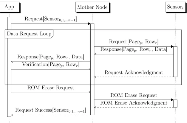
Figure 3-7 illustrates the sequence diagram of the wireless data transfer protocol. First, the cellphone application sends the mother node the set of sensors to collect data from, 𝑅𝑒𝑞𝑢𝑒𝑠𝑡[𝑆𝑒𝑛𝑠𝑜𝑟0,1,...𝑛−1]. Let 𝑆𝑒𝑛𝑠𝑜𝑟𝑖 denote any sensor in this set. The mother

node sends 𝑅𝑒𝑞𝑢𝑒𝑠𝑡[𝑃 𝑎𝑔𝑒𝑝, 𝑅𝑜𝑤𝑟], a request with parameters 𝑃 𝑎𝑔𝑒𝑝 and 𝑅𝑜𝑤𝑟, the

page and row to start the transfer from. Then, 𝑆𝑒𝑛𝑠𝑜𝑟𝑖streams all rows on 𝑃 𝑎𝑔𝑒𝑝from

𝑅𝑜𝑤𝑟onward, denoted 𝑅𝑒𝑠𝑝𝑜𝑛𝑠𝑒[𝑃 𝑎𝑔𝑒𝑝, 𝑅𝑜𝑤𝑟, 𝐷𝑎𝑡𝑎]. The mother node relays each

response packet to the app when it is received. As the app receives each data entry, it verifies that the data is well-formed and satisfies the last request sent by the mother node. This verification, 𝑉 𝑒𝑟𝑖𝑓 𝑖𝑐𝑎𝑡𝑖𝑜𝑛[𝑃 𝑎𝑔𝑒𝑝, 𝑅𝑜𝑤𝑟], is required because occasionally

data is loss over the serial port. If the app detects a discontinuity in the data stream or a malformed data entry and verification fails, then the app resets the data transfer page and row parameters to resume the transfer from the last well-formed entry. Otherwise, this data requesting process repeats with the mother node requesting the next page from 𝑆𝑒𝑛𝑠𝑜𝑟𝑖. Once the last page containing data is sent, the 𝑆𝑒𝑛𝑠𝑜𝑟𝑖

App Mother Node Sensor𝑖

Request[Sensor0,1,...𝑛−1]

Request[Page𝑝, Row𝑟]

Response[Page𝑝, Row𝑟, Data]

Response[Page𝑝, Row𝑟, Data]

Verification[Page𝑝, Row𝑟]

Request Acknowledgment Data Request Loop

Data Request Loop

ROM Erase Request

ROM Erase Request ROM Erase Acknowledgment Request Success[Sensor0,1,...𝑛−1]

Figure 3-7: Wireless data transfer protocol sequence diagram

acknowledges that the last page was transferred in 𝑅𝑒𝑞𝑢𝑒𝑠𝑡 𝐴𝑐𝑘𝑛𝑜𝑤𝑙𝑒𝑑𝑔𝑚𝑒𝑛𝑡. This concludes the data transfer process.

Sensors must be erased to ensure that they are available to collect data for the following school day. I incorporate this process into the wireless data transfer pro-tocol through a remote ROM erase procedure. If 𝑆𝑒𝑛𝑠𝑜𝑟𝑖 acknowledges the end

of the data transfer and verification is successful, the app sends a request to the mother node to remotely erase 𝑆𝑒𝑛𝑠𝑜𝑟𝑖. The mother node forwards this request

to the sensor and the sensor acknowledges that its ROM was successfully erased in 𝑅𝑂𝑀 𝐸𝑟𝑎𝑠𝑒 𝐴𝑐𝑘𝑛𝑜𝑤𝑙𝑒𝑑𝑔𝑚𝑒𝑛𝑡. To conclude the data transfer procedure, the mother node returns a success code for each device that the app originally requested data from in 𝑅𝑒𝑞𝑢𝑒𝑠𝑡 𝑆𝑢𝑐𝑐𝑒𝑠𝑠[𝑆𝑒𝑛𝑠𝑜𝑟0,1,...𝑛−1].

Since Bluetooth is prone to data corruption and packet loss, requests and responses can be dropped in communication at any step in this protocol. Additionally, data is occasionally lost during serial communication. My implementation of this protocol does not assume that any individual packet or serial communication is successful.

(a) Collect data page (b) View data page

Figure 3-8: Cellphone application page for collecting and viewing data

To achieve this functionality, senders dispatch repeated requests in the event that a transmission is unsuccessful or the receiver is unresponsive. To prevent infinite loops while a sender is waiting for a response, I implemented timeouts when a message receiver may not be available. This functionality ensures the robustness of the wireless data transfer protocol under real-world conditions.

In classroom deployments, the time to transfer one page of data is 1,920 millisec-onds. This transfer rate equates to one day of data, approximately 30 pages, typically requiring 60 seconds to wirelessly transfer from the node to the cellphone application.

3.3

Cellphone Application

To use Sensei, teachers interface with the network through a cellphone application. The cellphone app streamlines the process of using the network.

3.3.1

Starting the Network

At the beginning of each day, a teacher starts the network with a single button press. The teacher is presented with a real-time view of which sensors are currently active in the classroom. The teacher places each recharged sensor into the designated shoe of each child.

When the teacher starts the network, the mother node sends the current time to each sensor in the classroom. The time is transmitted at the rising edge of the seconds component of the mother node’s RTC clock. The transceiver’s fast transmission time ensures that sensors receive the time quickly and uniformly.

Upon receiving the time, the sensors acknowledge receipt by transmitting their device identifier to the mother node for 60 seconds. This provides a window of time for the mother node to detect that each sensor in the classroom was properly activated.

3.3.2

Collecting Data

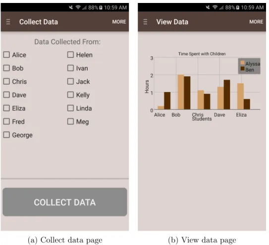
The teacher is presented with a seamless experience for data collection. Figure 3-8a shows the screen where teachers can collect data from the sensors. After pressing the Collect Data button, the app initiates wireless data collection and the teacher sees a progress bar for the process. When the app receives all of the data from a sensor, a box is checked for the corresponding student. When the cellphone receives data from all sensors, the phone sends the data to a secure database.

3.3.3

Viewing Data

After data collection, the teacher views a visualization of their time spent with each child. Figure 3-8b is a time distribution visualization of the collected data. Initial teacher interviews indicated that this graph would be the most helpful to the teachers as they can adjust their methods to address each individual child more equally. This screen is populated with the data that has been most recently collected by the cell-phone application. The web application allows teachers to explore the data in greater depth.

Figure 3-9: Stacked bar chart visualization

3.3.4

Checking Sensor Battery Life

The cellphone application allows teachers to check the battery life of the sensors in their classroom. The app reports the battery life of each sensor.

Each sensor computes an approximation of its battery life. This approximation is computed by tabulating how long the sensor spends in each of the microprocessor and radio transfer power level states in Tables 3.1 and 3.2. Based on the worst-case current expenditures for each state and given the sensor’s rated battery capacity, sensors approximate their battery life percentage.

3.4

Dashboard and Visualizations

Teachers access a classroom summary and data visualizations from an online web application. By logging in with their account credentials, they can view their data

Figure 3-10: Sankey chord visualization for their students.

3.4.1

Visualizations

Sensei provides six visualizations to quantify social interaction, region interaction, and lesson interaction. Researchers in the Social Computing group developed these visualizations using D3.js, a JavaScript library for manipulating data-driven docu-ments.

We have constructed three visualizations to show social interaction in the class-room, varying time dimensions as well as visualization techniques. Figure 3-9 shows a stacked bar chart where teachers select a student from a dropdown menu and view

that student’s interaction with other students in the class. The stacked bar chart highlights periods when students are clustered together. This visualization clearly illuminates the periods when the shoes are returned to a shoe rack at the start and end of the school day. Teachers can identify patterns during other scheduled group activities.

Figure 3-10 shows connections between students over a day of activity. This visualization shows how much time students spend together through the thickness of each chord, allowing teachers to get a sense for aggregate interaction.

To reveal which students teachers spend the least time with, we created a visual-ization, shown in Figure 3-11. This shows the percentage of time two teachers spent with their students, so they can adjust accordingly. The overlapping area shows how a teacher distributes their time with respect to the other teacher.

Figure 3-12 shows the interaction data gathered from the region tracker sensors. As teachers hover over an active area of the classroom, they can see which students spend the most time there. Montessori classrooms are arranged by subject material, so a teacher can immediately see a student’s particular attention to a given subject. We can visualize how long one student spends time with a lesson, as shown in Figure 3-13. Teachers can see a spike when the lesson is introduced and can use this to determine when a child has mastered a lesson. They can use this data to decide when someone is ready to be shown a new lesson.

The accelerometer collects motion data that can be used to understand and clus-ter activity profiles of students in the classroom. Figure 3-14 shows a visualization that shows velocity profile charts for different students. By numerically integrating the acceleration data and calculating the magnitude of velocities over discrete time periods, we can create a histogram visualization that informs teachers about students who are particularly active on a day.

Figure 3-12: Classroom heatmap visualization

Chapter 4

Data Analysis

Sensei produces a time series identifying when a student is in proximity to another student or to another region/lesson tracker sensor. In this chapter, I present the following analysis of the data set:

∙ Distribution of time students and teachers spent in proximity ∙ Distribution of time students spent in classroom regions

4.1

Time Spent in Proximity

To compute how much time students spent in proximity, I applied known time series analysis techniques. The social interaction time series data set contains 15 days of data collected over a 6 week time period. Each day contains approximately 4 hours of data for each student and teacher present in class on the given day. I tabulated the amount of time each student spent with other students by assigning 10 seconds for each entry a student’s sensor recorded.

Figure 4-1 illustrates the distribution of time students and teachers spent in prox-imity. Consider a square 𝑠(𝑖, 𝑗) in the 𝑖𝑡ℎ row and 𝑗𝑡ℎ column in the distribution matrix. The color of the square 𝑠(𝑖, 𝑗) corresponds to the amount of time in hours that the 𝑖𝑡ℎ individual spent with the 𝑗𝑡ℎ individual.

Distribution of Time Spent in Proximity

This figure reveals the approximately symmetric property of the data collected, where 𝑠(𝑖, 𝑗) ≈ 𝑠(𝑗, 𝑖). Since the sensors transmit data in a mesh network, all proxim-ity measurements should occur in pairs. Loss or corrupted data causes discrepancies in the symmetry of the time distribution matrix. I quantity the extent to which data loss impacts the pairwise nature of the data in Chapter 5.

Figure 4-2 represents the normalized time distribution, the data presented in Fig-ure 4-1 where each row is normalized by the length of data contained in that row. The color of a square 𝑠(𝑖, 𝑗) corresponds to the percentage of time that the 𝑖𝑡ℎ

indi-vidual spent with the 𝑗𝑡ℎ individual. The 𝑖𝑡ℎ row illustrates how the 𝑖𝑡ℎ individual spent their time with others in the classroom. The normalized data is not symmetric because the length of the data represented varies across different sensors.

The normalized data reveals how distributions vary across different individuals and allows for comparison of how people spent their time with others. For example, the matrix shows that most individuals spent a disproportionate amount of time with Student 7. The evolution of the time distribution matrix can provide insight into how friendship structures develop and information propagates through a classroom.

4.2

Student Time Spent in Classroom Regions

I computed the distribution of how student spent their time in different regions of the classroom. This distributed was tabulated by assigning 10 seconds for each instance a region tracker registered the presence of a student in proximity. The data set for this computation is a subset of the students and region trackers for one day.

Figure 4-3 illustrates the normalized distribution of student time spent in class-room regions. Consider a square 𝑠(𝑖) in the 𝑖𝑡ℎ _{row in the distribution matrix. The}

color of the square 𝑠(𝑖) corresponds to the percentage of time that the 𝑖𝑡ℎ individual spent in the region of the corresponding column.

Figure 4-4 represents the data in Figure 4-3 aggregated over the entire classroom. This figure shows how actively classroom regions are being utilized. More longitudinal data can reveal how various elements of the classroom are utilized over time.

Normalized Distribution of Time Spent in Proximity

Normalized Distribution of Student Time

Spent in Classroom Regions

Classroom Region Language Shelf

Snack Table

Practical Life Shelf

Sensorial Work Shelf

Snack Shelf Sensor ID 1 2 3 4 5 6 7 8 9 10 11 12 13 Percentage 0 10 20 30 40 50 60 70 80

Classroom Region

Language Shelf

Snack Table

Practical Life Shelf

Sensorial Work Shelf

Snack Shelf

Mean Percentage of Student Time Spent

0

5

10

15

20

25

30

Mean Percentage of Student Time

Spent in Classroom Regions

Classroom Region

Chapter 5

Evaluation

To evaluate Sensei, I conducted the following three studies:

∙ A system robustness analysis in laboratory and school settings ∙ A proximity analysis using manual video annotation

∙ A qualitative usage observation with Montessori educators

These studies characterize the system and help evaluate its use cases. Researchers from the Social Computing group helped conduct the proximity analysis and the usage observation studies.

5.1

System Robustness Analysis

The goal of the system robustness analysis is to quantify how reliably sensors capture proximity. I employ the following metrics to quantify how well the sensors track proximity:

∙ The mean number of packets transmitted ∙ The frequency of detection of nodes in a cluster ∙ The frequency of pairwise sensor detection

Packets Received 0 5 10 15 20 25 Probability 0 0.02 0.04 0.06 0.08 0.1 0.12 0.14 0.16

0.18

Normalized Distribution of Packets Received

Shoe Sensors (n = 82,680) Region Trackers (n = 43,310)

Figure 5-1: Normalized distribution of packets received by shoe sensors and region trackers

These metrics objectively quantify how well the hardware and firmware capture proximity. The mean number of packets transmitted signifies the mean number of data points averaged to compute the mean RSSI for each proximity measurement. The frequency of detection of nodes in a cluster characterizes the percentage of instances that a sensor detects the presence of other nodes in a cluster. The frequency of pairwise node detection measures how consistently pairs of sensors detect each other in proximity.

5.1.1

Proximity Study in Laboratory Setting

To measure how well the shoe sensors capture proximity, a cluster of five shoe sensor nodes were placed within social interaction range in a laboratory setting. Region

trackers were placed near the cluster to measure how well they gauge proximity. Instead of recording RSSI, the sensors tracked the number of packets received from all other nodes. All five shoe sensors collected packet count data for approximately 12 hours and accumulated a total of 𝑛 = 82, 680 packets. The region tracker nodes ran for roughly 25 hours and amassed a total of 𝑛 = 43, 310 packets.

Figure 5-1 represents the normalized packet count distributions of the shoe sensors and the region trackers respectively. Shoe sensors collected a mean of 4.6 packets during each 500 millisecond window. The region tracker nodes collected a mean of 7.6 packets during each window. Shoe sensors detected the presence of other nodes with a probability of 𝑃 𝑟{𝑃 𝑎𝑐𝑘𝑒𝑡𝑠 𝑅𝑒𝑐𝑒𝑖𝑣𝑒𝑑 > 0} = 95.98% and region trackers detected other nodes with a probability of 𝑃 𝑟{𝑃 𝑎𝑐𝑘𝑒𝑡𝑠 𝑅𝑒𝑐𝑒𝑖𝑣𝑒𝑑 > 0} = 99.75% of the time. Region trackers collected more packets and have a greater probability of detecting the presence of other nodes in proximity because the transceiver only listens for nearby sensors, while shoes sensors are both sending and receiving data during the same window of time. Given that sensors sample data every 10 seconds, a low likelihood of missing a single data point does not affect the quality of the data. The probability of not capturing a prolonged interaction between students diminishes with the length of the interaction.

5.1.2

Data Transmission Study in School Setting

In the mesh network, each sensor sends data to all other sensors in proximity. Let the directed graph 𝐺𝑡 = (𝑉, 𝐸), be the graph representing the mesh network where

𝑉 = {𝑣1, 𝑣2, . . . , 𝑣𝑁} is the set of vertices or sensors and 𝐸 = {𝑒1, 𝑒2, . . . , 𝑒𝑀} is

the set of directed edges or data transmissions during a given time range 𝑡. Let each directed edge 𝑒 = {𝑖, 𝑗} represent a data transmission from sensor 𝑖 to sensor 𝑗. Theoretically, every directed edge in 𝐺 should have a corresponding back edge, ∀ 𝑒 = {𝑖, 𝑗} ∈ 𝐸, ∃ 𝑒 = {𝑗, 𝑖} | 𝑖 ̸= 𝑗. Under real-world conditions, data loss or corruption results in missing edges from the graph.

To measure the frequency of pairwise sensor detection, I performed time series analysis on data collected from deployment in one Montessori school. I analyzed 8

Adjacent Time Window (Seconds) Frequency of Pairwise Detection

0 93.51%

10 96.76%

20 97.57%

Table 5.1: Frequency of pairwise detection of sensors in proximity

days of data each containing approximately 4 hours of proximity measurements. The data set contained a total of 𝑛 = 119, 715 data transmissions.

To determine if a transmission at time 𝑡 had a corresponding back transmission, I considered the set of transmissions in the range 𝑡 − ∆𝑡 ≤ 𝑡 ≤ 𝑡 + ∆𝑡 where ∆𝑡 is a window of time and multiple of the network’s sampling rate of 10 seconds. The purpose of the window of time is to allow for a degree of flexibility in detecting whether a back edge exists.

Table 5.1 highlights the frequency of pairwise detection of data transmission in the network for various time windows. I define the frequency of pairwise detection, 𝑓𝑝𝑎𝑖𝑟𝑤𝑖𝑠𝑒, to be the ratio of directed edges with back edges to the total number of

directed edges. For ∆𝑡 = 0 seconds, 𝑓𝑝𝑎𝑖𝑟𝑤𝑖𝑠𝑒 = 93.51%. For ∆𝑡 = 10 seconds and

∆𝑡 = 20 seconds, the frequency increases to 96.57% and 97.57% respectively. This result confirms that Sensei captures approximately symmetric proximity data.

5.2

Proximity Analysis

One limitation of this system is that proximity does not always represent social inter-action. A typical Montessori classroom encourages social interaction among children. To determine how often children are actually interacting, as opposed to simply being in proximity to one another, I studied how well proximity maps to social interaction. I quantified how often these interactions happen on a typical day. I recorded four hours of video in one school that has 3 - 6 year old children. Other researchers from the Social Computing group helped manually annotate the video and record timestamps when children spent more than 10 seconds interacting with one another. We recorded when children were in close proximity and whether they were interacting.

To imitate the sensor network configuration, brief interactions lasting less than ten seconds of proximity were ignored in the manual annotation. Using aggregate values of social interaction and proximity durations, we found that children were actually engaged in interaction 84.9% of the time when they were in proximity to one another. By tracking patterns over time and gathering more longitudinal data, we can help alleviate this limitation of the system.

5.3

Usage Observation

In order to determine the usefulness of Sensei, two other Social Computing researchers and I conducted usage observations in Montessori environments and user interviews with Montessori teachers. Teachers were inclined to talk about the effects of the system, rather than give specific feedback on the usability of the visualizations. We found that teachers used Sensei for the following three use cases:

∙ To augment their manual observations with data ∙ To track learning in their classrooms

∙ To identify needs for increased interaction

We interviewed teachers to validate our hypotheses about how Sensei would be useful. In constructing the visualizations, we determined the expected use of the data and this study helped us validate those use cases. We interviewed teachers to identify shortcomings of the system, which has informed much of our future work.

Our participants were 10 teachers from three types of classrooms: ages 1.5 - 3, ages 3 - 6, and bilingual schools. Teachers were shown five of the different types of visualizations discussed in Chapter 3 to determine their usefulness to their class-room. All visualizations contained anonymized data to encourage teachers to reflect on the system, rather than individual students. We recorded video of the 30 minute interviews, capturing both the teachers’ interaction with the visualizations and their comments.

5.3.1

Augmenting Manual Observations with Data

Overall, the teachers were very interested in being able “to have specific quantifying elements” to augment their manual observations. Every teacher commented on the ability of the sensor network to capture what they are unable to observe in the classroom and felt that the system would help them improve their own methods.

One teacher from a 3 - 6 year old classroom said that this data would be partic-ularly useful for her, as her classroom is divided with walls. Another teacher from a 1.5 - 3 year old classroom mentioned that this data would be especially helpful for younger students. Younger children are often more inclined to abandon lessons, rapidly move to different regions of the room, and socialize. These classrooms are even more difficult to observe, and teachers are usually more active in the classroom, restricting their time to record notes. Another teacher commented that this system “would be especially meaningful around parent-teacher check-in time”, as they can now have more meaningful conversations about the children.

Although Montessori teachers are hesitant about using traditional technology like tablets in the classroom, they were not concerned about Sensei. The system did not substantially change the experience in the classroom during the day. Students rarely recognized the sensors in the classroom.

5.3.2

Tracking Learning

Teachers from 3 - 6 year old classrooms were interested in the data gathered from sensors located around the room and on lesson trays. This information can assist teachers in determining what to introduce to children to further learning outcomes in the classroom.

When shown the lesson usage visualization, Figure 3-13, teachers who taught older children were interested in using this to inform their weekly lesson planning. They were interested in this data to advise them when they should introduce a new lesson into the classroom: “if these lessons aren’t being used at all, then my class is done with them”. Teachers who taught the 1.5 - 3 year old classrooms were less interested

in the data, as children of that age spend less time working on specific lessons. Teachers were interested in identifying a child’s specific interest. One teacher described a scenario where a child chooses a lesson, removes it from the shelf, but then returns it when it is too advanced for them. By seeing proximity data from this scenario, they can recognize these often quick interactions and choose to present the lesson to the child.

When shown the classroom heatmap visualization, Figure 3-12, teachers were drawn to the pie chart depicting a child’s time spent in a area of the classroom. For those who taught the 3 - 6 year old classrooms, they remarked on how this information would help them determine when a child should be encouraged to explore a new subject area.

Teachers raised questions on how Sensei can measure a student’s actual focus on a lesson. Although a student might be in close proximity to the lesson, their attention might be divided. This complex problem can be addressed through more comprehen-sive sensory information such as analyzing voice data from the sensor microphone. The current iteration of the sensors do not fully capture the quality of a child’s en-gagement with another child or lesson. With more comprehensive sensory data, we can detect whether a student is working on a specific lesson with greater confidence.

5.3.3

Needs for Increased Interaction

When shown the stacked bar chart visualization, the Sankey chord visualizations, and the radar chart visualization, Figures 3-9, 3-10, and 3-11, teachers were drawn to identifying clusters of children. Nearly every teacher drew comparisons between the visualizations and their own classroom. Teachers were concerned about children who spent more time alone and identified these children as ones they would reach out to. All of the teachers were interested in the data about their own interactions, which reflected our findings in our initial teacher interviews. One teacher reflected on how much time was spent with children: “I need to get these two kids more independent from us. One of the key Montessori principles is independence.” In the bilingual classroom, teachers were interested in seeing which students spent more time with

the Spanish-speaking teacher compared to the English-speaking teacher. With these visualizations, teachers can reflect on their own methods in the classroom.

Chapter 6

Future Work

6.1

Future Work

In the future, I hope to expand the capabilities of Sensei and share this tool with more educators. Some limitations of the system are the inability to robustly differentiate students in proximity from students who are interacting and measure the depth of a student’s engagement with a lesson. Some further extensions of Sensei include the following:

∙ Augmenting the system’s sensory capabilities to better capture social interaction ∙ Measuring the quality of a student’s engagement with a lesson

∙ Developing an interface for parents to view information specific to their child

In order to distinguish proximity from social interaction and quantify the depth of a student’s engagement with their work, sensors will need to capture a more compre-hensive image of student behavior. Other forms of sensory information can include audio-based data such as what a student says and touch-based information such as when a student is in physical contact with lesson materials. A broader set of sensory data can provide enough context to discern proximity from social interaction with high confidence and measure student engagement with lessons. These augmentations

to the system can provide deeper insights into how interaction and learning evolve in early childhood classrooms.

The Sensei API can facilitate early childhood learning research in many different ways. This unique data set can be used to create models of social and learning interaction.

For example, using hidden Markov models, we can classify “hidden states” under-lying children’s learning patterns based on lesson activity [19]. Maria Montessori and other early childhood researchers have observed that children have “sensitive periods” in which they are particularly open to learning a certain subject [13]. Hidden Markov models can help understand and quantify these sensitive periods shown in Figure 6-1a. Given a set of child-lesson dyads, algorithms such as probabilistic latent semantic indexing (PLSI) can uncover latent themes in the curriculum and in sets of children, highlighted in Figure 6-1b [8]. This technique can be extended over multiple schools. Using microphone data, we can create a directed social graph based on who is speak-ing in a cluster. We can analyze this network usspeak-ing PageRank-based algorithms such as eigenvector centrality methods to understand the influence of different children in the classroom represented by Figure 6-1c [7, 17].

(a) Hidden Markov models can quantify

sen-sitive periods. (b) PLSI can infer latent themes in the cur-_riculum.

(c) Eigenvector centrality algorithms can approximate social influence.

Figure 6-1: Algorithms can uncover sensitive periods, latent curriculum themes, and social influence.

Bibliography

[1] Arduino. https://www.arduino.cc/. Accessed: 05-20-2016.

[2] Pulkit Agrawal, Ross Girshick, and Jitendra Malik. Analyzing the performance of multilayer neural networks for object recognition. In Computer Vision–ECCV 2014, pages 329–344. Springer, 2014.

[3] Alain Barrat, Ciro Cattuto, Vittoria Colizza, Jean-Francois Pinton, Wouter Van den Broeck, and Alessandro Vespignani. High resolution dynamical mapping of social interactions with active rfid. arXiv preprint arXiv:0811.4170, 2008. [4] Horesh Ben Shitrit, Jérôme Berclaz, François Fleuret, and Pascal Fua.

Multi-commodity network flow for tracking multiple people. Pattern Analysis and Machine Intelligence, IEEE Transactions on, 36(8):1614–1627, 2014.

[5] Judy Dunn. The emanuel miller memorial lecture 1995 children’s relationships: Bridging the divide between cognitive and social development. Journal of Child Psychology and Psychiatry, 37(5):507–518, 1996.

[6] Paul Epstein. An Observer’s Notebook: Learning from Children with the Obser-vation CORE. Montessori Foundation, 2012.

[7] Taher Haveliwala, Sepandar Kamvar, and Glen Jeh. An analytical comparison of approaches to personalizing pagerank. 2003.

[8] Thomas Hofmann. Probabilistic latent semantic indexing. In Proceedings of the 22nd annual international ACM SIGIR conference on Research and development in information retrieval, pages 50–57. ACM, 1999.

[9] Kourosh Khoshelham and Sander Oude Elberink. Accuracy and resolution of kinect depth data for indoor mapping applications. Sensors, 12(2):1437–1454, 2012.

[10] Suren Kumar, Tim Marks, and Michael Jones. Improving person tracking using an inexpensive thermal infrared sensor. In Proceedings of the IEEE Conference on Computer Vision and Pattern Recognition Workshops, pages 217–224, 2014. [11] Angeline Lillard and Nicole Else-Quest. Evaluating montessori education.

[12] Angeline S Lillard, ON Saracho, and B Spodek. Playing with a theory of mind. Multiple perspectives on play in early childhood education, pages 11–33, 1998. [13] Angeline Stoll Lillard. Montessori: The science behind the genius. Oxford

Uni-versity Press, USA, 2005.

[14] Rossana Mastrandrea, Julie Fournet, and Alain Barrat. Contact patterns in a high school: a comparison between data collected using wearable sensors, contact diaries and friendship surveys. PloS one, 10(9):e0136497, 2015.

[15] Maria Montessori. The montessori method. Transaction Publishers, 2013. [16] Daniel Olguín-Olguín and Alex Pentland. Sensor-based organisational design and

engineering. International Journal of Organisational Design and Engineering, 1(1-2):69–97, 2010.

[17] Lawrence Page, Sergey Brin, Rajeev Motwani, and Terry Winograd. The pager-ank citation rpager-anking: bringing order to the web. 1999.

[18] Deborah A Phillips, Jack P Shonkoff, et al. From Neurons to Neighborhoods:: The Science of Early Childhood Development. National Academies Press, 2000. [19] Lawrence R Rabiner. A tutorial on hidden markov models and selected

applica-tions in speech recognition. Proceedings of the IEEE, 77(2):257–286, 1989. [20] Nazmus Saquib, Ayesha Bose, Dwyane George, Connie Liu, and Sepandar

Kam-var. Sensei: Sensing educational interaction. Submission to UIST 2016, 2016. [21] Juliette Stehlé, Nicolas Voirin, Alain Barrat, Ciro Cattuto, Lorenzo Isella,

Jean-François Pinton, Marco Quaggiotto, Wouter Van den Broeck, Corinne Régis, Bruno Lina, et al. High-resolution measurements of face-to-face contact patterns in a primary school. PloS one, 6(8):e23176, 2011.

[22] Arkadiusz Stopczynski, Vedran Sekara, Piotr Sapiezynski, Andrea Cuttone, Mette My Madsen, Jakob Eg Larsen, and Sune Lehmann. Measuring large-scale social networks with high resolution. PloS one, 9(4):e95978, 2014.

[23] P Bruce Uhrmacher. Uncommon schooling: A historical look at rudolf steiner, anthroposophy, and waldorf education. Curriculum Inquiry, 25(4):381–406, 1995. [24] Julianne Wurm. Working in the Reggio way: A beginner’s guide for American

teachers. Redleaf Press, 2005.

[25] Piero Zappi, Elisabetta Farella, and Luca Benini. Tracking motion direction and distance with pyroelectric ir sensors. Sensors Journal, IEEE, 10(9):1486–1494, 2010.