An integrated simulation method for flash-flood risk assessment: 1. Frequency predictions in the Bisagno River by combining stochastic and deterministic methods

(1)

HAL Id: hal-00304661

https://hal.archives-ouvertes.fr/hal-00304661

Submitted on 1 Jan 2002

HAL is a multi-disciplinary open access archive for the deposit and dissemination of sci-entific research documents, whether they are pub-lished or not. The documents may come from teaching and research institutions in France or abroad, or from public or private research centers.

L’archive ouverte pluridisciplinaire HAL, est destinée au dépôt et à la diffusion de documents scientifiques de niveau recherche, publiés ou non, émanant des établissements d’enseignement et de recherche français ou étrangers, des laboratoires publics ou privés.

assessment: 1. Frequency predictions in the Bisagno

River by combining stochastic and deterministic

methods

M.C. Rulli, R. Rosso

To cite this version:

M.C. Rulli, R. Rosso. An integrated simulation method for flash-flood risk assessment: 1. Frequency predictions in the Bisagno River by combining stochastic and deterministic methods. Hydrology and Earth System Sciences Discussions, European Geosciences Union, 2002, 6 (2), pp.267-284. �hal-00304661�

(2)

An integrated simulation method for flash-flood risk assessment:

1. Frequency predictions in the Bisagno River by combining

stochastic and deterministic methods

Maria Cristina Rulli and Renzo Rosso

Dipartimento di Ingegneria Idraulica, Ambientale Infrastrutture Viarie e Rilevamento, Politecnico di Milano, Piazza L. da Vinci, 32 I-20133 Milano, Italy Email for corresponding author: [email protected]

Abstract

A stochastic rainfall generator and a deterministic rainfall-runoff model, both distributed in space and time, are combined to provide accurate flood frequency prediction in the Bisagno River basin (Thyrrenian Liguria, N.W.Italy). The inadequacy of streamflow records with respect to the return period of the required flow discharges makes the stochastic simulation methodology a useful operational alternative to a regionalisation procedure for flood frequency analysis and derived distribution techniques. The rainfall generator is the Generalized Neyman-Scott Rectangular Pulses (GNSRP) model. The rainfall-runoff model is the FEST98 model. The GNSRP generator was calibrated using a continuous 7-years’ record of hourly precipitation measurements at five raingauges scattered over the Bisagno basin. The calibrated rainfall model was then used to generate a 1000 years’ series of continuous rainfall data at the gauging sites and a flood-oriented model validation procedure was developed to evaluate the agreement between observed and simulated extreme values of rainfall at different scales of temporal aggregation. The synthetic precipitation series were input to the FEST98 model to provide flood hydrographs at selected cross-sections across the river network. Flood frequency analysis of the annual flood series (AFS) obtained from these simulations was undertaken using L-moment estimations of Generalized Extreme Value (GEV) distributions. The results are compared with those determined by applying a regional flood analysis in Thyrrhenian Liguria and the derived distribution techniques to the Bisagno river basin. This approach is also useful to assess the effects of changes in land use on flood frequency regime (see Rosso and Rulli, 2002).

Keywords: flood frequency, stochastic rainfall generator, distributed rainfall runoff model, derived distribution

Introduction

The Bisagno river catchment of approximately 92 km2_is

located in Thyrrenian Liguria, a region in north-west Italy characterised by complex orography, heavy storms, and flash floods. The river valley has experienced rapid urbanisation over the past century as Genoa, the third largest city in the northern Italy, has expanded. To satisfy the increasing need for urban development, narrow channels and dikes have been substituted for natural reaches of the lower river system. Hence, the Bisagno river basin may be considered representative of the interaction between man’s activities and a naturally flash-flood prone environment (Rosso and Rulli, 2002).

Where streamflow data are scarce, simulation techniques can provide useful insights into flood processes; in the Bisagno basin they may be useful in assessing flood frequency in the urban areas. This approach involves the application of a stochastic model of space-time rainfall to perform Monte Carlo simulations of realistic storm fields

over the catchment area. The Generalized Neyman-Scott Rectangular Pulses (GNSRP) model developed by Cowpertwait (1994, 1995) was used because of its ability to represent the high temporal rainfall fluctuations experienced during a storm event, as well as the spatial variability of rainfall rates across the basin area. The spatial pattern, in fact, was observed to play a major role in determining the flood hydrograph at the Bisagno basin outlet. (e.g. La Barbera et al., 1978).

A flood-oriented validation procedure for the GNSRP model which makes use of the observed and simulated scaling properties of storm rainfall is proposed here.

Continuous hourly simulations of the spatially distributed precipitation are input to the spatially distributed physically-based rainfall-runoff model FEST98 (Mancini, 1990), which estimates streamflow across the river network. The FEST98 model allows the essential effects of soil retention, antecedent moisture content and stream flow propagation to be incorporated, although with simplified

(3)

concep-tualisation. Because of the scarcity of observed flood data, the rainfall-runoff model was calibrated considering only the flood event of October 7th_{, 1970, the biggest flood}

recorded in the 20th century at the basin outlet, and was validated successfully using the event of October 20th_{, 1960.}

The rainfall generator and the rainfall-runoff modelling procedures are described in the next two sections, followed by an analysis of synthetic flood data using the GEV distribution. The results obtained are compared with those achieved by statistical regionalisation and derived distribution techniques.

Rainfall generation using the GNSRP

model

METHODOLOGICAL ASSESSMENT

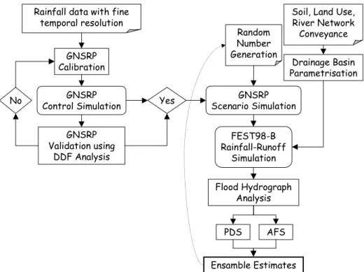
Figure 1 is a flowchart of the methodology to generate hourly precipitation series at the selected locations of the Bisagno basin with the GNSRP model, for subsequent use as inputs to the distributed rainfall-runoff model FEST98. Rainfall depths recorded at five raingauges across the Bisagno basin constitute the data set used for the calibration of the GNSRP model. On the basis of the model parameters, estimated by the method of the moments, synthetic rainfall series are generated by a simulation algorithm, and the model perfomance is evaluated by comparing the statistical

properties of the generated rainfall rates with those of the corresponding rainfall records.Three different simulation scenarios concerning the width of the data set used, the type of rainfall chosen and the different storm regimes co-existing in the basin, are investigated to achieve realistic results in terms of simulated rainfall fields.

While the model cannot preserve the observed statistics over the whole range of temporal scales of aggregation, it provides satisfactory approximations to the basic statistics of the precipitation fields for a range of scales of interest. Hence, a flood-oriented validation procedure may be useful in assessing the capability of the GNSRP model in reproducing storm extremes by comparing simulated and historical rainfall maxima at given sites for different times of aggregation, and for different return periods. Accordingly, depth-duration-frequency (DDF) curves are reproduced from the annual maximum values of simulated rainfall totals, as extracted from the simulated series for selected durations. These DDF curves can be compared with those determined directly by frequency analysis of the observations. If the results are not satisfactory, the model requires a recalibration. The inherent unrobustness of the calibration procedure is associated with the nonlinear optimisation required to determine the parameters, this is highly sensitive to the initial conditions and to the occurrence of local minima of the error function.

Two different historical sample sets are available for model

Rainfall data with fine temporal resolution GNSRP Calibration GNSRP Control Simulation GNSRP Validation using DDF Analysis No Yes FEST98-B Rainfall-Runoff Simulation Flood Hydrograph Analysis GNSRP Scenario Simulation PDS AFS Ensamble Estimates Drainage Basin Parametrisation

Soil, Land Use, River Network Conveyance Random

Number Generation

Fig. 1. Methodological approach scheme to GNSRP calibration, Monte Carlo rainfall simulation, and streamflow generation.

(4)

validation. As a first choice, one can perform frequency analysis on the data set used to calibrate the GNSRP model, using a relatively short record, namely seven years in the Bisagno River case study. The major drawback is its poor capability of providing storm events with large return periods. Cameron et al., (1999) incorporated long term extreme rainfalls in developing their stochastic rainfall model and obtained good results in reproducing rainfall extremes for different durations. Hence, an alternative data set may be constituted by the long-term series of rainfall extremes available in the Hydrology Yearbook published by the Italian Hydrologic Service. Yet, while long records provide more reliable estimates of low probabilities, problems may arise from possible non-stationarity of the underlying physical process due to climate fluctuations. These effects were assessed by De Michele et al. (1998), whose regional analysis based on long-term records of maximum daily precipitation in Italy included data from the Genoa University Station, the records of which are, in part, used in this paper. In the present analysis, both data sets are used and the results are compared and discussed.

Two different probability models can be used to describe the observed scaling properties of maximum rainfall: (1) the Lognormal and GEV simple scaling models, and (2) the Lognormal multiscaling model (Burlando and Rosso, 1996). Note that the influence of the parent statistical distribution is irrelevant for moderate return periods so that the validation process is independent of the underlying statistical model used to analyse the frequency of observed storms. The choice of an appropriate frequency model becomes important for return periods greater than 50 years in the Bisagno River case study. This yields additional uncertainties in validating simulated patterns for extreme storms.

The GNSRP model

The GNSRP model is a further development of the Neyman-Scott Rectangular Pulses (NSRP) model. It was generalised (Cowpertwait, 1994) by allowing different cell types to coexist in the same event and then extended into the spatial domain (Cowpertwait, 1995). Consider a region (or catchment) in the x–y plane. Storm origins arrive in a Poisson process with rate l, the arrival times being the same at any point in the catchment. The arrival of a storm origin at a catchment implies that the physical conditions necessary for rainfall have been met, e.g. a frontal system has arrived at the catchment. However, rain occurs only at points in the catchment covered by rain cells. Each cell can be classed randomly as 1 of n types, with some probability that the cell is of type i (i = 1, ..., n). The radius R is an independent exponential random variable with parameter γ. The intensity

X_I, an independent exponential random variable, remains constant over the area of the disc and throughout the lifetime of the cell; the lifetime is an independent exponential random variable with parameter η. If t is the arrival time of the storm origin and s (>t) is the starting time for a rain cell generated by the origin, then s-t is an independent exponential random variable with parameter _{β, so that the} arrival times of rain cells follows a Neyman-Scott process. The total rainfall intensity at an arbitrary time t and point m is the summation of the intensities of all cells ‘alive’ at time t that overlap point m. As for the single-site model, cells may be classified into different types (e.g. two types: convective and stratiform).

In three-dimensional space, the intensity X_i at a point m with coordinates (x, y, z) is scaled by a factor (which can be a function of the altitude z of the point, to make an allowance for the effects of orography). Furthermore, each cell can have a survival probability of reaching ground level (at low altitudes rain can evaporate before reaching ground level). The k parameters of GNSRP model are listed in Table 1.

As Rodriguez-Iturbe et al. (1987), Onof and Wheater (1993) and Cowpertwait (1994) derived the analytical formulations of the second order statistics of the rainfall process as a function of model parameters, the model can be calibrated using the method of moments. This requires equating k analytical moments with the corresponding sampling moments estimated from the observed time series. This yields a non-linear system of k equations for k unknown parameters. Because an optimisation procedure is required to solve this problem, one accounts, better, for n>k moments to achieve accurate parameter estimates. Denoting with ϕi = ϕi(λ, αi, β, ηi, ξi, γi) a statistical property depending on

the theoretical model parameters, and with ϕˆ_ι _{the sample}

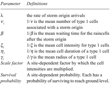
Table 1. Physical meaning of GNSRP model parameters. Parameter Definitions

λ the rate of storm origin arrivals ν1 1/ν is the mean number of type 1 cells

associated with a storm origin

β 1/β is the mean waiting time for the raincells after the storm origin

ξ1 1/ξ is the mean cell intensity for type 1 cells

η1 1/η is the mean cell duration of a type 1 cell

γ1 1/γ is the mean radius of a type 1 cell

Scale factor A site-dependent factor by which the cell intensities are multiplied.

Survival A site-dependent probability. Each has a probability probability of surviving to reach ground level.

(5)

Scoffera

Viganego Sant’Eusebio

Ponte Carrega

sità Ponte Sant’Agata

La Presa

estimate of ϕi, one can obtain a solution by minimising an

objective function, in this case given by a sum of squares. The process of achieving a solution is rather cumbersome even in the one-dimensional case, as shown by Burlando and Rosso (1991). Therefore, the estimation procedure involves a certain degree of subjectivity depending on the algorithm used for optimisation and on the initial conditions needed to perform numerical computations.

Because of seasonal variations in rainfall, one must also account for model parameter variability through the year. To reproduce non-stationarity and/or periodicity of the precipitation field in time, one can fit the model to each calendar month of a rainfall record, resulting in 12 estimates per parameter for each site. To reduce the computational effort, one may assume smooth seasonal variations in the estimated parameters; that is, if φi is a parameter estimate of

the GNSRP model for the i-th month and m_ϕ, Λ_ϕ, θ_ϕ are harmonic parameters, then

      ₊ Λ + = _φ _φ π θ_φ φ 12 2 i sin m i (1)

However, this can oversmooth the rainfall process, so this procedure must be applied carefully if extreme values are to be reproduced.

The values of parameters are estimated by minimising the sum of squares:

∑ ∑ ∑ ∑         − = = = ∈ ∈ m 1 j 12 1 i h Hf F 2 ji ji ji ˆ ) h ( 1 SS ϕ ϕ , (2)

where F is a set of aggregated second-order properties,

ji

ˆ

ϕ denotes the sample estimate of ϕji for the i-th calendar

month at the site j, H is a set of aggregation levels and m is the number of sites considered. The subjectiveness in model calibration is associated with the appropriate choice of the n moments used in the exercise, as there are many possible choices for F and H.

APPLICATION OF THE GNSRP MODEL TO THE BISAGNO RIVER BASIN CASE STUDY

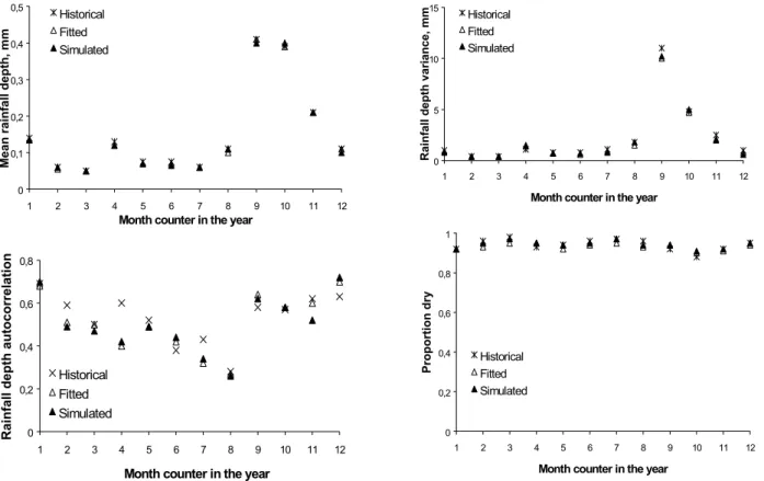
To apply the GNSRP model, from a continuous record of seven years’ (1990–1996) data, four months (September– December) of hourly precipitation totals from five raingauges for each year (Fig. 2) were selected. To reduce the computational effort, just one type of rainfall cell, that is, an elementary precipitation impulse, was assumed to represent the physical unit producing the rainfall patterns. This model, denoted GNSRP(1), was calibrated by the method of moments using two different sets of basic statistics (Table 2). Two estimates for each parameter resulted, with negligible differences between them. The GNSRP model goodness-of-fit was evaluated for each raingauge site by visual comparison at different temporal aggregation levels between the sampling statistics and those derived from the GNSRP model formulation. In terms of mean and variance, agreement was satisfactory but relatively less so in terms of autocorrelation, proportion dry and cross-correlation, indicating the model’s inability to describe accurately the complex fluctuations of the rainfall. Moreover, the proportion dry in rainfall-runoff trans-formation is important

Genova Università

Fig. 2. Raingauge locations and streamflow stations across the

Bisagno River basin.

Table 2. Statistics employed in the estimation of GNSRP model parameters

Dataset 1 Dataset 2 Aggregation level 1 h 3 h 6 h 12 h 24 h 1 h 3 h 6 h 12 h 24 h Mean x X Variance x x x X X X X X Proportion Dry X X X Autocorrelation x x x Cross-correlation x X

(6)

because it controls the antecedent soil moisture conditions. Using these parameter estimates, 1000 years of 1-hour precipitation time series were simulated at each raingauge site. To assess the ability of simulated time series to reproduce the observed statistics, the Student’s t-test was carried out for the second order moments, and an admittance region with 5% confidence level was determined successfully. An extreme value model validation was performed to test model ability in reproducing the observed extreme storms. The maximum annual values of rainfall were extracted from the continuous simulated time series for durations of 1, 3, 6, 12 and 24 hours and from the observed maxima from the Hydrology Yearbook published by the Italian Hydrologic Service. Accordingly, both historical and simulated DDF curves were estimated for return periods of 5, 10, 25, 50 and 100 years. Different statistical distributions (e.g. Lognormal multiscaling distribution, General extreme value simple scaling distribution) were tested to determine which would best fit the observations. The plots of statistical distributions interpolating historical and simulated rainfall maxima showed that Viganego and Scoffera stations were modelled better by a multiscaling lognormal distribution, while Genova Università, Ponte Carrega and S. Eusebio stations, under a marine influence, showed a better agreement with the simple scaling GEV model. Therefore, the intrinsic scaling properties of the observed storm data appear to depend on the major physical factors influencing the storm pattern. This also indicates that a rainfall model should capture multifaceted precipitation structures to mimic the complex pattern displayed by the small-mesoscale precipitation process in the area. The comparison between simulated and historical DDF indicates that Monte Carlo simulations generally overestimate the observed extreme storms for a wide range of scales. This may be due also to the embedded non-stationarity of long-term precipitation in the study area. In fact, the calibration period of the GNSRP(1) model from 1990 to 1996 displays a higher climate activity than over the period of historical extremes considered in the analysis, from the beginning of the twentieth century for some stations. So the estimated GNSRP(1) parameters may describe a climate that differs somewhat from that characteristic of the whole recording period. Non-stationarity symptoms on precipitations were detected by De Michele et al. (1998).

The above results of rainfall field simulation showed that the GNSRP(1) model overestimates the historical extreme values of precipitation for the range of temporal scales of interest in the flash-flood generation process. Therefore, the Monte Carlo rainfall simulation procedure needed to be improved to achieve realistic precipitation inputs. Hence, a

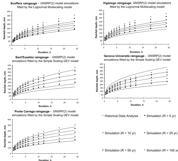
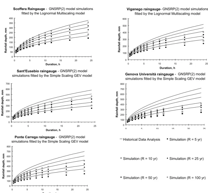
more complete data set was used, with 12 months instead of four months of hourly rainfall totals from 1990 to 1996, as well as two types of raincells (representing convective and stratiform rain, respectively). This model, called the GNSRP(2) model produced results from the fitting procedure that were satisfactory in terms of second order statistics (Fig. 3). However, comparison between historical and simulated DDF curves did not agree so well, because the simulated DDF curves overestimated those from extreme data analysis (Fig. 4). This overestimation is noticeable for the Scoffera and Viganego stations; for the Genoa University station (Fig. 4), overestimation for low-moderate return periods (5 to 10 years) leads to underestimation for high return periods (50 to 100 year). Note that the sampling period (seven years) on which the stochastic model is estimated differs from the much longer period (up to 58 years) used for the DDF analysis of historical data. Comparison of the GNSRP(2)-simulated DDF curves with those derived by analysis of the same seven years’ data from 1990 to 1996 (Fig. 5) displays patterns opposite to the previous ones, as the GNSRP(2)- simulated DDF curve underestimates those obtained from extreme value analysis, particularly for the Ponte Carrega and Genoa University stations. Therefore, the application of the GNSRP(2) model is not a significant improvement on the GNSRP(1), since it underestimates the storm in the lower Bisagno basin, where the largest (artificially) impervious areas are located, and the local hydrological response is very fast. Further, the statistical analysis of a short sample of extreme values (such as the 1990-1996 seven-year sample) cannot capture the extremes for return periods greater than 20 years.

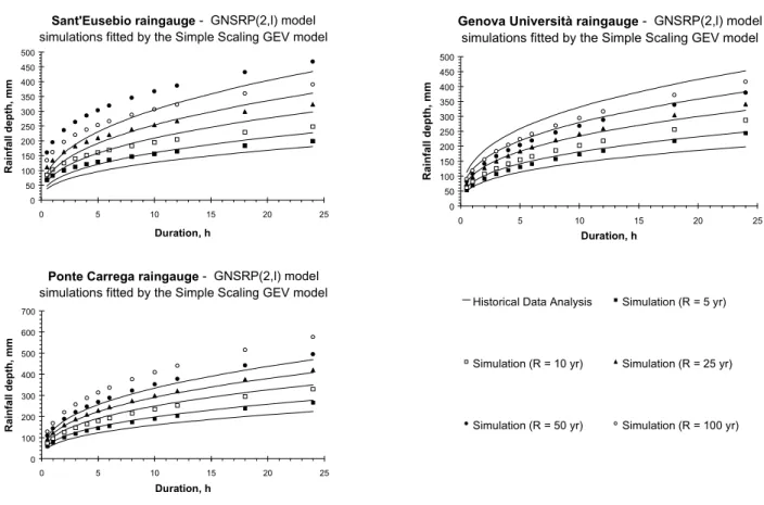
Because of the recognised complexity of the small-mesoscale rainfall patterns investigated, further model refinements can be sought. For instance, two somewhat different storm regimes coexist in the area so that the basin may be subdivided into two separate sub-basins, the lower including the Genova Università, Ponte Carrega and Sant’Eusebio stations, exposed to sea storms, and the upper including the Viganego and Scoffera stations, surrounded by the mountain range. Accordingly, a new calibration and validation session for each basin portion was undertaken; again, historical extreme values were not reproduced any better than previously. Taking into account the whole historical data set (Fig. 6), simulated DDF curves overestimate historical ones for four stations out of five, the exception being the Genoa University station. The simulations for the stations located in the upper part of the basin (namely Scoffera and Viganego) do not look different from those obtained in previous analysis. For Ponte Carrega and Sant’Eusebio stations the new simulation runs look poorer than the previous ones, as reflected by the decreasing

(7)

slope of the simulated DDF in Sant’Eusebio which leads to an increasing overestimation of rainfall for short durations. Figures 8 and 9 were obtained using the DDF curves derived from the 1990 to 1996 data set. Scoffera and Genoa University stations do not display significant changes with respect to the previous analysis. Ponte Carrega shows a fair improvement (the gap between simulated and historical DDF is reduced slightly), while at Viganego station the simulated DDF curves show a reduced slope; consequently, they underestimate historical curves particularly for durations greater than ten hours. The present advances in the GNSRP modelling process are not sufficient to reproduce complex rainfall patterns such as considered in this work. It is difficult to ascribe this drawback to the inherent structure of the model or to the sophisticated mathematical algorithms required for its calibration. The problems with the GNSRP model at this site might also be attributed to the reliance of 1st _{and 2}st_{order statistics (without extremes) in the model}

fitting. In addition, the exponential distribution used for raincell intensity might not be flexible enough to reproduce the different varieties of rainfall intensity in this catchment. Further developments are needed, however, to improve the rainfall generation under orography and climate conditions such as those considered in this paper.

Rainfall-runoff simulation

The second part of the work concerns the application of the distributed rainfall-runoff model named FEST98. The pioneer issue of the FEST model is due to Mancini (1990) and further developments were reported by Mancini et al. (2000), Brath and Montanari (2000) and Kurtner and Burlando (2000). This model uses the continuous precipitation series generated by the GNSRP model for the five gauging sites, specifically obtained by the GNSRP(2) model. As a major requirement to achieve a realistic space-time evolution of basin response to rainfall inputs, the FEST98 model incorporates the Digital Elevation Model (DEM) data of the basin area. These data are provided here in grid based format with elevations averaged on a grid of resolution 7.5” in latitude and 10” in longitude, resulting in 220×230 m2_{rectangular cells. This enables the model to}

represent the drainage basin and its river system accurately without incurring prohibitive computational costs. The spatial distribution of parameters associated with the DEM data structure plays a major role in determining changes in flood occurrence and severity associated with either anthropogenic land use modifications or geomorphological singularities. The distributed characterisation of the flood 0 0,1 0,2 0,3 0,4 0,5 1 2 3 4 5 6 7 8 9 10 11 12

Month counter in the year

Mean rainfall depth, mm

Historical Fitted Simulated 0 5 10 15 1 2 3 4 5 6 7 8 9 10 11 12

Rainfall depth variance, mm

Historical Fitted Simulated 0 0,2 0,4 0,6 0,8 1 2 3 4 5 6 7 8 9 10 11 12

Rainfall depth autocorrelation

Historical Fitted Simulated 0 0,2 0,4 0,6 0,8 1 1 2 3 4 5 6 7 8 9 10 11 12

Month counter in the year Proportion dry Historical_Fitted

Simulated

Fig. 3. Comparison between statistical properties of observed and generated rainfall depths at 1-h time resolution using the GNSRP model.

(8)

dynamics allows reproduction of the hydrograph at any river site, highlighting critical areas particularly subject to flood risk.

The FEST98 model has two major modules (see Fig. 10). The first provides the automatic extraction of the river network from basin topography as given by a rectangular grid-based DEM, identifying the connection between the elemental cells and the related hydrological paths. The second provides hydrological computations for each elemental cell and for the clustered cells throughout the hydrological paths. The extraction of the river network is carried out by first removing local depressions (pits) where flow paths converge from all the adjacent cells. This is generally carried out by increasing local elevations of

depressed cells, so a certain degree of approximation in the representation of catchment topography is introduced (Band, 1986). The network is then identified by assigning to each DEM cell a maximum slope pointer, and then processing each cell to organise the flow path structure based on the steepest slope method. The discrimination between non-channellised and non-channellised cells that determines overland and channel flow, follows the concept of constant critical support area (Montgomery and Foufoula-Georgiou, 1993). Accordingly, overland flow paths are associated with those cells draining an area not exceeding a specified threshold value (0.5 km2_{for this mountain catchment) and}

channellised paths occur otherwise.

Prior to surface hydrology computations, spatial

Fig. 4. Simulated DDF curves compared with those derived from historical data set provided by

Hydrology Yearbook for the five gauging stations.

Genova Università raingauge - GNSRP(2) model simulations fitted by the Simple Scaling GEV model

0 50 100 150 200 250 300 350 400 450 500 0 5 10 15 20 25 Duration, h Rainfall depth, mm

Viganego raingauge- GNSRP(2) model simulations fitted by the Lognormal Multiscaling model

0 50 100 150 200 250 300 350 400 450 0 5 10 15 20 25 Duration, h Rainfall depth, mm

Scoffera raingauge - GNSRP(2) model simulations fitted by the Lognormal Multiscaling model

0 50 100 150 200 250 300 350 400 0 5 10 15 20 25 Duration, h Rainfall depth, mm

Ponte Carrega raingauge - GNSRP(2) model simulations fitted by the Simple Scaling GEV model

0 100 200 300 400 500 600 0 5 10 15 20 25 Duration, h Rainfall depth, mm

Sant'Eusebio raingauge - GNSRP(2) model simulations fitted by the Simple Scaling GEV model

Historical Data Analysis Simulation (R = 5 yr)

Simulation (R = 10 yr) Simulation (R = 25 yr)

(9)

Scoffera Raingauge - GNSRP(2) model simulations fitted by the Lognormal Multiscaling model

Viganego raingauge- GNSRP(2) model simulations fitted by the Lognormal Multiscaling model

Sant'Eusebio raingauge - GNSRP(2) model simulations fitted by the Simple Scaling GEV model

0 100 200 300 400 500 600 700 0 5 10 15 20 25 Duration, h Rainfall depth, mm

Scoffera raingauge - GNSRP(2,u) model simulations fitted by the Lognormal Multiscaling

model 0 50 100 150 200 250 300 350 0 5 10 15 20 25 Duration, h Rainfall depth, mm

Viganego raingauge - GNSRP(2,u) model simulations fitted by the Lognormal Multiscaling

Fig. 5. Simulated DDF curves compared with those derived from the 1990-96 data set provided by Hydrology Yearbook

for the five gauging stations.

Fig. 6. Simulated DDF curves compared with historical ones –Upper part of the basin (Scoffera and Viganego stations).

[Symbols as for Fig. 5]

Ponte Carrega raingauge - GNSRP(2) model

simulations fitted by the Simple Scaling GEV model

(10)

Genova Università raingauge - GNSRP(2,l) model simulations fitted by the Simple Scaling GEV model

Ponte Carrega raingauge - GNSRP(2,l) model simulations fitted by the Simple Scaling GEV model

Scoffera raingauge - GNSRP(2,u) model simulations fitted by the Lognormal Multiscaling

model 0 50 100 150 200 250 300 350 400 0 5 10 15 20 25 Duration, h Rainfall depth, mm

Viganego raingauge - GNSRP(2,u) model simulations fitted by the Lognormal Multiscaling

Fig. 7. Simulated DDF curves compared with historical ones –Lower part of the basin (Sant’Eusebio, Genova Università

and Ponte Carrega stations).

Fig. 8. Simulated DDF curves compared with DDF curves derived from 1990-96 data set –Upper part of the basin (Scoffera and Viganego

stations). [Symbols as for Fig. 7]

interpolation of point precipitation from raingauge data is performed, using local weights based on Theissen polygons or inverse quadratic interpolation, to obtain distributed precipitation estimates in each cell of the computational grid. Local abstractions from storm rainfall using the SCS-CN method (Soil Conservation Service, 1986) are computed. The volume of infiltrated water is transferred to the basin outlet as subsurface flow by applying a lumped conceptual approach, namely a simple linear reservoir method, which

represents, fairly accurately, the baseflow into large river systems (Sorooshian, 1983). The computation of runoff production, overland flow and channel flow assumes that each cell receives water from the atmosphere and from its upslope neighbours and it discharges to its downslope neighbour. For those cells where flow convergence occurs, the upstream inflow hydrograph is taken as the sum of the outflow hydrographs of the neighbouring upslope cells. The description of distributed soil abstraction computation using

Sant'Eusebio raingauge - GNSRP(2,l) model simulations fitted by the Simple Scaling GEV model

(11)

the SCS-CN method incorporates, although in a simplified way, the effects of soil moisture retention and antecedent soil moisture condition AMC in the calculation of water volumes released by each catchment cell. This may be acceptable, especially for event-based flood simulations.

However, a continuous simulation approach is achieved by updating the soil moisture conditions at the beginning of each storm (Rosso and Rulli, 2001). In particular, the rainfall depth accumulated in the previous five days determines the value of the AMC index, which varies between 1 and 3.

Sant'Eusebio raingauge - GNSRP(2,l) model simulations fitted by the Simple Scaling GEV model

Fig. 9. Simulated DDF curves compared with DDF curves derived from 1990-96 data set –Lower part of the basin (Sant’Eusebio,

Genova Università and Ponte Carrega stations).

M aximum Soil Potential Abstraction

S oil use

S oil type Precipitation DEM

Surface

Run off Flow Paths O verland Flow R outing C hanne l n etwork S tream flow routing R iver discharge Infiltration Linear reservoir

Fig. 10. Sketch of the FEST98 model

(12)

Then, the CN parameters are adjusted according to the resulting AMC value (Soil Conservation Service, 1972).

Runoff is then routed through the river network by a Muskingum-Cunge (1969) diffusion wave scheme, the constant-parameter Muskingum-Cunge method (Ponce, 1986). In describing the stream channel geometry for natural river networks, it is assumed that scaling equations in the form of the “downstream” relationships presented by Leopold and Maddock (1953) hold throughout the river network. This formulation allows the spatial variability of stream channel geometry to be described but assumes that channel geometry (channel width) remains constant in time during the flood event. A more comprehensive description of stream channel geometry is developed in Orlandini and Rosso (1998). The simplification used in the FEST98 model is motivated here by the need to process a large number of flood events at reasonable cost.

This model allows simultaneous simulations at two different locations (Fig. 2), that are the Ponte Sant’Agata cross-section (with a catchment area of 92.1 km2_{), which is}

located at the basin outlet, immediately upstream of the terminal tunnel, and the La Presa cross-section with a catchment area of 34.2 km2_{, located in the upper basin; it}

also provides also control data because it is the only hydrometric station along the Bisagno river.

CALIBRATION AND VALIDATION OF FEST98 AGAINST OBSERVED HYDROGRAPHS ON THE BISAGNO RIVER

The calibration of the distributed event-based model has been carried out on the October 7th_{1970 flood, which was}

the major flood recorded in the 20th century at the basin outlet. All the parameters of the distributed model were estimated on the basis of surveys in situ (Table 3), except for the time parameter t of the linear reservoir method. Through a calibration procedure, the observed and simulated hydrographs for the 1970 flood event were matched.

Figure 11a shows the spatial-average hourly rainfall over the upper basin area of about 34 km2_{, where the observed}

hydrograph (solid line) at the La Presa station is compared with that computed using the distributed model (dashed line). Figure 11b shows the hydrograph at Sant’Agata Bridge and the corresponding spatial-average hourly rainfall over the basin area of about 92 km2_{. There was no gauge in this}

last reach in 1970, but flood mark analysis indicated that the peak flow should have been between 900 and 1000 m3_s–1_{for this event. Figure 10 shows that the FEST98 model}

reproduces rather satisfactorily both the observed hydrograph at La Presa and the peak flow estimated at Sant’Agata (circular marker), where the modelled peak flow is about 900 m3_s–1_{. The optimal values for the calibrated}

parameter, t, at La Presa station is seven hours. The value of t is physically realistic if compared with the response time of the basin.

Table 4 shows the differences in peak flow and time of peak flow and the correlation coefficients between observed and simulated hydrographs. The hydrographs for different AMC conditions shown in Fig. 11a–b demonstrate the major role played by the antecedent soil moisture condition in modelling accuracy. Antecedent cumulated rainfall before the October 1970 flood indicated that the Type III AMC must be selected.

Table3. FEST98 parameters estimates

r_f = 10 The value is derived from the surveying of Bisagno river embanked part, where the ratio between cross-section width (~ 70 m) and flood flow height has about this order of magnitude.

Q_ref=600 m3_s-1 _{It represents the reference flow of the whole basin. Q}

ref = 2/3 Qpeak, where

Q_peak is equal to 900 m3_s-1_{. This value is the estimate of flood peak value in}

La Foce cross-section during October 1970 event, as it seems to be the maximum flood ever passed through Genoa city.

k_s = 1 m1/3_s-1 _{It represents the value of Gauckler-Strickler roughness coefficient for areas}

of 0.5 Km2_{or less and where overland flow is the predominant hydrologic}

process.

k_s = 30 m1/3_s-1 _{This value is the Gauckler-Strickler roughness parameter referred to river}

(13)

0 25 50 75 100 125 150 0 10 20 30 40 50 60 70 80 90

Time (hours from 0.00 of 7th October, 1970)

Discharge (m 3 /s) 0 20 40 60 80 100 120 Rainfall (mm/h) Observed rainfall Observed hydrograph FEST98 (AMC Type II) FEST98 (AMC Type III)

0 100 200 300 400 500 600 700 800 900 1000

Time (hours from 0.00 of the 7th October 1970)

Discharge (m 3 /s) 0 20 40 60 80 100 120 140 Rainfall (mm/h) Observed rainfall FEST98 (AMC Type III) FEST98 (AMC Type II) Peak flow from flood mark analysis

Fig. 11a. Calibration of FEST98 model. Event of October 7th_{, 1970. Recorded and}

simulated hydrograph for different AMC conditions at La Presa river cross station.

0 25 50 75 100 125 150 175 200 0 5 10 15 20 25 30 35 40 45 50

Time (hours from 0.00 of 20th October, 1960)

Discharge (m3/s) 0 20 40 60 80 100 120 140 160 Rainfall (mm/h) Observed rainfall Observed hydrograph Simulated Hydrograph

Fig. 11b. Calibration of FEST98 model. Event of October 7th_{, 1970. Recorded and}

simulated hydrograph for different AMC conditions at Sant’Agata river cross station.

(14)

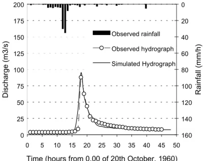
Since the model parameter k was adjusted by using only the observed record of the flood event of October 7th, 1970, the performances of the model in reproducing other observed hydrographs can indicate the reliability of the model and its ability to represent the flood regime of the Bisagno River. The model FEST98 was validated using the records of the 20th October 1960 flood event. The simulated flood event is reported in Fig. 12. The simulated flood hydrograph peak time occurred an hour before the recorded one The peak flow is reproduced with an overstimation of about 7 m3_s–1

on a recorded flood peak of 88 m3_s–1_{. The mean absolute}

relative error and the correlation coefficient are 0.01 and 0.85 respectively. The observed runoff coefficient, 0.50, is close to its simulated counterpart, which is 0.48. Overall, the hydrograph appears to be simulated fairly satisfactorily for the present analysis and the peak flow and time are particularly well reproduced.

Combining the GNSRP and FEST98

models

Monte Carlo simulation runs for 1000 years were performed using the GNSRP(2) and FEST98 models under the current

scenario, that is, using present basin land use (Fig.13) to parameterise the FEST98 model. This yields two long sequences of sub-hourly (15 minutes) synthetic streamflow data that provide a sample for each investigated cross-section of the river network. By repetition of this procedure, a large number of simulations (100) produced composite estimates of annual flood series (AFS) at each site, thus obtaining a composite cumulative distribution function of maximum annual flow. Flood frequency analysis is then performed using the Generalized Extreme Value (GEV) distribution.

Complementary studies of regionalisation (De Michele and Rosso, 2001) of the flood frequency regime in Thyrrhenian Liguria indicate that the Generalized Extreme Value probability distribution is the most appropriate to model extreme flows in the area. The cumulative distribution function of the GEV model is given by

              α ξ − − − = ' / 1 ' ' '₍ ₎ 1 exp ) ( k x k x F ₍₃₎

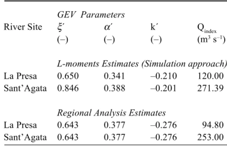
Table 5. L-moment estimates of the GEV distribution parameters and Qindex obtained using the simulated AFS and regional estimates.

GEV Parameters

River Site ξ´ α´ k´ Q_index

(–) (–) (–) (m3_s–1₎

L-moments Estimates (Simulation approach) La Presa 0.650 0.341 –0.210 120.00 Sant’Agata 0.846 0.388 –0.201 271.39

Regional Analysis Estimates

La Presa 0.643 0.377 –0.276 94.80 Sant’Agata 0.643 0.377 –0.276 253.00

Fig. 13. Land use map for the Bisagno river basin.

Table 4. Comparison between observed and simulated hydrograph.

Recorded Simulated Simulated

event [CN2] [CN3]

Peak flood (m3_s–1₎ ₁₁₉ _72.2 ₁₂₇

Peak time (hours) 41 41.50 41.50 Correlation coefficient [R2_] _0.65 _0.80

Mean Error [Mn] 8.98 0.01

Urban area Wood and forest Shrub and bush Grass Special crops Olive Wineyard Crop Bare soil

(15)

where α´ denotes the scale parameter, ξ´ the location parameter and k´ the shape parameter determining the type of asymptotic tail of the probability curve. Accordingly, this distribution was used to estimate flood frequency curves from the simulated AFS. The GEV parameters were estimated using the method of L-moments, as the simplest and most efficient estimator for this distribution (Stedinger et al., 1993), from the grouped AFS. This smooths out sampling fluctuations from Monte Carlo simulation runs on the assumption that both the simulation outcomes and the historical records come from the same parent distribution. Table 5 lists the values of the GEV parameters and the mean annual maximum flow (Q_index) for the two cross-sections mentioned above. Finally, the suitability of the simulation procedure, based on the combination of stochastic and deterministic simulation (S-approach) was assessed by comparing the simulated flood frequency curves with frequency curves determined by the regionalisation (R-approach) and by derived distribution techniques (D-approach)..

As mentioned above, for Thyrrhenian Liguria the GEV probability distribution provides a satisfactory fit to ordered sampling data of re-normalised AFS. The T-year flood, Q_T, is thus given by                       − − + = k index T _T T k Q Q 1 ln 1 ' ' ' α ξ (4)

where ξ´, α´, k´ and Qindex have the same meaning as before.

In the case of the regional approach (R-approach), the values of parameters ξ, α and k, obtained by the method of L-moments and shown in Table 5, are the same for the two cross-sections. The index flood is evaluated as the sampling mean for the gauged La Presa river site. Different methods, used to estimate the index flood for the ungauged site of Sant’Agata, yielded estimates within a range of 15%. Because of the long-term information available from historical and proxy data, the historical flood marks technique was included because it provides the estimate with the lowest variance.

Flood frequency estimation was studied also by the derived distribution approach by the Second Order Second Moment (SOSM) method (Adom et al.,1989). This approach makes use of the geomorphoclimatic information (e.g. mean averaged intensity and mean duration of storm event, climatic factor of scale, basin area, saturation volume per unit area, time lag of basin and mean annual number of independent floods) to evaluate the second order statistics of the candidate probability model, but the parent frequency distribution must be selected “a-priori”. Therefore, the EV1, EV2 and GEV distributions for the AFS are used,

respectively, to investigate the sensitivity of the result to the choice of the parent cumulative density function (CDF) of the partial duration series (PDS). Under the assumption of Poisson occurrence of flood events as a stochastic point process, the exponentially distributed PDS yields the EV1 distributed AFS, the Pareto distributed PDS yields the EV2 distributed AFS, and the Generalized Pareto distributed PDS yields the GEV distributed AFS. Table 6 gives the estimated parameters from the SOSM-EV1 and SOSM-EV2 approaches, where a and b denote the scale and location parameter of the EV1, while x₀> 0 and q > 0 stand for the scale and shape parameter of the EV2.

The parameters of the GEV distribution were also estimated on the assumption that the shape parameter k equals the regional value. Accordingly, the SOSM geomorphoclimatic estimates were used to fit the values of ξ and α. The results are listed in Table 6 for the two cross-sections examined. Therefore, it is assumed that the shape exponent of the GEV equals that of the regional GEV growth curve. Also, the rate of occurrence of the Poisson process must be evaluated from storm data analysis.

The results are reported in Fig. 14 for the La Presa and Sant’Agata river sites, respectively, in the Bisagno river. As expected, the influence of the parent is significant, especially for extreme flows with return period higher than Table 6. EV1- EV2- GEV parameter estimates and index flood obtained using the SOSM method.

SOSM Method Parameters Estimates EV1 Distribution

River Site a b Q_index

(m3_s–1₎ _(m3_s–1₎ _(m3_s–1₎

La Presa 39.6 78.3 101.1

Sant’Agata 108.2 208.9 271.4 EV2 Distribution

River Site θ x_o Q_index

(–) (m3_s–1₎ _(m3_s–1₎

La Presa 2.40 51.90 79.4 Sant’Agata 2.36 135.2 289.8

GEV Distribution

River Site _ξ _α k Q_index

(m3_s–1₎ _(m3_s–1₎ _(–) _(m3_s–1₎

La Presa 63.4 33.3 –0.276 95.0 Sant’Agata 168.2 91.1 –0.276 254.6

(16)

0 100 200 300 400 500 1 10 100

Return period, years

Maximum annual flow, m

3 s

-1 R-approach

D-approach (SOSM GEV) S-approach (Distributed Model) Observed Data Bisagno at La Presa (34.1 Km2) 0 1 2 3 4 5 1 10 100

Growth Factor, x = Q /E[ Q ] R-approach SOSM GEV

S-approach (Distributed Model) Observed Data Bisagno at La Presa (34.1 Km2) 0 250 500 750 1000 1250 1500 1 10 100

3s

-1 R-approach

D-approach (SOSM GEV) S-approach (Distributed Model)

Bisagno at Sant'Agata Bridge (92.1 Km2)

0 1 2 3 4 5 1 10 100

Growth Factor, x = Q /E[ Q ] R-approach

D-approach (SOSM GEV) S-approach (Distributed Model)

0 100 200 300 400 500 1 10 100

3 s

-1

R-approach

D-approach (SOSM GEV) D-approach (SOSM EV1) D-approach (SOSM EV2) Observed Data Bisagno at La Presa (34.1 Km2) 0 250 500 750 1000 1250 1500 1 10 100

3 s

-1

D-approach (SOSM GEV) D-approach (SOSM EV1) D-approach (SOSM EV2) R-approach

Fig. 13. Flood frequency estimates at La Presa (a) and Sant’Agata (b) in the Bisagno river as evaluated from the SOSM D-method where the

parent EV1, EV2 and GEV are used. The sampling mean and the index-flood estimated from flood marks are used for rescaling the regional growth curve at La Presa and Sant’Agata, respectively, in the application of the R-approach.

Fig. 15. Flood frequency estimates at La Presa in the Bisagno river as evaluated from (1) the R-method (Regional GEV plus sampling index

flood), (2) the D-method (SOSM with parent GEV) and (3) the S-method using the FEST98 distributed model. Maximum annual flow vs. return period is shown in plot (a), while the indexed figures are reported in plot (b).

Fig. 16. Flood frequency estimates at Sant’Agata in the Bisagno river as evaluated from (1) the R-method (Regional GEV plus historical marks

index flood), (2) the D-method (SOSM with parent GEV) and (3) the S-method using the FEST98 distributed models. Maximum annual flow vs. return period is shown in plot (a), while the indexed figures are reported in plot (b).

(17)

ten years. This is also reflected by the values of the index-flood (i.e. the mean annual index-flood) reported in Table 6. Therefore, one must select the appropriate parent using the R-approach. To this effect, one notes that the parent GEV distribution provides a satisfactory fit of the observed 48-years data sample for La Presa station, and it is also in good agreement with the regional GEV distribution.

The frequency curves computed by different methods were compared using the data and models developed for the Bisagno River case study. These estimates include those obtained from the application of the R-, D- and S-approaches. The analysis has been performed for the two major river sites of the Bisagno river, that is, the gauged site of La Presa with a catchment area of about 34 km2_{, and}

the ungauged site of Sant’Agata with a catchment area of about 92 km2_{, which is located immediately upstream of}

the culvert tunnelling the river outlet to the Thyrrhenian sea (see Figs. 15 and 16, respectively).

Because the D-approach using SOSM approximation is strongly dependent on the choice of the parent distribution, a parent GEV is adopted here as it results from regionalisation analysis. Accordingly, the regional value of the shape parameter is used to represent the local GEV cumulative density function with location and scale parameters estimated by the SOSM approach. The resulting flood frequency curves are displayed in Figures 14 and 15 for La Presa and Sant’Agata river sites, respectively. The corresponding growth curves are also shown, that is, the indexed flood peak flow against return period. This is to assess the impact of the approach on the shape of the flood frequency curve.

The results indicate that these methods yield close extreme flood estimates. The deviation of various estimates for high flows is definitely confined to the uncertainty band associated with the flood estimates for large return periods, although a number of drawbacks can affect their application in a case study. One also finds that the R-, D- and S-approaches lead to a common probability model, that is, the GEV probability distribution with negative shape parameter, although one notes that the D-approach is forced to assume the same shape parameter of the regional growth curve. The application to a case study with less detailed information than that collected for the Bisagno River case study is obviously subject to larger uncertainties, and the deviations can be more pronounced. The major challenge is to achieve a coherent parameterisation of this probability model using different approaches.

Summary and conclusion

The ability of a combination of stochastic and deterministic

simulations to perform flood frequency analysis of the Bisagno River basin in Northern Italy was assessed. This approach couples the rainfall generation model GNSRP(n), where n stands for the number of raincells, with the rainfall-runoff model FEST98. The calibration of the GNSRP(n) was performed using a continuous record of seven-years hourly precipitation data from five raingauges scattered over the basin surface. Thousand-years’ series of continuous rainfall data were generated for the gauging sites and an extreme-value-oriented method was used for model validation by comparing historical and simulated DDF-curves at different scales of temporal aggregation. The synthetic precipitation series were then used as inputs to FEST98 model, which provided 15-minutes streamflow data for two selected cross-sections of the river network. These data were then processed to obtain the AFS at the two river sites. Flood frequency analysis of the AFS retrieved from the simulation runs was carried out using the GEV distribution with parameters estimated through the method of L-moments. Flood frequency curves of simulated data were then compared with frequency curves determined by application of the regionalisation and the derived distribution techniques.

A more comprehensive comparison between estimation methods focused on the predictive capabilities of the different methods in respect of the index flood and of a number of quantiles traditionally used in hydrological practice. Specifically: (a) the predictive capability of simulation techniques in relation to the index flood, dependent upon the adequacy of suitable stochastic rainfall and rainfall-runoff models, is considerably higher than that of statistical and/or physically based regionalisation or that of methods based on or derived from distribution techniques; (b) the joint use of generated rainfall and rainfall-runoff simulation models can provide a robust estimate of the index flood for ungauged catchments (the more explicit the parameterisation is in respect of available data, the larger is the transferability of the model from catchment to catchment); however, uncertainty remains both in the structure of the model and in estimation of its parameters.

The present state of the art of flood estimation techniques is still characterised by uncertainties, which cannot be overcome by any single approach. The combined use of flood estimation methods that use simulation techniques to estimate the index flood and of the regional parent distribution to estimate the quantiles seems to be a reasonable compromise. The great potential offered by the Monte Carlo approach to estimate the rarest events seems to be limited by some inaccuracies in the rainfall generator, which should be further tested with respect to the representativeness of the temporal patterns of generated

(18)

storm events. Because the historical data set used for GNSRP calibration comprised only seven years of data, the GNSRP model may require a large amount of rainfall data to obtain a better calibration and validation in terms of DDF. On the other hand, the FEST98 model requires an adequate parameterisation of the soil and channel network that necessitates detailed knowledge of the catchment. The methodology developed appears specially useful to predict low-frequency discharge in catchments where long series of rainfall records are available and a detailed catchment survey can be conducted but, as occurs frequently in hydrology, flow discharge has seldom been recorded over a long period.

Acknowledgements

The research was supported jointly by the European Commission through grant ENV4-CT97-0529 (FRAMEWORK project) and by CNR GNDCI of Italy through grant n. 01.01072.PF42. Grateful thanks are due to Enda O’Connell and Aidan Burton (University of Newcastle upon Tyne, England, UK) for rainfall modelling facilities. The Hydrographic Service of Genoa is acknowledged for providing hourly rainfall data in the study area.

References

Adom, D.N., Bacchi, B., Brath, A. and Rosso, R., 1989. On the geomorphoclimatic derivation of flood frequency (peak and volume) at the basin and regional scale, in: New Directions for

Surface Water Modelling, M.L. Kavvas, Ed. IAHS Publ. no. 181, 165–176.

Band, L.E., 1986. Topographic partition of watersheds with digital elevation models. Water Resour. Res., 22, 15–24.

Brath, A. and Montanari, A., In press. The effects of the spatial variability of soil infiltration capacity in distributed flood modelling. Hydrol.Process.

Burlando, P. and Rosso, R., 1991. Comment on “Parameter estimation and sensitivity analysis for the modified Bartlett-Lewis rectangular pulses model of rainfall” by S. Islam et al.

J. Geophys. Res., 96, 9391–9395.

Burlando, P. and Rosso, R., 1996. Scaling and multiscaling models of depth-duration-frequency curves of storm precipitation.

J.Hydrol., 187, 45–64.

Cameron, D.S., Beven, K.J., Tawn, J., Blazkova, S. and Naden, P., 1999. Flood frequency estimation for a gauged upland catchment (with uncertainty). J Hydrol., 219, 169–187. Cameron, D.S., Beven K.J. and Tawn, J., 2000. An evaluation of

three stochastic models. J. Hydrol., 228, 130–149.

Cowpertwait, P.S.P., 1994. A generalized point process model for rainfall. Proc. Roy. Soc. Lond., A 447, 23–37.

Cowpertwait, P.S.P., 1995. A generalized spatial-temporal model of rainfall based on a clustered point process. Proc. Roy. Soc.

Lond., A 450, 163–175.

Cunge, J,A., 1969. On the subject of a flood propagation computation method (Muskingum Method). J. Hydraul. Res. 7, 205–230.

De Michele, C., Montanari, A. and Rosso, R., 1998. The effects of non-stationarity on the evaluation of critical design storms,

Water Sci. Technol., 37, 187–193.

De Michele, C. and Rosso, R., 2001. A Multi-level approach to flood frequency regionalization. In: Proc. 21st Ann. Amer. Geophys. Un. “Hydrology Days”, J. A. Ramirez (Ed.) Colorado State University, Fort Collins, Colorado. 264–277.

Kuntner, R. and Burlando, P., 2000. Characterising the effects of landuse and climate changes on rainfall excess in alpine and prealpine catchments using a landuse-oriented model (Abstract), European Conference on Advances in Flood Research, Potsdam, November 1-3, 2000.

La Barbera, P., Risso P.P. and Siccardi F.,1978. L’idrologia di superficie del T. Bisagno. Determinazione degli input idrologici con associato periodo di ritorno per il calcolo delle portate temibili in diverse sezioni di chiusura, Atti del Seminario su

Estremi Idrologici e Modelli di Previsione, CNR-IRPI, Perugia.

Leopold, L.B. and Maddock, T., 1953. The hydraulic geometry of stream channels and some physiographic implications. Prof. Pap. 252, U.S. Geol. Survey, Washington, D.C.

Mancini, M., 1990. Modelling catchment hydrologic response:

effects of the spatial variability and the scale of representation of the soil absorption phenomenon. Ph.D. Thesis (in Italian),

Politecnico di Milano, Milan. 156 pp.

Mancini, M., Montaldo, N. and Rosso, R., 2002. La modellistica distributa nella valutazione degli effecti di laminazione do un sistema di invasi artifialli nel bacino del fiume Toce. L’Acqua, 4, 31–42.

Mark, M.D., 1983. Automated detection of drainage network from digital elevation models. Auto-Carto, 6, 169–178.

Montgomery, D.L. and Foufoula-Georgiou, E., 1993. Channel network source representation using digital elevation models.

Water Resour. Res., 29, 3925–3934.

Onof, C. and Wheater, H.S., 1993. Modelling of British rainfall using a random parameter Bartlett-Lewis rectangular pulse model. J.Hydrol., 149, 67–95.

Orlandini, S. and Rosso, R., 1998. Parameterization of stream channel geometry in the distributed modeling of catchment dynamics. Water Resour. Res., 103, 1971–1986.

Ponce, V.M., 1989. Engineering Hydrology. Prentice Hall, NJ. Rodriguez-Iturbe, I., Cox, D.R. and Isham, V., 1987. Some models

for rainfall based on stochastic point processes. Proc. Roy. Soc.

Lond. A 410, 269–288.

Rosso, R. and Rulli, M.C., 2002. An integrated simulation method for flash-flood risk assessment: 1. Effects of historical land use changes. Hydrol.Earth Syst. Sci., 6, 285–294.

Soil Conservation Service, 1972. National Engineering Handbook,

section 4, Hydrology. US Dept. of Agriculture: Washington D.C.

Sorooshian, S., 1983. Surface water hydrology: on-line estimation.

Rev.Geophys. Space Phys. 31, 706–721.

Stedinger, J.R., Vogel, R.M. and Foufoula-Georgiou, E., 1993. Frequency analysis of extreme events, chapter 18. In: Handbook

(19)