_____________________________________________________________________________________________________ *Corresponding author: E-mail: jean-beguinot@orange.fr;
Numerical Extrapolation of the Species Abundance
Distribution Unveils the True Species Richness and
the Hierarchical Structuring of a Partially Sampled
Marine Gastropod Community in the Andaman
Islands (India)
Jean Béguinot
1*1
Department of Biogéosciences, UMR 6282, CNRS, Université Bourgogne Franche-Comté, 6, Boulevard Gabriel, 21000 Dijon, France. Author’s contribution The sole author designed, analyzed, interpreted and prepared the manuscript.
Article Information
DOI: 10.9734/AJEE/2018/41293 Editor(s): (1)Wen-Cheng Liu, Professor, Department of Civil and Disaster Prevention Engineering, Taiwan Typhoon and Flood Research Institute, National United University, Taiwan.
Reviewers: (1)Manoel Fernando Demétrio, Universidade Federal da Grande Dourados, Brazil. (2)Komal Bangotra, University of Jammu, India. Complete Peer review History:http://www.sciencedomain.org/review-history/24491
Received 27th February 2018 Accepted 1st May 2018 Published 7th May 2018
ABSTRACT
Even when it remains substantially incomplete, the partial inventory of a species assemblage can provide much more information than could be expected at first. This can be achieved by applying a rigorous numerical extrapolation procedure that fully extends the incomplete sampling in numerical terms and, thereby, provides reliable estimates regarding not only the number but also the distribution of abundances for the whole set of the undetected species. As a result, this makes available the full range of the Species Abundance Distribution of the yet partially sampled assemblage and, thus, allows to address a series of interesting issues regarding the process and pattern of the hierarchical structuring of species abundances within the studied assemblage of species. Moreover, the same kind of numerical extrapolation may be applied separately to each subset of species, within the whole assemblage, that may have relevant interest (taxonomic subgroups, feeding guilds, etc…). Thus, deconstructing the Species Abundance Distribution can provide further detailed insights into the functional organisation of the studied assemblage.
The mathematical and algorithmic basis for this extrapolating procedure has been developed recently, to be applied to the numerical extension of both the Species Accumulation Curve and the Species Abundance Distribution.
The wide potential interest of this new methodological approach, when having to deal with substantially incomplete inventories of species (which is doomed to become inevitable with increasingly species-rich assemblages), is illustrated by a detailed case study of a marine gastropod assemblage on rocky shore under tropical climate.
Keywords: Species richness; diversity; rank-abundance; marine snails; trophic rank; least-biased estimation; incomplete sampling.
1. INTRODUCTION
Total species richness, taxonomic composition
and hierarchical structuring of species
abundances are three key features that appropriately characterise species communities. Unfortunately, partial, incomplete inventories – which are doomed to become even more frequent with the inevitable generalisation of “rapid assessments” and “quick surveys” – prevent an in-depth appreciation of each of these key aspects of species communities [1–3]. However, a properly implemented procedure of
numerical extrapolation can provide reliable
estimations relative to both the number and the respective abundances of the undetected species and, thereby, allows the derivation of reliable inferences as regard (i) the true, total species richness and (ii) the distribution of species abundances completed by including the subset of still undetected species. Only the taxonomic identities of the latter inevitably escape to any attempt of extrapolation. In turn, once numerically completed (and only when it is so: [4]), the distribution of species abundances can provide some synthetic pieces of information about the process at work (either deterministic or stochastic) that drive the hierarchical structuring of species abundances within the community [5– 9]. Although no further mechanistic details may be extracted from this synthetic overview, it has, yet, the advantage of being straightforward, as it does not require the long and tedious analytical approaches that would be required otherwise to go deeper in the details of structuring processes. As such, this synthetic approach can serve as a convenient preliminary approach.
As complete abundance distributions (or, if not the case, their completed version using
numerical extrapolation) are mandatory, a
procedure for the numerical extrapolation of the Species Accumulation Curve and the Species Abundance Distribution (the former directly linked to the latter) has recently been developed,
aiming at providing reliable, least-biased
inferences about the number and the respective abundances of undetected species, when having to deal with substantially incomplete inventories. Tropical marine ecosystems in shallow waters are of major interest to ecologists and conservationists, as they are considered as embodying remarkably high levels of biological complexity among marine communities [10–12]. However, and precisely because of their usually high species richness and diversity (including
numerous rare species), samplings of these
communities often remain substantially
incomplete [4]. For all the reasons just mentioned above, such partial inventories thus require implementing reliable numerical extrapolation procedure, so as to release as much information as possible regarding (i) the true species richness of sampled community, (ii) a synthetic overview of the hierarchical structuring of species abundances and (iii) how specific are the respective functional contributions of the different trophic levels involved in the community.
Hereafter, I report and discuss the results derived from the numerical extrapolation of a partial inventory of an intertidal gastropod community established on a rocky shore near Rangat, Andaman Islands, India [12].
2. MATERIALS AND METHODS 2.1 Materials
The rocky shore of Andaman and Nicobar Islands is home to a rich fauna of marine gastropods [13]. Yet, detailed inventories of gastropod communities at the local scale, including species abundances, remain very
scarce. A recent report by JEEVA et al. [12]
opportunely provides such a series of local inventories along the rocky shores of Andaman Islands. But, referring to the high proportion of singletons (species that were detected only once
during sampling), these inventories remain substantially incomplete [14–16]. Accordingly, implementing numerical extrapolation
inventories is required to uncover the series of useful information that may be derived from complete (here completed by extrapolation Species Abundance Distributions, as mentioned above.
Hereafter, I shall focus on the particular community that provides the highest number of recorded species; this community is located near Rangat, in the southern part of Middle Andaman.
According to JEEVA et al. [12]. The sampled area
is mainly covered by rocky outcrops with boulders and pebbles and the partial inventory was conducted by these authors at the intertidal level.
2.2 Numerical Extrapolation Procedures * Total species richness: the least
estimation of the number of still undetected species during partial sampling and the resulting least-biased estimation of the total species richness of the sampled community are derived according to the procedure defined by Béguinot [17,18] and briefly summarised in Appendi
basis of the numbers fx
observed x-times during partial sampling, as provided in Appendix 3).
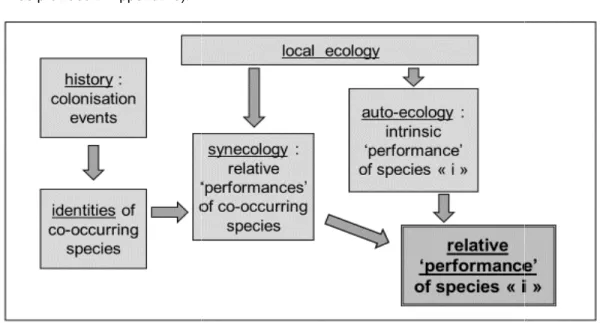
Fig. 1. Schematic sketch showing how the combination of both historical and ecological contexts peculiar to a given community of species drive the relative
- sensu latissimo - of each member
of species abundances in the community
during sampling), these inventories remain 16]. Accordingly,
numerical extrapolation of such
inventories is required to uncover the series of useful information that may be derived from
completed by extrapolation)
Distributions, as mentioned
Hereafter, I shall focus on the particular community that provides the highest number of recorded species; this community is located near Rangat, in the southern part of Middle Andaman. e sampled area is mainly covered by rocky outcrops with boulders and pebbles and the partial inventory was conducted by these authors at the intertidal
Extrapolation Procedures : the least-biased number of still undetected species during partial sampling and the biased estimation of the total species richness of the sampled community are derived according to the procedure defined by Béguinot [17,18] and briefly summarised in Appendix 1, on the of species times during partial sampling,
* Species Abundance Distribution
accurately exploit their full potential, the
as-recorded Species Abundance
Distributions (“S.A.D.s”) require [19,20]:
- First, to be corrected
sampling bias, resulting from the finite size of samplings and,
- Second, but still more importantly, to be
completed by numerical extrapolation to
the extent that sampling is suspected to be incomplete, as revealed by the subsistence of singletons.
The appropriate procedure of numerical extrapolation and correction of
recorded S.A.D.s - described in
in Béguinot [20] - is briefly recalled in Appendix 2.
After being corrected and
accordingly, the S.A.D.: (i) not only provides an overview of both the true species richness of the sampled community and the diversity of the respective abundances of member species also, (ii) can help addressing several important questions regarding the kind of process driving the hierarchical structuration of the community, including possible specificities according to th different trophic levels involved in the community of interest (Fig. 1).
Schematic sketch showing how the combination of both historical and ecological contexts peculiar to a given community of species drive the relative “performance”
of each member species "i", thus generating the hierarchical structuring of species abundances in the community
Species Abundance Distribution: to accurately exploit their full potential, the
recorded Species Abundance
require [19,20]: for statistical sampling bias, resulting from the finite , but still more importantly, to be by numerical extrapolation to the extent that sampling is suspected to be incomplete, as revealed by the
The appropriate procedure of least-biased numerical extrapolation and correction of the
as-described in details
is briefly recalled in
and extrapolated
only provides an overview of both the true species richness of the diversity of the respective abundances of member species, but can help addressing several important questions regarding the kind of process driving the hierarchical structuration of the community, including possible specificities according to the different trophic levels involved in the community
Schematic sketch showing how the combination of both historical and ecological “performance” hierarchical structuring
More precisely, these questions may relate to:
- The process of structuration of a community of species: for example, does only one (or very few) dominant factor is (are) at work to structure the community or, on the contrary, do many independent factors are contributing together; which may be tested by checking the conformity of the corresponding S.A.D. to either the
log-series model or the log-normal model
respectively [5,21–24];
- The degree of structuration of a community
of species, which broadly refers to the level
of unevenness between species
abundances within the community. This may be appropriately tested by comparing the slope of the corresponding S.A.D. to either the “ideally even” model or the “broken-stick” model [20]. These two models provide two reference levels of structuration, namely the “ideally even” model characterises the zero level of
structuration, while the “broken-stick”
model accounts for the degree of structuration that would be obtained by a
random apportionment of relative
abundances among all co-occurring
species in the community. Thus
standardising the degree of structuration (the slope of the S.A.D.) with respect to the “broken-stick” model is particularly relevant as this allows to leave aside the “mechanistic”, trivial influence of the number of member species and, thus, to account only for the genuine hierarchical structuring [7,8,25]. Thus standardised, the degree of structuration of the community becomes independent of its richness in species. This “mechanistic” influence of the level of species richness on the degree of community structuration, that is on the
slope of the abundance distribution, is demonstrated in Appendix 3.
3. RESULTS
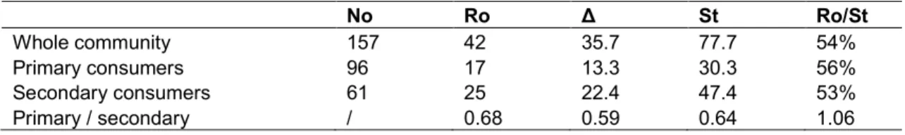
3.1 Estimation of the Total Species Richness of the Community as a Whole and Separately by Kind of Feeding Guild
Accounting for the values of the numbers fx of
species observed x-times during partial sampling (Fig. A1 in Appendix 1), the least-biased nonparametric estimator of the number of
undetected species during the partial
sampling proves to be Jackknife-5 (see the selective key in Appendix 1). The corresponding least-biased estimations of (i) the number Δ of
undetected species, (ii) the resulting level St of
the total species richness of the sampled community and (iii) the level of completeness, Ro/St of the incomplete sampling are provided in Table 1. With a 54% level of completeness only, the partial sampling confirms remaining very far from exhaustivity.
The separate estimations of Δ and St, according
to feeding guilds – primary and secondary consumers respectively – are subsequently derived. Similar levels of sampling completeness are inferred for both guilds (56% and 53% respectively).
Due to the relatively low level of achieved sampling completeness, further sampling could be considered of interest. In this perspective, the
least-biased extrapolation of the Species
Accumulation Curve highlights the expected increase in the number of detected species, R(N), as a function of growing sampling size N, beyond the actually achieved inventory. And, thereby, the additional sampling efforts that would be required to obtain any desirable increase in sampling completeness can be forecasted, as shown in Fig. 2.
Table 1. Numerical characteristics of a marine Gastropod community at the intertidal level of a rocky shore at Rangat (Andaman Islands), including: the sampling-size No, the number of detected species Ro (= R(No)), the estimated number of undetected species Δ, the resulting
evaluation of total species richness St and the level of sampling completeness Ro/St No Ro Δ St Ro/St Whole community 157 42 35.7 77.7 54% Primary consumers 96 17 13.3 30.3 56% Secondary consumers 61 25 22.4 47.4 53% Primary / secondary / 0.68 0.59 0.64 1.06
Fig. 2. Extrapolated part of the Species Accumulation Curve accounting for the increase of the number of detected species R(N) as a function of growing sample size N beyond the actually
achieved sampling (No = 157, R(No) = 42). Here, the selected, least-biased, nonparametric estimator of the number of undetected species is Jackknife-5, leading to a total species richness St = 78, with the associated least-biased extrapolation plotted as the coarse solid line. Also plotted for comparison are the extrapolations of the S.A.C. associated to the other,
more biased estimators. In practice, the least-biased extrapolation (coarse solid line) highlights the expected additional sampling effort required to reach improved levels of sampling completeness (for example, the sample sizes required to reach 80%, 90% and 95%
completeness would be around N = 600, 1400, 2900 respectively)
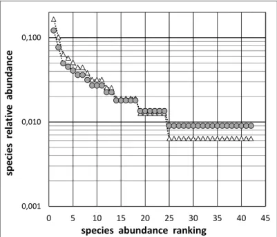
3.2 Correction and Extrapolation of the Species Abundance Distribution The as-recorded part of the Species Abundance Distribution (i.e. the part restricted to the set of actually detected species only) needs being corrected, as shown in Fig. 3. Corrections, made according to equation (A2.1) in Appendix 2, involve both: (i) a positive correction due to the
multiplicative factor (1+1/ni) being >1 and (ii) a
negative correction due to the multiplicative
factor (1–f1/N0)/(1+R0/N0) being < 1. The positive
correction, decreasing progressively with
increasing species abundances, outweighs the negative correction only for the lower species abundances, that is along the second part of the recorded Species Abundance Distribution (here for species ranks i = 19 to i = 42, as highlighted in Fig. 3).
The least-biased extrapolation of the Species Abundance Distribution, from rank 43 to rank 78, is computed according to equation (A2.3) in Appendix 2 and is plotted as the solid line in Fig.
4. This figures thus unveils the entire
development of the Species Abundance
Distribution, duly corrected for its recorded part and extrapolated with minimized bias for the whole set of the still undetected species. Note that, although most undetected species are expected to be among the less abundant in the community, their ecological importance is no less and, thus, deserve as much attention, as already emphasised by several authors [26–28].
The same procedure of correction and
extrapolation is, then, conducted separately for
primary and for secondary consumers, as shown
in Figs. 5 and 6. The superposition of the Species Abundance Distributions for each guild in Fig. 7 allows an easy, direct comparison of the degrees of structuration of species abundances in each guild. An alternative comparative approach is provided in Figs. 8 and 9, in the form of a common histogram of species abundances for the two guilds together. In these Figs, the abundances are plotted on an arithmetic scale, rather than the usual log-transformed scale, in order to offer a direct visual appreciation of the respective contributions of the member species of each guild. As shown in Figs. 7 and 8, the dominant species in term of number of 40 45 50 55 60 65 70 75 0 500 1000 1500 2000 2500 3000 nu mb er of spe cies R(N) sample size N S.A.C. assoc. JK-5 S.A.C. assoc. JK-4 S.A.C. assoc. JK-3 S.A.C. assoc. JK-2 S.A.C. assoc. JK-1 S.A.C. assoc. Chao 54 %(actual sampling completness)
80%
95% 90%
individuals, are predominantly primary
consumers: the four numerically dominant species all belong to the herbivorous family Neritidae: Nerita albicilla Linnaeus 1758, Nerita
polita Linnaeus 1758, Nerita insculpta Récluz
1841, Nerita costata Gmelin 1791 (with corrected
relative abundances: a1 = 0.122, a2 = 0.077, a3 =
0.049, a4 = 0.045, respectively).
Fig. 3. The as-recorded part of the Species Abundance Distribution (white triangles) and the same after correction (grey discs): see text for further explanation
Fig. 4. The completed Species Abundance Distribution, including both
(i) The correction of the recorded part (involving the 42 detected species: grey discs) and (ii) The least-biased extrapolation of the unrecorded part
(i.e. the 36 undetected species: ranks i = 43 to 78: solid line)
0,001 0,010 0,100 0 5 10 15 20 25 30 35 40 45 sp ecie s re la tiv e abund ance
species abundance ranking
0,0001 0,0010 0,0100 0,1000 0 5 10 15 20 25 30 35 40 45 50 55 60 65 70 75 80 species rela tive ab undan ce
Fig. 5. The completed Species Abundance Distribution (corrected: grey discs ; extrapolated: solid line) considering the guild of primary consumers (“herbivores”)
Fig. 6. The completed Species Abundance Distribution (corrected: grey discs; extrapolated: solid line) considering the guild of secondary consumers (“carnivores, scavengers,…”)
0,0001 0,0010 0,0100 0,1000 0 2 4 6 8 10 12 14 16 18 20 22 24 26 28 30 32
sp
ec
ies
r
el
at
iv
e
ab
un
dan
ce
species abundance ranking
primary consumers 0,0001 0,0010 0,0100 0,1000 0 5 10 15 20 25 30 35 40 45
sp
e
ci
e
s
re
lat
ive
a
b
u
n
d
a
n
ce
species abundance ranking
Fig. 7. Superposition of the completed Species Abundance Distributions for primary and secondary consumers (plotted in Figs. 5 and 6), thus allowing direct comparison between both
feeding guilds
Fig. 8. The Species Abundance Distribution for the 42 already detected species, highlighting the feeding mode of each species. Note the arithmetic (instead of
log-transformed) scale for abundances. Directly derived from Figs. 5 & 6
0,0001 0,0010 0,0100 0,1000
0
5
10
15
20
25
30
35
40
45
sp
ec
ies
rela
ti
ve
a
bun
dance
species abundance ranking
0,00 0,02 0,04 0,06 0,08 0,10 0,12 1 3 5 7 9 11 13 15 17 19 21 23 25 27 29 31 33 35 37 39 41
spec
ies
r
ela
tive
a
bu
nd
anc
e
species abundance rank
Titre du graphiqueprimary consumers
secondary consumers
Fig. 9. The Species Abundance Distribution extrapolated for the 35 still undetected species, highlighting the feeding mode of each species. Note the arithmetic (instead of
log-transformed) scale for abundances. Directly derived from Figs. 5 & 6
3.3 Quantitative Characterisation of the Hierarchical Structuring of Species
Abundances in the Studied
Community
3.3.1 The type of structuring process
In order to investigate which kind of structuring process is at work in the studied community, two models of abundance distribution – the
“log-normal” distribution and the “log-series”
distribution – were tentatively fitted to the
completed Species Abundance Distribution
provided at Fig. 4. As shown in Figs. 10 and 11, a fairly good fit is obtained with the log-normal model, while the accordance with log-series is comparatively less satisfactory. The same holds true for both feeding guilds, primary and secondary consumers, considered separately: Figs. 12, 13, 14, 15.
Fig. 10. Two classical models: “log-normal” (coarse dotted line) and “log-series” (double line) fitted to the Species Abundance Distribution of the whole community (corrected and
extrapolated cf. Fig. 4). The best fit is clearly with the "log-normal" distribution
0,000 0,001 0,002 0,003 0,004 0,005 0,006 0,007 43 45 47 49 51 53 55 57 59 61 63 65 67 69 71 73 75 77 sp ec ie s r el at iv e a b u n d an ce
species abundance rank
Titre du graphique primary consumers secondary consumers 0,0001 0,0010 0,0100 0,1000 0 5 10 15 20 25 30 35 40 45 50 55 60 65 70 75 80 spe ci es relativ e ab u nd ance
Fig. 11. The “log-normal” model (coarse dotted line) fitted to the Species Abundance Distribution (as in Fig. 10). Note the arithmetic scale for abundances (instead of log-transformed scale), which allows a more direct visual appreciation of relative abundances,
as suggested by MacArthur [29]
Fig. 12. The “log-normal” model (coarse dotted line) fitted to the Species Abundance
Distribution for the guild of primary consumers
0,00 0,02 0,04 0,06 0,08 0,10 0,12 0,14 0 5 10 15 20 25 30 35 40 45 50 55 60 65 70 75 80
sp
eci
es
rela
ti
ve
abun
danc
e
species abundance ranking
whole community 0,0001 0,0010 0,0100 0,1000 0 2 4 6 8 10 12 14 16 18 20 22 24 26 28 30 32
spe
cie
s
r
e
la
ti
ve
a
bu
nd
anc
e
species abundance ranking
Fig. 13. Same as Fig. 12 but with arithmetic scale for abundances (instead of log-transformed scale), which allows a more direct visual appreciation of relative abundances,
as suggested by MacArthur [29]
Fig. 14. The “log-normal” model (coarse dotted line) fitted to the Species Abundance
Distribution for the guild of secondary consumers
0,00 0,02 0,04 0,06 0,08 0,10 0,12 0,14
0 2 4 6 8 10 12 14 16 18 20 22 24 26 28 30 32
sp
ecie
s
re
la
ti
ve
ab
undan
ce
species abundance ranking
primary consumers
0,0001 0,0010 0,0100 0,10000
5
10
15
20
25
30
35
40
45
sp
ec
ies
r
e
la
tiv
e
abund
ance
species abundance ranking
Fig. 15. Same as Fig. 14 but with arithmetic scale for abundances (instead of log-transformed scale), which allows a more direct visual appreciation of relative abundances,
as suggested by MacArthur [29] 3.3.2 The intensity of the structuring process
The shape of the Species Abundance
Distribution characterises in details the intensity of the hierarchical structuring of species abundances in the community.
As emphasised in the Methods section, in order to unveil the genuine intensity of the structuring process (leaving aside the trivial contribution of the level of species richness), the slope of the Species Abundance Distribution should
preferably be standardised to the slope of the
corresponding "broken-stick" distribution
(corresponding meaning that the "broken-stick" is computed for the same species richness). Accordingly, in Figs. 16, 17, 18, the completed (corrected and extrapolated) Species Abundance
Distribution is plotted together with the
corresponding “broken-stick” distribution.
Comparing the slopes on the same graph thus provides a reliable appreciation of the degree of hierarchical structuring of species abundances.
Fig. 16. The Species Abundance Distribution of the whole community plotted together with the corresponding “broken-stick” distribution (dashed line)
0,00 0,01 0,02 0,03 0,04 0,05 0,06 0 5 10 15 20 25 30 35 40 45 sp ecies r el ative abundan ce
species abundance ranking
secondary consumers 0,0001 0,0010 0,0100 0,1000 0 10 20 30 40 50 60 70 80 sp ec ies r elat ive abun dance
Fig. 17. The Species Abundance Distribution for the guild of primary consumers plotted together with the corresponding “broken-stick” distribution (dashed line)
Fig. 18. The Species Abundance Distribution for the guild of secondary consumers plotted together with the corresponding “broken-stick” distribution (dashed line)
In a more concise, but reductionist approach, the
average slope of the Species Abundance
Distribution provides a convenient appreciation of
the degree of hierarchical structuring.
Accordingly, a “structuring index” (i) highlighting the degree of structuring and (ii) standardised to the corresponding “broken-stick” distribution (for the aforementioned reason), can be defined as the ratio between the average slope of the actual abundance distribution and the average slope of the corresponding “broken-stick” model, with
abundances being classically log-transformed. Thus defined, the structuring index is equal to:
Istr = log(a1/aSt)/log(a’1/a’St)
where a1 and aSt stand for the highest and the
lowest abundances in the studied assemblage
and a’1 and a’St stand for the highest and the
lowest abundances in the corresponding
“broken-stick” distribution having the same
species richness St. Results are given in Table 2.
0,0001 0,0010 0,0100 0,1000 0 2 4 6 8 10 12 14 16 18 20 22 24 26 28 30 32 sp e ci e s r e la tiv e a b u n d a n ce
species abundance ranking
primary consumers 0,0001 0,0010 0,0100 0,1000 0 5 10 15 20 25 30 35 40 45 sp e ci e s r e la tiv e a b u n d a n ce
species abundance ranking
Table 2. The degree of hierarchical structuration (unevenness) of species abundances, quantified as the average slope of the Species Abundance Distribution standardised to the
average slope of the corresponding “broken-stick” distribution (see Figs. 16, 17, 18)
Sp. Abund. Distr. “broken-stick” structuring index
log[a1/aSt] / log[a’1/a’St] a1 aSt a'1 a'St Whole community 0.122 0.00016 0.0640 0.00017 1.12 Primary consumers 0.122 0.00019 0.0725 0.00060 1.35 Secondary consumers 0.085 0.00035 0.0451 0.00022 1.03
Fig. 19. Body-size versus relative abundance relationship for the 42 sampled species in the whole community. Relative abundances corrected according to equation (A2.1)
Fig. 20. Body-size versus relative abundance relationship for the 17 sampled species of the guild of primary consumers. Relative abundances corrected according to equation (A2.1)
0 10 20 30 40 50 60 70 80 90 100 0,00 0,02 0,04 0,06 0,08 0,10 0,12 0,14
com
mon b
o
d
y
siz
e
(mm
)
species relative abundance a
iwhole community 0 10 20 30 40 50 60 70 80 90 100 0,00 0,02 0,04 0,06 0,08 0,10 0,12 0,14
co
m
mo
n
b
o
dy siz
e (
m
m)
species relative abundance a
iFig. 21. Body-size versus relative abundance relationship for the 25 sampled species of the guild of secondary consumers. Relative abundances corrected according to equation (A2.1)
3.3.3 Body-size versus relative abundance relationships
Figs. 19, 20, 21 highlight the relationships between the shell-size – as a surrogate to body-size – and the corresponding relative abundance of each actually sampled species (of course, numerical extrapolation provides no information on body-size of undetected species).
Primary and secondary consumers differ
regarding their respective ranges of shell-size (Figs. 20 and 21). Considering an arbitrarily fixed threshold-size of 40 mm:
- Only one species (out of 17) has a
common-size in excess of 40 mm among
primary consumers;
- Eleven species (out of 25) have a
common-size in excess of 40 mm among
secondary consumers.
The difference in proportions (6% against 44%)
is statistically significant:χ2 with Yates correction
= 6.8, p < 0.01. The largest species among
secondary consumers are: Harpa major Röding
1798 (≈ 95 mm), Vasum turbinellus (Linnaeus 1758) (≈ 85 mm), Chicoreus brunneus (Link 1807) (≈ 75 mm), Semicassis bisulcata (Schubert & Wagner 1829) (≈ 55 mm), Bufonaria echinata
(Link 1807) (≈ 50 mm), Latirolagena
smaragdulus (Linnaeus 1758) (≈ 50 mm), Gemmula vagata (E.A. Smith 1895) (≈ 50 mm), Bursa granularis (Röding 1798) (≈ 48 mm), Tylothais virgata (Dillwyin 1817) (≈ 45 mm), Pollia undosa (Linnaeus 1758) (≈ 45 mm),
Polinices mammilla (Linnaeus 1758) (≈ 45 mm).
The largest species among primary consumers is: Scutellastra flexuosa (Quoy & Gaimard 1834) (≈ 70 mm).
4. DISCUSSION
A thorough approach to the species diversity and the hierarchical structuring of abundances in species assemblages would arguably require (quasi-) exhaustive samplings. Yet, incomplete samplings usually become unavoidable practice as soon as species-rich assemblages are
addressed, especially when dealing with
invertebrate’s communities. Hopefully, the
implementation of appropriate extrapolating methods can “force” incomplete samplings and
partial inventories to reveal much more
information than one might think a priori. Thus,
proper numerical extrapolations of both the Species Accumulation Curve and the Species Abundance Distribution provide an unexpected set of additional information relative to all those species that remained undetected after partial samplings. This, in turn, allows to tackle the main issues relative to (i) the evaluation of species richness and (ii) the highlighting of internal
organisation within partially sampled
communities – all subjects that would normally require an exhaustive species inventory.
A thorough analysis of the intertidal gastropod community on the rocky shore at Rangat location
(Andaman Islands) was conducted
accordingly, in compliance with this
methodological approach. 0 10 20 30 40 50 60 70 80 90 100 0,00 0,02 0,04 0,06 0,08 0,10 0,12 0,14 com mon b od y siz e (m m)
species relative abundance ai
4.1 Total Species Richness Estimates
and the Forecasted Additional
Sampling Efforts Required to
Improve Sampling Completeness At first, the estimator Jackknife at order 5 reveals being the least-biased one among the series of classical nonparametric estimators of the number of undetected species (according to the selective key in Appendix 1). This selection of Jackknife-5 proves satisfying, here, not only for the community as a whole but also for each of the two feeding guilds considered separately. The estimated true species richness reaches 77 species for the whole community, among which 30 primary-consumers and 47
secondary-consumers (Table 1), which substantially
exceeds the corresponding recorded numbers (42, 17, 25 species respectively). Thus, the sampling-completeness levels reached for the whole community as well as for the sub-inventories of the two feeding guilds all hardly exceed 50%. This justifies, a posteriori, the need
of implementing an accurate numerical
extrapolation of the partial inventory of this marine gastropod community.
As a comparison, the total species richness of marine gastropods assemblages on coral reefs around each of three small islands in Mannar Gulf (India) was estimated from 49 to 53 species only [30].
Although these extrapolations will provide a lot of additional interesting information regarding the set of still unrecorded species (as described below), further field investigation effort, aiming at increasing the completeness of inventory, might nevertheless be considered. If so, a reliable forecast of the additional sampling effort required to meet a given target gain in sampling-completeness would be useful for the optimal planning of required resources and efforts. The
least-biased extrapolation of the Species
Accumulation Curve associated to the least-biased estimator (here Jackknife-5) answers appropriately this demand, as shown in Fig. 2. Clearly, any further improvement of sampling completeness rapidly requires strong additional investment of sampling effort. Thus, increasing completeness from the actual 54% level to 80% or 90% would require multiplying the actual sample-size by four or by ten respectively. Being able to reliably estimate the level of such additional efforts is of obvious prime interest to rationally decide whether to continue sampling
operation any further or to rely only on the actual inventory as such but adequately extended by numerical extrapolation.
4.2 Correction and Extrapolation of the Species Abundance Distribution The as-recorded distribution needs correction and extrapolation because it is both (i) slightly
biased, due in particular to sampling stochasticity
and, most importantly, (ii) incomplete to the extent of the proportion of those species of the sampled community that remained undetected during sampling.
The corrections, computed according to equation (A2.1), involve (i) a negative contribution
(multiplying factor (1–f1/N0)/(1+R0/N0) which is <
1) related to the degree of sampling
incompleteness and (ii) a positive contribution
(multiplying factor (1+1/ni) which is >1) that
compensates for statistical bias during sampling [20]. These combined corrections result in a slight reduction of higher abundances and a slight increase of lower abundances, as shown in Fig. 3.
In turn, the numerical, least-biased extrapolation of the distribution of abundances provides the
complete development of the Species
Abundance Distribution, as would be obtained by an exhaustive inventory of all member species in the community: see Fig. 4 for the whole community and Figs. 5, 6, 7, 8, 9 for each feeding guild. Indeed, dealing with a full range Species Abundance Distribution (by using extrapolation as far as necessary) is essential, not only to deliver a full description of the pattern of abundances but, also, to question the kind of
process actually involved in the hierarchical
structuring of abundance distribution. This is achieved, in particular, by comparing the studied Species Abundance Distribution to different
theoretical models, each of them being
considered representative of a particular kind of
process at work in the structuring of
species abundances in the community [5]. However, it turns out that such comparisons, when conducted with incomplete – non extrapolated – distributions often leads to erroneous diagnostics, as in shown in the present work (Fig. 10) and already emphasised by several authors [4,6,23,31,32]. Hence the requirement to conduct reliable comparisons based on full range Species Abundance Distribution only (duly extrapolated if necessary).
Beyond considering globally the Species Abundance Distribution of the whole community, it looks worth considering also, separately, the distributions peculiar to each feeding guild, here
primary consumers and secondary consumers.
Indeed, deconstructing the global abundance distribution according to the member subsets of the whole community can lead to more focused and detailed analysis, as indicated by [22,32]. 4.3 Inferring the Type of Process Driving
the Hierarchical Structuring of
Species Abundances
Considered in its full range, the Species Abundance Distribution of the whole community clearly fits best the “log-normal” distribution than the “log-series” distribution (Figs. 10 & 11). This suggests, accordingly, that the process of
structuration of the whole community is likely
driven by the combined contributions of many independent factors, rather than by only one (or very few) dominant factors, as already frequently reported [5,21,22–24]. Moreover, the same holds true as well for the structuring process at work in each feeding guild: both primary consumers (Figs. 12 & 13) and secondary consumers (Figs. 14 & 15) are likely structured by the combined influences of multiple independent factors (probably rather different in each guild).
4.4 Quantifying the Degree of
Hierarchical Structuration of Species Abundances
Here also, considering the full range of the Species Abundance Distribution is necessary not only to duly include the set of still undetected species but, also, to allow the relevant comparison with the corresponding “broken-stick” reference: Figs. 16, 17, 18. The degree of hierarchical structuring of species abundances in the whole community, quantified by the “structuring index” (Table 2), is slightly higher
than for the “broken-stick” reference (Istr = 1.12).
Besides, the two feeding guilds differ from each other in this respect, with secondary consumers
being close to the reference (Istr = 1.03) while
primary consumers are more strongly structured
(Istr = 1.35).
4.5 Dependence between Body-size and Relative Abundance
Globally, shell-size (taken as a surrogate to body-size) and relative abundance are fairly independent among the 42 recorded species and the same hold true for each feeding guild
considered separately (Figs. 19, 20, 21). Yet, the maximum shell-size reached at a given level of species abundance is clearly decreasing with increasing abundance, for the whole community as for each feeding guild. This last pattern is not surprising and may possibly have wide validity [33]; in particular, the same trend was observed in land snail communities as well (Béguinot,
unpublished results).
Primary and secondary consumers differ
however regarding the range of shell-size (Figs. 20 and 21), with a significantly larger proportion of species having shell-size above 40 mm among
secondary consumers: 44% against 5% (χ2 with
Yates correction = 6.8, p < 0.01). 5. CONCLUSION
When dealing with substantially incomplete species inventories, the numerical extrapolation of both the Species Accumulation Curve and the
Species Abundance Distribution offers
remarkable opportunities to unveil an
unexpectedly rich sum of information relative to the set of undetected species. In turn, thanks to the resulting access to the full range of the Species Abundance Distribution, interesting additional information may be derived, regarding the process and pattern of the hierarchical
organisation within the partially sampled
community. Still, further investigations may be conducted by deconstructing the Species Abundance Distribution in its main constitutive subsets, such as feeding guilds, which co-exist and interact within the whole community. This is made possible by the additive properties of least-biased numerical extrapolation [17,18]. The numerical extrapolations applied to the partial inventory of a marine gastropod community in Andaman Islands concretely demonstrate the wide range of ecological questions that may be addressed and successfully answered, even though no more than half of the true species richness of the community had been actually recorded only. In short, this clearly highlights the potential interest of numerical extrapolation when having to deal with only incomplete inventories, which becomes increasingly frequent, due to the generalised practice of quick assessments of biodiversity, especially for invertebrate faunas under tropical climates.
ACKNOWLEDGEMENTS
Two anonymous Reviewers are acknowledged for their examination and comments of the original version of the manuscript.
COMPETING INTERESTS
Author has declared that no competing interests exist.
REFERENCES
1. Cam E, Nichols JD, Sauer JR & Hines JE
On the estimation of species richness based on the accumulation of previously unrecorded species. Ecography. 2002;25: 102-108.
2. Rajakaruna H, Drake DAR, Chan FT,
Bailey SA. Optimizing performance of nonparametric species richness estimators under constrained sampling. Ecology and Evolution. 2016;6:7311-7322.
3. Chen Y, Shen TJ. Rarefaction and
extrapolation of species richness using an area-based Fisher’s logseries. Ecology and Evolution. 2017;7:10066-10078.
4. Connolly SR, Hughes TP, Bellwood DR.
A unified model explains commonness and rarity on coral reefs. Ecology Letters. 2017; 20:477-486.
5. May RM. Patterns of species abundance
and diversity. In Cody M.L. & Diamond
J.M. Ecology and evolution of
communities. The Belknap Press of Harvard University: 1975;81-120.
6. McGill BJ, Etienne RS, Gray JS, et al.
Species abundance distributions: Moving beyond single prediction theories to integration within an ecological framework. Ecology Letters. 2007;10:995-1015.
7. Ulrich W, Ollik M, Ugland KI. A
meta-analysis of species-abundance
distributions. Oikos. 2010;119:1149-1155.
8. Komonen A, Elo M. Ecological response
hides behind the species abundance distribution: Community response to
low-intensity disturbance in managed
grasslands. Ecology and Evolution. 2017; 7:8558-8566.
9. Wang X, Ellwood F, AI D, Zhang R, Wang
G Species abundance distributions as a proxy for the niche-neutrality continuum. Journal of Plant Ecology. 2017;rtx 013.
10. Wells JW Coral reefs: 609-632; in J.W.
Hedspeth editor, Treatise on marine eclogy and paleoecology. Geological Society of America. 1957;Mem. 67.
11. Glynn PW. High complexity food webs in
low-diversity eastern Pacific reef-coral communities. Ecosystems. 2004;7:358-367.
12. Jeeva C, Mohan PM, Sabith DB, Ubare
VV, Muruganantham M, Kumari RK Distribution of Gastropods in the intertidal environment of south, middle and north Andaman Islands, India. Open Journal of Marine Science. 2018;8:173-195.
13. Rao SN, Dey A. Catalogue of marine
Molluscs of Andaman and Nicobar Islands. Records of Zoological survey of India, Kolkatta, India. Occ. 2000;187:1-323.
14. Coddington JA, Agnarsson I, Miller JA,
Kuntner M, Hormiga G. Undersampling bias: The null hypothesis for singleton species in tropical arthropod surveys. Journal of Animal Ecology. 2009;78:573-584.
15. Gotelli NJ, Colwell RK. Estimating species
richness. In: Biological Diversity: Frontiers in measurement and assessment. 39-54. A.E. Magurran and B.J. McGill (Eds.). Oxford University Press, Oxford. 2010; 345.
16. Gotelli NJ, Chao A. Measuring and
estimating species richness, species
diversity, and biotic similarity from
sampling data. In: Levin S.A. (ed.) Encyclopedia of Biodiversity. Second edition. Waltham, MA: Academic Press. 2013;5:195-211.
17. Béguinot J. Theoretical derivation of a
bias-reduced expression for the
extrapolation of the Species Accumulation Curve and the associated estimation of total species richness. Advances in Research. 2016;7(3):1-16.
DOI: 10.9734/AIR/2016/26387; <hal-01367803>
18. Béguinot J. Extrapolation of the Species
Accumulation Curve associated to “Chao” estimator of the number of unrecorded
species: A mathematically consistent
derivation. Annual Research & Review in Biology. 2016;11(4):1-19.
DOI: 10.9734/ARRB/2016/30522; <hal 01477263 >
19. Chao A, Hsieh T, Chazdon RL, Colwell
RK, Gotelli NJ. Unveiling the species-rank abundance distribution by generalizing the Good-Turing sample coverage theory. Ecology. 2015;96(5):1189-1201.
20. Béguinot J. How to extrapolate species
abundance distributions with minimum bias when dealing with incomplete species inventories. Advances in Research. 2018; 13(4): 1-24.
21. Loreau M. Species abundance patterns
and the structure of ground-beetle
communities. Ann. Zool. Fennici. 1992;28: 49-56.
22. Magurran AE, Henderson PA. Explaining
the excess of rare species in natural species abundance distributions. Nature. 2003;422:714-716.
23. Connolly SR, Hughes TP, Bellwood DR,
Karlson RH. Community structure of corals and reef fishes at multiple scales. Science. 2005;309:1363-1365.
24. Ulrich W, Soliveres S, Thomas AD, Dougill
AJ, Maestre FT. Environmental correlates of species rank-abundance distributions in global drylands. Europe PMC Funders Group. 2016;20:56-64.
25. MacDonald ZG, Nielsen SE, Acorn JH.
Negative relationships between species richness and evenness render common diversity indices inadequate for assessing long-term trends in butterfly diversity. Biodiversity Conservation. 2017;26:617-629.
26. Novotny V, Basset Y. Rare species in
communities of tropical insect herbivores: Pondering the mystery of singletons. Oikos. 2000;89:564-572.
27. Harte J. Tail of death and resurrection.
Nature. 2003;424:1006-1007.
28. Henderson PA, Magurran AE. Direct
evidence that density-dependent regulation
underpins the temporal stability of
abundant species in a diverse animal community. Proceedings of The Royal Society B. 2014;281.
DOI: 10.1098/rspb.2014.1336
29. MacArthur RH. On the relative abundance
of bird species. Proceedings of the National Academy of Sciences U.S.A. 1957;43:293-295.
30. Béguinot J. Extrapolation of total species
richness from incomplete inventories:
Application to the Gastropod fauna
associated to coral reefs in ‘Mannar Gulf
Biosphere Reserve’, India. Asian Journal of Environment and Ecology. 2017;4(3):1-14.
DOI: 109734/AJEE/2017/36831
31. Magurran AE. Species abundance
distributions: Pattern or process?
Functional Ecology. 2005;19:177-181.
32. Matthews TJ, Whittaker RJ. On the
species abundance distribution in applied ecology and biodiversity management. Journal of Applied Ecology. 2015;52:443-454.
33. Henderson PA, Magurran AE. Linking
species abundance distributions in
numerical abundance and biomass
through simple assumptions about
community structure. Proceedings of the Royal Society B; 2009.
DOI: 10.1098/rspb.2009.2189
34. Béguinot J. An algebraic derivation of
Chao’s estimator of the number of species in a community highlights the condition
allowing Chao to deliver centered
estimates. ISRN Ecology; 2014. Article ID 847328.
DOI: 10.1155/2014/847328 ; <hal-01101415>
35. Béguinot J. When reasonably stop
sampling? How to estimate the gain in newly recorded species according to the degree of supplementary sampling effort. Annual Research & Review in Biology. 2015;7(5):300-308.
DOI: 10.9734/ARRB/2015/18809; <hal-01228695>
36. O’Hara RB. Species richness estimators:
How many species can dance on the head of a pin? Journal of Animal Ecology. 2005; 74:375-386.
37. Brose U, Martinez ND, Williams RJ
Estimating species richness: Sensitivity to sample coverage and insensitivity to spatial patterns. Ecology. 2003;84(9): 2364-2377.
APPENDIX 1
Bias-reduced extrapolation of the Species Accumulation Curve and associated bias-reduced estimation of the number of missing species, based on the recorded numbers of species occurring 1 to 5 times
Consider the survey of an assemblage of species of size N0 (with sampling effort N0 typically identified
either to the number of recorded individuals or to the number of sampled sites, according to the
inventory being in terms of either species abundances or species incidences), including R(N0) species
among which f1, f2, f3, f4, f5, of them are recorded 1, 2, 3, 4, 5 times respectively. The following
procedure, designed to select the less-biased solution, results from a general mathematical relationship that constrains the theoretical expression of any theoretical Species Accumulation Curves R(N) : see [17,34,35]:
∂xR(N)/∂Nx = (-1)(x-1) fx(N) /CN, x ≈ (– 1)(x-1) (x!/Nx) fx(N) ( ≈ as N >> x) (A1.1)
Compliance with the mathematical constraint (equation (A.1)) warrants reduced-bias expression for
the extrapolation of the Species Accumulation Curves R(N) (i.e. for N > N0). Below are provided,
accordingly, the polynomial solutions Rx (N) that respectively satisfy the mathematical constraint [1],
considering increasing orders x of derivation ∂xR(N)/∂Nx. Each solution Rx (N) is appropriate for a given
range of values of f1 compared to the other numbers fx, according to [17]:
* for f1 up to f2 R1 (N) = (R(N0) + f1) – f1.N0/N * for f1 up to 2f2 – f3 R2 (N) = (R(N0) + 2f1 – f2) – (3f1 – 2f2).N0/N – (f2 – f1).N0 2 /N2 * for f1 up to 3f2 – 3f3 + f4 R3 (N) = (R(N0) + 3f1 – 3f2 + f3) – (6f1 – 8f2 + 3f3).N0/N – (– 4f1 + 7f2 – 3f3).N02/N2 – (f1 – 2f2 + f3).N03/N3 * for f1 up to 4f2 – 6f3 + 4f4 – f5 R4 (N) = (R(N0) + 4f1 – 6f2 + 4f3 – f4) – (10f1 – 20f2 + 15f3 – 4f4).N0/N – (– 10f1 + 25f2 – 21f3 + 6f4).N02/N2 – (5f1 – 14f2 + 13f3 – 4f4).N03/N3 – (– f1 + 3f2 – 3f3 + f4).N04/N4
* for f1 larger than 4f2 – 6f3 + 4f4 – f5 R5 (N) = (R(N0) + 5f1 – 10f2 + 10f3 – 5f4 + f5)
– (15f1 – 40f2 + 45f3 – 24f4 + 5f5).N0/N – (– 20f1 + 65f2 – 81f3 + 46f4
– 10f5).N02/N2 – (15f1 – 54f2 + 73f3 – 44f4 + 10f5).N03/N3 – (– 6f1 + 23f2 – 33f3
+ 21f4 – 5f5).N04/N4 – (f1 – 4f2 + 6f3 – 4f4 + f5).N05/N5
The associated non-parametric estimators of the number ΔJ of missing species in the sample [with ΔJ
= R(N=∞) – R(N0) ] are derived immediately:
* 0.6 f2 < f1 < f2 ΔJ1 = f1 ; R1 (N) * f2 < f1 < 2f2 – f3 ΔJ2 = 2f1 – f2 ; R2 (N) * 2f2 – f3 < f1 < 3f2 – 3f3 + f4 ΔJ3 = 3f1 – 3f2 + f3 ; R3 (N) * 3f2 – 3f3 + f4 < f1 < 4f2 – 6f3 + 4f4 – f5 ΔJ4 = 4f1 – 6f2 + 4f3 – f4 ; R4 (N) * f1 > 4f2 – 6f3 + 4f4 – f5 ΔJ5 = 5f1 – 10f2 + 10f3 – 5f4 + f5 ; R5 (N)
N.B. 1: As indicated above (and demonstrated in details in Béguinot [17], this series of inequalities
define the ranges that are best appropriate, respectively, to the use of each of the five estimators, JK-1 to JK-5. That is the respective ranges within which each estimator will benefit from minimal bias for the predicted number of missing species.
Besides, it is easy to verify that another consequence of these preferred ranges is that the selected estimator will always provide the highest estimate, as compared to the other estimators. Interestingly, this mathematical consequence, of general relevance, is in line with the already admitted opinion that all non-parametric estimators provide under-estimates of the true number of missing species [2,3,15,
16,36]. Also, this shows that the approach initially proposed by Brose et al. [37] – which has
regrettably suffered from its somewhat difficult implementation in practice – might be advantageously reconsidered, now, in light of the very simple selection key above, of far much easier practical use.
N.B. 2: In order to reduce the influence of drawing stochasticity on the values of the fx, the
as-recorded distribution of the fx should preferably be smoothened: this may be obtained either by
rarefaction processing or by regression of the as-recorded distribution of the fx versus x.
N.B. 3: For f1 falling beneath 0.6 x f2 (that is when sampling completeness closely approaches
exhaustivity), then Chao estimator may be selected: see reference [18].
Fig. A1. The recorded values of the numbers fx of species recorded x-times (grey discs)
and the regressed values of fx (black discs) derived to reduce the consequence of stochastic
dispersion 0 2 4 6 8 10 12 14 16 18 0 1 2 3 4 5 6 7 8 9 10 11 12 13 14 15
f
xx
APPENDIX 2
Correction and extrapolation of the as-recorded Species Abundance Distribution (S.A.D.)
N.B.: details regarding the derivation of the following expressions are provided in Béguinot (2018).
1) Correction for a bias of the recorded part of the S.A.D.
The bias-corrected expression of the true abundance, ãi, of species of rank ‘i' in the S.A.D. is given
by:
ãi = pi.(1+1/ni).(1–f1/N0)/(1+R0/N0) (A2.1)
where N0 is the actually achieved sample size, R0 (=R(N0)) the number of recorded species, among
which a number f1 are singletons (species recorded only once), ni is the number of recorded
individuals of species ‘i’, so that pi = ni/N0 is the recorded frequency of occurrence of species ‘i', in the
sample. The crude recorded part of the “S.A.D.” – expressed in terms of the series of as-recorded
frequencies pi = ni/N0 – should then be replaced by the corresponding series of expected true
abundances, ãi, according to equation (A2.1).
2) Extrapolation of the recorded part of the S.A.D. accounting for the complementary abundance distribution of the set of unrecorded species.
The following expression stands for the estimated abundance, ai, of the unrecorded species of rank i
(thus for i > R0):
ai = (2/Ni).(1– [∂R(N)/∂N]Ni)/(1+ R(Ni)/Ni) (A2.2)
which, in practice, comes down to:
ai ≈ (2/Ni)/(1+ R(Ni)/Ni) (A2.3)
as f1(N) already becomes quite negligible as compared to N for the extrapolated part.
This equation provides the extrapolated distribution of the species abundances ai (for i > R(N0)) as a
function of the least-biased expression for the extrapolation of the species accumulation curve R(N)
(for N > N0), ‘i' being equal to R(Ni). The key to select the least-biased expression of R(N) is provided
APPENDIX 3
The trivial contribution of the level of species richness to the degree of structuring of species abundances
All things equal otherwise, the larger the species richness, the weaker is the slope of the Species Abundance Distribution. This can be easily exemplified and quantified, on a theoretical basis, by considering a theoretically constant structuring process - such as the random distribution of the relative abundances that characterises the “broken-stick” distribution model. By applying this model successively to a series of communities with increasing species richness, a steadily decrease of the slope of abundance distributions is highlighted: Fig. A3.
Fig. A3. The “broken-stick” distribution model applied to species communities with increasing species richness St = 10, 20, 30, 60. Although the theoretical structuring process involved in
the “broken-stick” model remains unchanged (random apportionment of relative abundances among member species), the slope of the species abundance distribution strongly depends
upon (and monotonously decreases with) the level of species richness St.
_________________________________________________________________________________
© 2018 Béguinot; This is an Open Access article distributed under the terms of the Creative Commons Attribution License (http://creativecommons.org/licenses/by/4.0), which permits unrestricted use, distribution, and reproduction in any medium, provided the original work is properly cited.
0,0001 0,0010 0,0100 0,1000 1,0000 0 10 20 30 40 50 60 spe ci es r elati ve abun danc e
species abundance ranking St = 10 St = 20 St = 30 St = 60
Peer-review history:
The peer review history for this paper can be accessed here: http://www.sciencedomain.org/review-history/24491