CO 2 Migration Monitoring Methodology in the Shallow Subsurface: Lessons Learned From the CO 2 FIELDLAB Project

(1)

HAL Id: hal-01314396

https://hal-brgm.archives-ouvertes.fr/hal-01314396

Submitted on 11 May 2016

HAL is a multi-disciplinary open access

archive for the deposit and dissemination of

sci-entific research documents, whether they are

pub-lished or not. The documents may come from

teaching and research institutions in France or

abroad, or from public or private research centers.

L’archive ouverte pluridisciplinaire HAL, est

destinée au dépôt et à la diffusion de documents

scientifiques de niveau recherche, publiés ou non,

émanant des établissements d’enseignement et de

recherche français ou étrangers, des laboratoires

publics ou privés.

CO 2 Migration Monitoring Methodology in the Shallow

Subsurface: Lessons Learned From the CO 2

FIELDLAB Project

Maria Barrio, Audun Bakk, Alv-Arne Grimstad, Etor Querendez, Oliver

Kuras, Frédérick Gal, Jean-François Girard, Philippe Pezard, Laurent Depraz,

Eric Baudin, et al.

To cite this version:

Maria Barrio, Audun Bakk, Alv-Arne Grimstad, Etor Querendez, Oliver Kuras, et al..

CO 2

Migration Monitoring Methodology in the Shallow Subsurface: Lessons Learned From the CO

2 FIELDLAB Project.

The 7th Trondheim CCS Conference, Jun 2013, Trondheim, Norway.

�10.1016/j.egypro.2014.07.008�. �hal-01314396�

(2)

Energy Procedia 51 ( 2014 ) 65 – 74

Available online at www.sciencedirect.com

ScienceDirect

Selection and peer-review under responsibility of SINTEF Energi AS doi: 10.1016/j.egypro.2014.07.008

7th Trondheim CCS Conference, TCCS-7, June 5-6 2013, Trondheim, Norway

CO

₂

Migration Monitoring Methodology in the Shallow

Subsurface: Lessons Learned From the CO

₂

FIELDLAB Project

Maria Barrio

a

, Audun Bakk

a

, Alv-Arne Grimstad

a

, Etor Querendez

a

*, David G. Jones

b

,

Oliver Kuras

b

, Frederick Gal

c

, Jean-François Girard

c

, Philippe Pezard

d

, Laurent Depraz

e

,

Eric Baudin

f

, Marion H. Børresen

g

, Lars Sønneland

h

a_{SINTEF Petroleum Research, S. P. Andersens veg 15, 7031 Trondheim, Norway;}b_{BGS, Kingsley Dunham Centre, Keyworth, Nottingham}

NG12 5GG, United Kingdom; c_{BRGM, 3 Avenue Claude Guillemin, 45100 Orléans, France;}d_{CNRS, Route de Mende, 34293 Montpellier,}

France; e_{ImaGeau, Cap Omega – Rond Point Benjamin Franklin CS 39521,34960 Montpellier Cedex , France;}f_{Bureau Veritas, 67/71}

Boulevard du Chateau, 92571 Neuilly-sur-Seine Cedex, France; g_{NGI, P. O. Box 3930, Ullevaal Stadion, NO-0806 Oslo, Norway;} h_{Schlumberger Stavanger Research Center, Risabergveien 3, P.O.Box 8013, N-4068 Stavanger, Norway}

Abstract

A CO2 migration field laboratory for testing of monitoring methods has been established in the glaciofluvial-glaciomarine Holocene deposits of the Svelvik ridge, near Oslo. A shallow CO2 injection experiment was conducted in September 2011 in which approximately 1700 kg of CO2 was injected at 18 m depth below surface. The objectives of this experiment were to (i) detect and, where possible, quantify migrated CO2 concentrations, (ii) evaluate the sensitivity of the monitoring tools and (iii) study the impact of the vadose zone on measurements. This paper describes the injection, discusses the joint interpretation of the results and suggests some recommendations for further work.

Selection and peer-review under responsibility of SINTEF Energi AS.

Keywords: Leakage detection; mitigation; remediation; monitoring; geochemistry; borehole geophysics

* Etor Querendez. Tel.: +47- 73591295.

E-mail address: etor.querendez@sintef.no

(3)

1. Introduction

The EU directives on geological storage of carbon dioxide [1] and on the emissions trading scheme [2] both require the ability to detect and quantify CO2 within and outside the storage complex. However, the protocols to

perform such tasks are not mature. One of the key issues for any protocol is still the shortage of field tests of techniques that would be potential candidates for leakage detection. The aim of the CO2 Field Lab project is to

assess monitoring systems through controlled CO2 injection experiments [3]. As a first stage in this process the

project injected CO2 into the very shallow subsurface at a site near Svelvik, Norway. CO2 was injected at 18 m

depth through an injection well inclined at 45°, with the intention that the CO2 would migrate upwards from the

injection point and leak into the atmosphere. A range of monitoring methods was deployed to track the movement of the CO2 in the subsurface and its eventual surface leakage. This shallow experiment represents the first stage of

testing and is intended as a precursor to a deeper injection test. The deeper experiment would allow a wider range of monitoring techniques to be assessed, such as time-lapse seismic that will allow observation of the CO2

saturation distribution underground. The shallow experiment was intended as an opportunity to test surface and near-surface monitoring methods (e.g. geophysics, hydrochemistry, surface gas), with a view to studying the impact of the vadose zone on the measurements. It also provided an opportunity to evaluate and optimize all surface monitoring methods before they are applied to a deeper injection.

2. Geological Setting

The Svelvik ridge (Fig. 1) is located about 50 km south of Oslo, forming a small peninsula within Drammensfjord. It is classified as a glaciofluvial-glaciomarine terminal deposit formed during the Ski stage of the Holocene deglaciation [4, 5], with an estimated depth to bedrock between 300 and 400 m. The central part of the ridge is subaerially exposed with the top about 70 m above sea level. It forms a phreatic aquifer. Clay layers onlap both flanks of the ridge below sea level. To the south the thick clay/silt layer fills the bedrock basin up to a few meters below sea level, while to the north the thinner clay/silt layer is at water depths of 100–120 m.

Figure 1. Aerial photo looking northwards on the Svelvik ridge at the outlet of the Drammensfjord. The ridge is formed by deglaciation deposits. The photo shows the sand excavation on the ridge. The location of the test site is indicated by the white rectangle (approximately 300 m by 150 m).

Characterisation of the site was performed through a series of surveys comprising drilling, sampling and logging of a 333 m deep exploration well, analysis of core and flow-line samples, geophysical surveys including resistivity, seismic reflection and ground penetrating radar along two 2D lines, and hydrodynamical, geochemical

(4)

Maria Barrio et al. / Energy Procedia 51 ( 2014 ) 65 – 74 67

and soil gas surveys [3]. Additional pseudo-3D ground penetrating radar (GPR) survey was carried out on the selected candidate site in order to better characterise the first few meters of the subsurface.

Figure 2. Geological characterisation: (a) Outcrop of a sand deposit at Svelvik displaying laminated stratigraphy with pebble channels; (b) Stratigraphic log and samples collected a few meters to the side of the injection point after the injection test, arranged by increasing depth (value above each sample) and with corresponding permeability displayed (values, in Darcy, below each sample).

Interpretation of the GPR data for the selected shallow injection site indicates the presence of the water layer at around 1 m depth. Sediments facies can clearly be seen down to 6–7 m in the form of NNW to SSE dipping reflectors with interbedded – almost horizontal – reflectors. This is also confirmed by field surveys carried out at the site. Outcrop and sample analysis indicates that the sediments are highly variable in nature. The outcrop pictured in Fig. 2a, shows the laminated and channelled nature of the deposit, with pebble and cobble beds sporadically showing throughout the deposit. Samples recovered from the site show the sediments to consist of coarse to very coarse sand with pebbles (Fig. 2b). Between 10 m to 12 m below ground level, a very coarse layer of pebbles and cobbles was intercepted with clast diameters up to 14 cm (Fig. 2b).

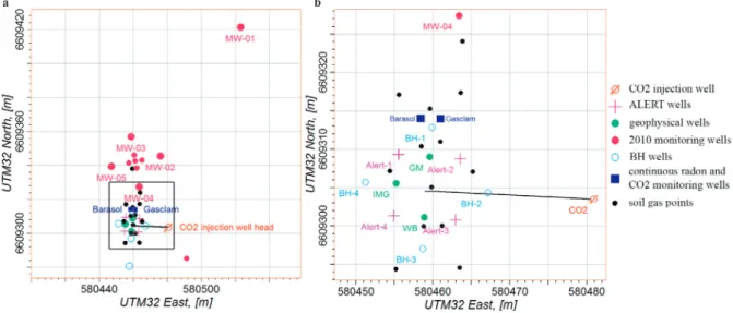
Figure 3. Layout of the experimental field site. (a) location of monitoring wells at the whole site scale; (b) close up

a b a b

(5)

3. Shallow injection experiment: Methods and results

3.1. Experimental setup

Given the available data on flow properties of the sediments from the site characterization, the expected behaviour of CO2 injected at about 20 m depth would be to form a rising bubble of gas less than 10 m in diameter.

It was decided to drill an oblique injection well to avoid disturbance of the sediment right above the injection point. The drilling process involves drilling a larger diameter hole in which injection tubes are inserted before extracting the larger diameter drilling tubes and injecting cement to fill the void around the injection tube. Achieving a good cementing performance with inclined wells and unconsolidated sediments is challenging and, as will be seen later, the construction of the injection well probably left a pathway for flow along the well at least part of the way to the surface. A map view of the injection well path and of the experiment layout is presented in Fig. 3.

From the 7th_{to 12}th_{September 2011, 1.7 tonnes of CO}

2 were injected with a well head pressure of 1.9-2 bar

(indicating gas entering the sediments at the expected depth). The injection of CO2 was continuous; however the

rate was increased in four incremental stages from 5 kg per hour up to 17.5 kg per hour (Fig. 4). The shallow subsurface was monitored using a combination of geochemical and geophysical techniques. This involved surface gas and bacterial activity monitoring, and downhole geochemical and geophysical monitoring. Table 1 provides a list of the tools used and corresponding mode of deployment.

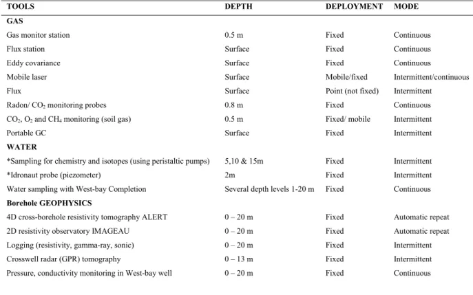
Table 1. List of tools used and corresponding mode of deployment.

TOOLS DEPTH DEPLOYMENT MODE

GAS

Gas monitor station 0.5 m Fixed Continuous

Flux station Surface Fixed Continuous

Eddy covariance Surface Fixed Continuous

Mobile laser Surface Mobile/fixed Intermittent/continuous

Flux Surface Point (not fixed) Intermittent

Radon/ CO2 monitoring probes 0.8 m Fixed Continuous

CO2, O2 and CH4 monitoring (soil gas) 0.5 m Fixed/ mobile Intermittent

Portable GC Surface Fixed Intermittent

WATER

*Sampling for chemistry and isotopes (using peristaltic pumps) 5,10 & 15m Fixed Intermittent

*Idronaut probe (piezometer) 2m Fixed Intermittent

Water sampling with West-bay Completion Several depth levels 1-20 m Fixed Continuous

Borehole GEOPHYSICS

4D cross-borehole resistivity tomography ALERT 0 – 20 m Fixed Automatic repeat 2D resistivity observatory IMAGEAU 0 – 20 m Fixed Automatic repeat Logging (resistivity, gamma-ray, sonic) 0 – 20 m Fixed Intermittent Crosswell radar (GPR) tomography 0 – 13 m Fixed Intermittent Pressure, conductivity monitoring in West-bay well 0 – 20 m Fixed Continuous

(6)

Figure 4. Injection rate during shallow injection test.

3.2. Near surface gas measurements

Soil gas samples were collected periodically from stainless steel probes or fixed metal tubes both within and outside the central injection area (Fig. 3). CO2 and other gases were measured in the field using portable Infra Red

(IR) analysers and selected samples measured in a field lab with a micro gas chromatograph. Radon (Rn) was also measured on selected points. CO2 concentrations were measured continuously at 4 locations and 2 continuous Rn

probes were deployed. CO2 flux measurements were made across the site using a portable flux meter (closed

accumulation chamber method) and measured at 4 locations continuously (2 of these were switched during the experiment to monitor venting of gas to atmosphere). Flux was also measured by eddy covariance. Atmospheric CO2 was measured at fixed locations, and on a limited number of mobile traverses, using an open path laser

analyser.

Changes in near surface gas concentrations and flux from systematic surveys, and observations in the fixed monitoring tubes and shallow water wells, identified areas of CO2 leakage (Fig. 5). However, measurements of gas

concentration and flux taken within the central area did not detect any leakage. Leakage was detected outside this area to the E (at 14.51 on the 8th_{September), NE (at 15.00 on the 10}th_{September) and NNE (at 10.00 on the 12}th

September) of the injection point (Fig. 5). The very large increases in CO2 concentrations and flux, and the ratios

of CO2 to O2 and N2, indicated a dilution of O2 and N2 by injected CO2 rather than near surface biological

production of CO2 (where O2 would decline in a 1:1 relationship with CO2 increase, whereas N2 would be

unaffected).

The maximum flux observed approached 2000 g m-2_d-1_{. This is similar to flux rates observed at natural CO} 2

vents (e.g. [6,7,8]). An estimate can be made of the total known gas escape to the atmosphere during the experiment based on the averaged daily survey measurements and the areas covered. This gives a total figure of 40-70 kg during the measurement period. This figure is likely to be an underestimate, as other small leakage areas may not have been detected, but it is worth noting that this would only equate to less that 5% of the total injected CO2.

Carbon isotopic ratios indicated some leakage of injected CO2 in the central area above the toe of the injection

well, but quantities must have been small because they were not detected by gas concentrations or fluxes.

3.3. Subsurface water monitoring

Borehole sampling: Water monitoring was performed through extraction of samples from (1) sampling ports

installed along the ALERT boreholes at depths of 5 m, 10 m and 15 m, (2) the 2010 groundwater monitoring wells and (3) four monitoring wells drilled for that purpose (BH, Fig. 3). Direct quantification of pH, T, redox potential, electrical conductivity and dissolved O2 was done in order to determine if further analysis was required. High

frequency sampling parameters were: alkalinity, dissolved ion contents (major and trace elements) and isotope ratios. At lower frequency, samples were obtained for subsequent detailed isotope analyses. Continuous records of pH, T, redox potential, electrical conductivity, dissolved O2 were also obtained in a 2 m borehole (BH01, Fig. 3)

(7)

Figure 5. (a) Soil gas concentrations data taken on 12 September showing 3 areas of gas escape E, NE and NNE of the main injection point; (b) corresponding soil gas flux data.

Westbay multilevel groundwater characterization and monitoring: The Westbay system is a modular

multilevel groundwater monitoring device enabling the user to test for hydraulic conductivity, monitor fluid pressure and collect fluid samples from multiple zones. A Westbay device was installed in a borehole at the southern edge of the central injection zone (WB, Fig. 3).

3.4. Geophysical monitoring

Automated time-lapse Electrical Resistivity Tomography (ALERT): Four down-hole arrays with 32

electrodes per borehole (vertical separation 0.75 m), were installed to a depth of 24 m. The ALERT boreholes were placed in the corners of a square with a side length of 8 m. With the depth of CO2 injection being at 20 m, it was

expected that this geometry would place the whole volume of interest (from injection to surface) within the sensitive zone for ALERT imaging and volumetric monitoring. 4D ERT datasets were collected by BGS before, during and after CO2 injection in order to assess the spatial and temporal changes in electrical properties associated

with the injection and migration of CO2.

Down-hole electrical observatory: A down-hole electrical observatory was provided by imaGeau and installed

in a borehole at the western edge of the central injection zone. The observatory was equipped with permanent electrodes with a vertical spacing of 0.7 m. Time-lapse resistivity measurements were made automatically, enabling real-time tracking of resistivity in the vicinity of the borehole over time.

Penetrating Radar (GPR): Time-lapse GPR recordings were made by CNRS Montpellier and BRGM between

two boreholes placed at the northern (GM) and the southern (WB) edges of the central injection zone. The method relies on dielectric permittivity contrasts and is thus very sensitive to changes in water saturation. GPR is known to be very effective in unconsolidated sedimentary environments, although signal penetration and hence depth of investigation may be limited by the presence of clay horizons.

Wireline logging: Repeated downhole logs of induction resistivity and gamma ray were recorded by CNRS

Montpellier in the GM and WB boreholes, providing physical property information at high vertical resolution

Soil Gas CO2 Concentratio n (%) Soil Gas CO2 Flux (g.m-2_.d-1₎ a b

(8)

Figure 6. Ground Penetrating Radar (GPR) 2D tomographies, showing evolution from baseline (leftmost plots) to post-injection – Day 8 (rightmost plots). The upper row shows the velocity distribution and the lower row the corresponding time-lapse relative variation in percent. South is to the left in each plot. The increase in GPR velocities observed on Day 4 denotes the presence of CO2 in gas phase. Follows a velocity

drop on Day 5, which is characteristic of the presence of dissolved CO2. The quick disappearance of the CO2 gas phase is assumed to be linked

to the breakthrough of the CO2 plume to the surface 30 m northward.

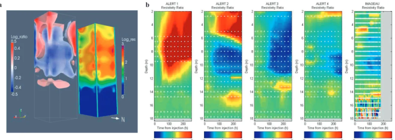
Figure 7. (a) 3D Resistivity model for day 11, viewed from the North East-facing ALERT borehole 2. The right hand image shows the resistivity distribution and the left hand image shows the change with respect to baseline. Regions in red have become more resistive and regions in blue have become more conductive; (b) Resistivity variation with time (ratio relative to baseline) for each individual ALERT borehole (1 to 4) and ImaGeau borehole (IMG). The rise of resistivity with time observed along ALERT 1 and at the surface on ALERT 2 is due to a probable contamination during baseline (released of brackish water from drilling) and is not associated with the CO2 migration. The

CO2 signature is the conductive plume associated to water-rocks interaction initiated by the lateral arrival of mainly dissolved CO2. 4. Data integration and discussion

In the CO2 injection process, a fraction of the CO2 will dissolve into the pore water. This is indicated in fluid

sampling data by an increase in electrical conductivity and a shift in water facies from SO4

to HCO3

-.

The fraction of CO2 that does not immediately dissolve will form a free gas phase within the pore spaces of the

sand and increase the bulk resistivity. This is suggested, in monitoring data, by the simultaneous increase in resistivity observed by ALERT and the downhole electrical observatory (ImaGeau), but complicated by mixing of different salinity waters, and indicated by the increase in radar velocity recorded in the cross-well GPR results around 72h after start of injection. This suggests that in the first 48 hours, the gas was being injected at a rate

(9)

greater than the dissolution rate and/or capacity of the system. During the first phase of the injection the viscous and capillary forces will dominate the gravity and the gas will spread radially from the injection point and create a bubble. However, the CO2 had found a path to the surface close to the line of the well within 27 hours, indicating

that there probably is a path of higher permeability along the well bore, bypassing the cement plugs. Migration of CO2 gas to the surface was otherwise determined and controlled by its interaction with the pore-water.

The injection rate was increased from 5 kg/hour on day one up to 17.5 kg/hour at the end of day two. On day three, the GPR results showed a sudden decrease in velocity which lasted until the end of the experiment (Fig. 6) and near surface gas measurements detected CO2 gas leakage to the north east of the site. This suggests that the free

gas-phase exceeded capillary pressure within the pore-spaces and the capacity of the near well bore pathway and found an additional escape route. As capillary forces were overcome, the CO2 plume advanced through the

sediments leaving a certain amount of dissolved and residual CO2. A very minor amount of CO2 did escape

vertically above the injection point as detected by sensitive isotopic methods but the main plume's migration path was much more convoluted, suggesting that it intersected internal layers of enhanced permeability, which allowed the gas plume to migrate laterally. This is supported by the ALERT results, which showed that in the middle and east of the site an area of high resistivity arose on day three and continued to develop during the rest of the experiment (Fig. 7). However, this would have been very difficult to interpret by itself without the more clear-cut changes in water chemistry and near surface gas data. Once a pathway was set up, the CO2 gas plume preferentially

took this path of least hydraulic resistance. Water chemistry suggests that dissolution effects were also very varied and that freshwater was displaced at the 10 m level to both 5m and 15 m depths [9]. Given the limited number of sampling points and measurement times, a general behaviour is derived but a detailed evolution of CO2 migration

cannot be established from this dataset.

The sand and gravel deposit at Svelvik contain channels with coarse to very coarse pebbles and cobbles (Fig. 2). Post-injection sampling indicates that a pebble/cobble bed occurs at 10 to 12 m depth in the shallow injection area. Baseline soil Rn concentrations formed E-W bands of varying concentrations. A central zone of higher Rn perhaps reflects a more permeable zone approximately parallel to the strike of the layering but this could also be related to higher concentration of Rn source material. The CO2 vents showed a strong NW-SE alignment, suggesting that the

permeable pathway continued up-dip at an oblique angle, consistent with a channel or lens acting as a preferential pathway for CO2 migration.

The amount of CO2 recorded at the surface is probably no more than about 5% of the total CO2 injected.

However, because of the nature of the experiment, only a proportion of the CO2 that reached the surface was

recorded directly. Nevertheless it is clear from these results that only a small proportion of the injected gas migrated to the surface and that a significant proportion dissolved into the groundwater. This is to be expected, since CO2 is highly soluble in water. Dissolution into the pore-waters is likely to be further enhanced by the

complex migration path encouraging mixing and dissolution [10].

The ALERT data showed an increase in resistivity from day 7 at the fresh water/saline water interface (Fig. 7). This might suggest downward displacement of the water column (locally) with an accompanying fall in the salinity of the water at that level. Such dilution was observed in water chemistry at 15 m depth [9].

Geochemical monitoring of water (mostly at depths of 5 m or greater) and isotope ratios in near surface soil gas were able to pick up compositional changes resulting from the injected CO2, near the injection point, that were not

apparent in the surface gas measurements and fluxes. This implies that the amounts of CO2 reaching the surface in

this central zone were very low and that geochemical techniques such as isotopic analysis were extremely sensitive indicators of CO2 leakage.

5. Lessons learned and recommendations

In this case, the CO2 breakout did not occur as predicted by modelling and the pre-injection knowledge of the

site. This is likely a consequence of the highly variable lamination and channelling of the sediments. There is a significant variation in grain size and structure within the sand and gravel deposit and this has affected CO2

migration. Ideally, for near surface CO2 escape experiments in such variable material, the geology needs to be

(10)

for CO2 migration would otherwise have been created. However, we should also consider if it is possible to

sufficiently characterise the subsurface (considering the technicality and cost) to make accurate model forecasts at this relatively small scale. The heterogeneity of the shallow subsurface is so great, the dynamics of the shallow aquifer are affected by so many external factors, such as infiltration and pumping, and the interactions between fresh and saline water so complex that point measurements cannot provide an accurate picture. Were the scale to be increased (i.e. injection depths closer to those of a real storage site) then small scale local variability might become of lesser importance in overall plume development.

It is likely that any discontinuity within the test site (natural or man-made) could act as a pathway for CO2 and

therefore care needs to be taken to set up monitoring equipment to take account of the possibility that CO2 breakout

may occur outside the main area of focus.

Mobile gas measuring equipment proved to be invaluable in picking up CO2 leakage at the surface. Apart from

the obvious advantages of mobility, it was also possible to produce results on site and the data could be interpreted without ambiguity.

The combination of geophysical techniques provided a rather consistent picture, with a good match to water properties. A particular success has been having a temporal and spatial capability. If financial constraints were no object, then an increase in the amount of geophysical data and the area covered, e.g. a bigger ALERT grid, and additional downhole and cross-hole monitoring (electrical resistivity logging, cross-well GPR, pressure logging), would have proved beneficial and might have allowed the CO2 migration to be tracked. However, none of these

techniques could be used below the freshwater/saline water interface due to the high resistivity contrast and this hampered the ability to track the CO2 plume from its source. Some electrical methods could be successful in saline

waters depending on the amount of gas and the salinity of the water. Therefore the presence of a saline aquifer will have implications for the design of the monitoring network.

Time constraints prevented adequate baseline characterisation. This was true for all techniques, but especially for the geophysical methods where, in most cases, only a short-term set of pre-injection measurements was made. This was not sufficient to define the background variability of the site (meteoric water flux, aquifer wind, tidal variations) and hence the subsequent interpretation of the data post-injection was made more difficult. Much more extensive baseline measurements should be a prerequisite of site characterisation.

Overall this experiment showed the difficulty in quantitatively assessing the amount of CO2 emitted from a

permeable body and (partially) migrating through the overlaying formation and ultimately to the atmosphere. This poses challenges for schemes such as the European Union trading system (EU ETS) which requires installations to detect, monitor and report their CO2 emissions. However, it should be noted that other methods may be applicable

at larger depths which are not tested here.

Acknowledgements

This publication is based on the results from the CO2FieldLab project, funded by CLIMIT research programme

(through Gassnova) and the French Direction Générale de la Compétitivité, de l'Industrie et des Services (DGCIS, France). The authors acknowledge the partners: SINTEF Petroleum Research, BGS, BRGM, Bureau Veritas, the Norwegian Geotechnical Institute (NGI), CNRS, imaGeau, Schlumberger Services Pétroliers and WesternGeco for their support.

References

[1] Directive 2009/31/EC of the European Parliament and of the Council of 23 April 2009. [2] Directive 2009/29/EC of the European Parliament and of the Council of 23 April 2009.

[3] Bakk A et al. 2012: CO2 Field Lab at Svelvik ridge: Site suitability Energy Procedia; 23: 306 – 312

[4] Sørensen R. Foreløpig beskrivelse til kvartærgeologisk kart SVELVIK – CL 083, M1:10 000. 1981: The Geological Survey of Norway, Report 1807/7.

[5] Melø T. Hydrogeology of the shallow aquifer at the Svelvik ridge. 2011: MSc thesis, University of Oslo, Norway.

[6] S.E. Beaubien, G. Ciotoli, P. Coombs, M.C. Dictor, M. Krüger, S. Lombardi, J.M. Pearce, J.M. West, The impact of a naturally occurring CO2 gas vent on the shallow ecosystem and soil chemistry of a Mediterranean pasture (Latera, Italy), International Journal of Greenhouse

(11)

[7] Martin Krüger, David Jones, Janin Frerichs, Birte I. Oppermann, Julia West, Patricia Coombs, Kay Green, Thomas Barlow, Robert Lister, Richard Shaw, Michael Strutt, Ingo Möller, Effects of elevated CO2 concentrations on the vegetation and microbial populations at a

terrestrial CO2 vent at Laacher See, Germany, International Journal of Greenhouse Gas Control, Volume 5, Issue 4, July 2011, Pages

1093-1098, ISSN 1750-5836, 10.1016/j.ijggc.2011.05.002.

[8] Lewicki JL, Oldenburg CM, Dobeck L, Spangler L (2007) CO2 leakage during two shallow subsurface CO2 releases. Geophys Res Lett

34:L24402. doi:10.1029/2007GL032047

[9] Gal F, Proust E, Humez P, Gilles B, Brach M, Koch F, Widory D, Girard J.-F. Inducing a CO2 leak into a shallow aquifer (CO2FieldLab

EUROGIA+ project): What can be learned from soil gas monitoring?, submitted for publication.

[10] Lindeberg E and Wessel-Berg D. 1997 Vertical convection in an aquifer column under a gas cap of CO2. Energy Conversation