Dynamics and control of electromagnetic satellite formations

(1)

Dynamics and Control of Electromagnetic

Satellite Formations

by

Umair Ahsun

B.Sc. in Electrical Engineering

University of Engineering & Technology, Lahore Pakistan (1996)

S.M. in Aeronautical and Astronautical Engineering

Massachusetts Institute of Technology, Feb. 2004 Submitted to the Department of Aeronautics and Astronautics

in partial fulfillment of the requirements for the degree of DOCTOR OF PHILOSOPHY

in

AERONAUTICAL AND ASTRONAUTICAL ENGINEERING

at the

MASSACHUSETTS INSTITUTE OF TECHNOLOGY

June 2007

Author

Graduate Research Assistant

Space Systems Laboratory

Certified By

David W. Miller Professor, Aeronautics & Astronautics Thesis Committee Chair/Thesis Advisor Certified By

Jonathan P. How

Associate Professor, Aeronautics & Astronautics

Thesis Committee Co-Chair Certified By _

James D. Paduano

,)Resarch Affiliate, Aeronautics & Astronautics Department

Thesis Committee Member Certified By _

Raymond J. Sedwick Principle Research Scientist, Aeronautics & Astronautics Thesis Committee Member Accepted By

Jaime Peraire ASSACHUSETTPST MS TECHNOLO E Chair, Committee on Graduate StudentsProfessor, Aeronautics & Astronautics

(2)

I

(3)

Dynamics and Control of Electromagnetic Satellite Formations

by

Umair Ahsun

Abstract

Satellite formation flying is an enabling technology for many space missions, especially for space-based telescopes. Usually there is a tight formation-keeping requirement that may need constant expenditure of fuel or at least fuel is required for formation reconfiguration. Electromagnetic Formation Flying (EMFF) is a novel concept that uses superconducting electromagnetic coils to provide forces and torques between different satellites in a formation which enables the control of all the relative degrees of freedom. With EMFF, the life-span of the mission becomes independent of the fuel available on board. Also the contamination of optics or sensitive formation instruments, due to thruster plumes, is avoided. This comes at the cost of coupled and nonlinear dynamics of the formation and makes the control problem a challenging one. In this thesis, the dynamics for a general N-satellite electromagnetic formation will be derived for both deep space missions and Low Earth Orbit (LEO) formations. Nonlinear control laws using adaptive techniques will be derived for general formations in LEO. Angular momentum management in LEO is a problem for EMFF due to interaction of the magnetic dipoles with the Earth's magnetic field. A solution of this problem for general Electromagnetic (EM) formations will be presented in the form of a dipole polarity switching control law. For EMFF, the formation reconfiguration problem is a nonlinear and constrained optimal time control problem as fuel cost for EMFF is zero. Two

(4)

different methods of trajectory generation, namely feedback motion planning using the Artificial Potential Function Method (APFM) and optimal trajectory generation using the Legendre Pseudospectral method, will be derived for general EM Formations. The results of these methods are compared for random EM Formations. This comparison shows that the artificial potential function method is a promising technique for solving the real-time motion planning problem of nonlinear and constrained systems, such as EMFF, with low computational cost. Specifically it is the purpose of this thesis to show that a fully-actuated N-satellite EM formation can be stabilized and controlled under fairly general assumptions, therefore showing the viability of this novel approach for satellite formation flying from a dynamics and controls perspective.

Thesis Supervisor: David W. Miller

(5)

Acknowledgements

I would like to acknowledge my advisor Dave Miller for his constant support and

guidance during my stay at Space Systems Lab. I would also like to thank my committee members Jonathan How, Jim Paduano and Raymond Sedwick for their helpful suggestions and critique that helped me to improve my research. I would like to thank my mother as no doubt her love and prayers helped me remain focused during my studies. And lastly and most importantly I thank my loving wife Sarah and our beloved son Arslan for their support and understanding.

(6)

(7)

List of Figures

Figure 1.1: Equal mass contours for Isp = 3000 thrusters and EMFF for a 10 years mission

life . ... 17

Figure 1.2: Thesis organization and interdependency of chapters... 23

Figure 2.1: Geometry of different reference frames ... 27

Figure 2.2: Geometry of the Rotated Frame Fr... 34

Figure 2.3: The main magnetic field generated by dynamo action in the hot, liquid outer core. Above Earth's surface, nearly dipolar field lines are oriented outwards in the southern and inwards in the northern hemisphere (source [25])... 43

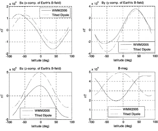
Figure 2.4: Comparison of the tilted dipole model and WMM2005 model for a polar circular LEO orbit at an altitude of 500 km (the longitude is fixed at -71*)... 48

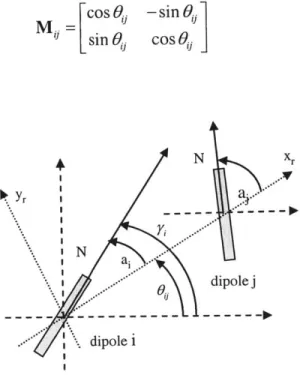
Figure 2.5: EMIFF coils, reaction wheel and coordinate frame definition for 2D dynamics ... 5 0 Figure 2.6: Geometry of steerable dipoles for magnetic force and torque computation.. 52

Figure 3.1: Two-satellite formation orbits... 76

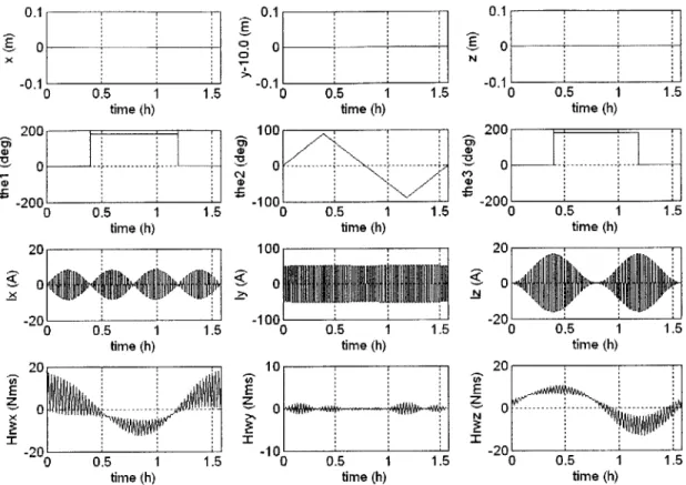
Figure 3.2: Follow er satellite results... 78

Figure 3.3: Follower satellite quaternions. ... 78

Figure 3.4: Different estimated parameters ... 79

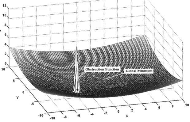
Figure 4.1: A potential function shape for vehicle 1. The obstruction function is at the location of the vehicle 0... 84

Figure 4.2: Reconfiguration results for a two-vehicle formation using APFM... 86

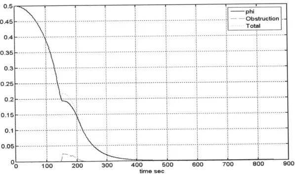
Figure 4.3: Values of the potential function along the trajectory of vehicle-I... 86

Figure 4.4: The decomposition of the motion planning problem. ... 87

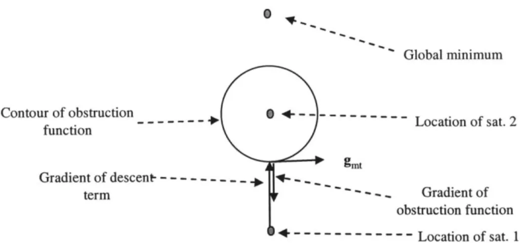
Figure 4.5: Case when the gradient of potential function can be zero... 88

Figure 4.6: Coordinate axes for testbed dynamics... 92

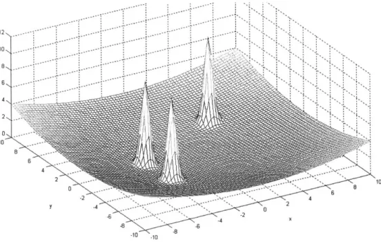
Figure 4.7: A potential function for one satellite in a 4-satellite formation. ... 96

Figure 4.8: Trajectories for the five-satellite formation reconfiguration... 103

Figure 4.9: Lyapunov functions for the five-satellite formation... 103

Figure 4.10: Trajectories for the four-satellite square formation reconfiguration... 104

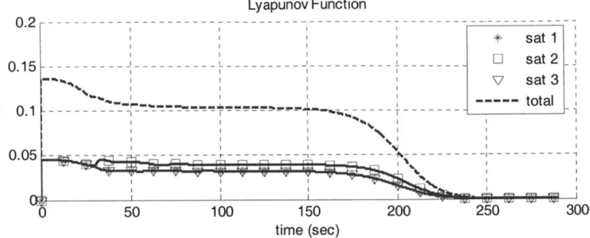
Figure 4.11: Lyapunov function for the four-satellite square formation. ... 105

Figure 4.12: Collision-free trajectories for a 2D, ten-satellite random formation... 106

Figure 4.13: Average simulation and computation-time values for different number of satellites in the random form ations... 107

Figure 4.14: A potential function for a 2-satellite formation in 2D with potential function shaping added... 109

Figure 4.15: Two-satellite formation reconfiguration result with PF shaping... 110

Figure 4.16: 2-satellite formation reconfiguration result without PF shaping... 111

Figure 5.1: Coil architecture for the Gen-X mission with block arrows showing the forces and torques acting on the dipoles... 120

(12)

Figure 5.2: Non-optimal slew results for the Gen-X mission... 123

Figure 5.3: Control profile for the optimal slew maneuver. ... 123

Figure 5.4: Control profile for the optimal slew maneuver. ... 124

Figure 5.5: Relationship between "direct" and "indirect" methods and the Covector M apping theorem [47]... 127

Figure 5.6: Direct shooting method for solving optimal control problems. ... 129

Figure 5.7: Results for two-satellite that switch places using the direct shooting method. ... 13 4 Figure 5.8: Cardinal functions (N=5) using Legendre Polynomials and LGL points (sq u ares)... 13 9 Figure 5.9: Infinity norm of the interpolation error for test functions given by Eq. (5.35) ... 14 2 Figure 5.10: Infinity norm of the derivative for test functions given by Eq. (5.35)... 143

Figure 5.11: Optimal trajectory results using the LPS method for a four-satellite form ation 90' C CW rotation...150

Figure 5.12: A ten-satellite random formation optimal trajectories results using LPS m eth o d ... 15 1 Figure 5.13: Trajectories generated using LPS method with N=55 for a two-satellite 900 slew m aneuver. ... 152

Figure 6.1: Trajectory following results for a two-satellite formation using exact Biot-Savart force-torque computation for the simulated system model, control and error sign als. ... 16 1 Figure 6.2: Trajectory following results for a two-satellite formation using exact Biot-Savart force-torque computation for the simulated system model. ... 162

Figure 6.3: Receding Horizon formulation using optimal cost-to-go function. ... 164

Figure 6.4: RH-formulation simulation results... 167

Figure 6.5: RH-formulation computation time during simulation... 167

Figure 6.6: Comparison of APFM and OTFM trajectories... 170

Figure A. 1: Nonlinear 3D Simulink simulation for electromagnetic formation... 181

Figure B. 1: Coordinate setup for control... 185

Figure B.2: Block diagram for the regulator setup. ... 186

Figure B.3: Standard State-Space setup for the regulator problem. ... 187

Figure B.4: Hf controller design setup... 192

Figure B.5: Weighting filters for error W1 and control effort W2... 193

Figure B.6: Closed-Loop TFs for H' synthesized controller. ... 194 Figure B.7: Time response of the closed-loop system to disturbances. Ix is total actuator

current, Ic is commanded current and IQ is the current resulting from quantization p ro cess... 19 5

(13)

Chapter 1 Introduction

1.1.

Motivation and Background

The term Satellite Formation Flying is used for systems that involve two or more spacecraft that fly near each other cooperatively to maintain their relative positions and orientations in order to execute a specific mission. The relative position and orientation of satellites can be fixed or time varying, e.g., a follower satellite may revolve around the leader satellite, while this leader-follower formation may itself be in an orbit around Earth. This distributed satellite architecture in turn enables a number of innovative space missions that are not possible or infeasible with a larger monolithic satellite structure [1], [2]. Some authors have defined the term satellite formation flying in a more precise way, e.g., Scharf et al [3] define satellite formation flying as "a set of more than one spacecraft whose dynamic states are coupled through a common control law. In particular, at least one member of the set must 1) track a desired state relative to another member, and 2) the tracking control law must at the minimum depend upon the state of this other member." This definition helps to differentiate the satellite formations from the satellite constellations (such as GPS) more easily.

Usually there is a very tight requirement for the control of relative position and orientation of the member satellites in the formation. This in turn may translate into

(14)

constant expenditure of fuel for near-Earth formations or at least fuel is required for formation reorientation. Therefore, the mission life span depends on the fuel available on board the satellites in the formation.

In order to elaborate on this point, consider an example of a two-satellite cross-track formation in a circular orbit around Earth. In such a formation the two satellites need to be kept at a constant distance from each other in a cross-track direction. It should be noted that such cross-track formations can be used in Synthetic Aperture Radar (SAR) applications in which the cross-track distance between the satellites acts as the baseline of the interferometer and can yield information about ground elevation differences [5].

For a circular orbit, the linearized relative dynamics of each satellite with respect to the formation center of mass orbit, which is in a natural Keplarian orbit, is given by Clohessy-Wiltshire equations (also called Hill's equations) [4]:

x- 2w09 =0

~9+-2+ 0 -3)o2y =0 (1.1)

where the coordinates (x, y, z) are local coordinates defined in a curvilinear reference frame that rotates as the formation orbits Earth. The y-direction points along the zenith direction, z-axis points along the orbital plane normal, and x-axis completes the right hand system (it points along the negative of the velocity vector for a circular orbit). The formation center of mass mean motion, or orbital frequency, is given by:

)0 = (1.2)

where ,ie is the gravitational constant of Earth (398,600.4418 x 109 m3_/s2₎_and_R

0 is the

(15)

For the cross-track formation, the two satellites are to be kept at a constant distance d from each other in the z-direction while the separation along the other two axes is zero. Using Eqs. (1.1), the total inertial force required to hold the formation can be shown to be:

IFI=

2 mm2 d n _(1.3)

m1 +m ₂

where m1 and m2 are the masses of the satellites. The forces are oriented in the

z-direction away from the orbital plane, effectively repelling the satellites from each other. It should be noted that these forces need to be applied constantly to hold the formation since each satellite in the formation is in a non-Keplerian orbit. Using the rocket equation

[23]:

M,= m, (eAv/sPi) (1.4)

the mass of propellant required to achieve a certain mission life can be estimated. In this equation mp and mf are the propellant mass and the final satellite mass (i.e. without propellant) respectively, AV is the "delta V" required to maintain the formation over the mission lifetime (it can be obtained by integrating Eq. (1.3)), I, is the specific impulse of the propulsion system and g is the acceleration due to gravity on the surface of Earth.

Similarly, using the dipole equation for two coaxial coils to generate the force given by [13]:

F =- -O(I (MRO)(M2R2)-- (1-5)

8)f p d

we can estimate the mass of the EMFF subsystem required to maintain the formation. In this equation F is the force generated between two coaxial coils separated by a distance d, MIR, and M 2R are the mass and radius product for coils one and two respectively,

(16)

I /p is the ratio of critical coil current and HTS (High Temperature Superconducting)

wire volume mass density and represents a technology factor. Using these two equations we can plot equal mass contours for EMIFF and thrusters, required to hold the formation in the cross-track direction, as shown in Figure 1.1 (for further detail see Reference [14]). Figure 1.1 shows the boundary when it is more mass-efficient to use 3000 second Isp thrusters versus EMFF. The horizontal axis is the cross-track offset (d/2), while the vertical axis is orbital period. The three curves correspond to different technology levels of the HTS wire. Three regions of interest exist. To the bottom right, the power needed to generate the requisite thrust is unavailable and EMFF is the only option. The region above the curves, and above the thruster limit line, corresponds to cross-track offsets and orbital periods where thrusters are more mass-efficient. Lastly, in the region above the thruster-limit line but below the curves, EMFF is more mass-efficient.

This comparison highlights several of the key benefits of EMIFF over thrusters as follows. First, EIFF does not have a mission lifetime limitation. Figure 1.1 shows that

EMFF is better as compared to thruste based systems for LEO and MEO (Medium Earth

Orbits) formations and for long duration missions. Another advantage of EMFF, highlighted by Eq. (1.5), is that adding an additional satellite to the formation improves performance of the EMFF subsystem whereas it does not benefit the thruster subsystem performance. Every time we add an extra, identical satellite and evenly distribute these satellites in the cross-track direction, the resulting reduction in neighbor-to-neighbor separation dramatically increases the magnetic force between neighbors. Note the change in the force given by Eq. (1.5) as a function of distance d. When a third satellite is added to the center of a two satellite formation, the neighbor-to-neighbor separation is divided

(17)

in half and the neighbor-to-neighbor force increases by a factor of sixteen (24). This increase in force allows the formation array to be grown in length, a capability unavailable with thrusters.

1 xlcpc (blue), 3xlcpc (green), 10fxlcpc (red)

Ic/pc=10x 45 ... ~ . .... ... .. . ... . .. . . .. 0 Ic/pc =x 1.5 07 CD

3

a_ 2 -Use-E Ff-100 200 300 400 500 600 700 800 900 Ff-1000 Cross-Track Offset [meters]

Figure 1.1: Equal mass contours for Isp = 3000 thrusters and EMIFF for a 10 years mission

life.

Although this example is a rather extreme one in which a steady expenditure of fuel is required, nevertheless it clearly highlights the impact of consumables on the mission lifetime. Since the satellites need to carry all of the fuel required over the mission lifetime (which means they would need to generate higher forces to hold the formation), using conventional thrusters can become infeasible for certain missions (thruster limit line in Figure 1.1).

(18)

It should be pointed out that another method of formation flying the satellites, without the used of consumables, is the concept of tethered formations in which different satellites in the formation are physically connected together with the help of tethers (see Reference [6] and references therein for a detailed description of this technique).

1.2. Overview of EMFF and Review of Previous Work on EMFF

The novel concept of Electromagnetic Formation Flight (EMFF) removes the mission life time dependency on the availability of fuel as highlighted in the last section. EMFF uses high temperature superconducting (HTS) wire technology to create magnetic dipoles on each satellite in the formation to generate forces and torques in order to maintain and reconfigure the satellite formation. A steerable magnetic dipole on each satellite can be created by using three orthgonogal coils on each satellite in the formation. Force on each satellite in the formation can be applied in any arbitrary direction by using these steerable magnetic dipoles. Since these forces are internal, the center of mass of the formation cannot be moved (momentum is conserved). This can be easily seen for a two satellite formation in which each satellite experiences equal but opposite force due to magnetic dipoles on each satellite. Since satellite formation control involves controlling the relative positions between the satellites, the inability to move the center of mass of the formation is not a limitation in itself. Another important aspect of EMFF is that whenever a shear force (i.e., a force that moves a satellite in the lateral direction with respect to the other satellite) acts on the satellite, a shear torque also acts on it. This shear torque needs to be countered by angular momentum storage devices such as reaction wheels or control moment gyros which can also perform the additional task of attitude control. Therefore, for an arbitrary N-satellite electromagnetic formation, all the relative degrees of freedom

(19)

can be controlled by using three orthogonal coils and three orthogonal reaction wheels. See references [7], [8] for a more detailed introduction to the concept of EMIFF.

Previous work on the dynamics and control problem associated with EMFF has shown that a two-satellite fully actuated electromagnetic formation that has three orthogonal coils and three orthogonal reaction wheels is fully controllable [9]. In this reference the dynamics (including the gyro-stiffening effect) for a two satellite formation in deep space (i.e. ignoring the gravitational terms, etc.) has also been derived. Models of the magnetic forces and torques between a general N-satellite electromagnetic formation are derived (both near-field and far-field) in Reference [10]. This reference also discusses ways of computing the dipole strengths to achieve the desired forces on the satellites in a formation. It also discusses the effects of Earth's gravitational and magnetic fields on

EMFF.

The control of a two satellite formation in LEO (Low Earth Orbit) based on phase-differences in the coil currents has been proposed by Kaneda et al [11]. In this method each coil is excited by a sinusoidal current with a constant frequency much higher than the orbital frequency and the desired force is provided by adjusting the phase difference between the two dipoles on the satellites in the formation. The sinusoidal variation in the coil current results in a net cancellation of the magnetic torque acting on each satellite due to the Earth's magnetic field. Although this method can be used for a formation of two satellites, it is not clear how it can be extended to formations of more than two satellites.

(20)

1.3. Research Objectives and Approach

As discussed in the previous sections, using EMFF allows the mission life to be independent of the available fuel on board. This comes at a cost in the form of complex nonlinear and coupled dynamics of the formation, making the control problem more challenging as compared to conventional thruster based formations.* There are two factors that increase the complexity of the dynamics and control problem associated with an electromagnetic formation. Firstly the forces and torques that act on the satellites due to the magnetic fields of other satellites in the formation are nonlinear, and secondly the dynamics of each satellite is coupled to that of every other satellite in the formation since changing the magnetic field strength on one satellite affects every other satellite in the formation with a non-zero magnetic dipole.

Previous work by Edmond Kong [12], Laila Elias [9] and Samuel Schweighart

[10] has shown that the EMFF concept is feasible for formation flying. This thesis

proposes to take this previous work a step further to find time-optimal trajectories, along with practical and feasible control schemes to track these trajectories. This will be done for a general N-vehicle electromagnetic formation in both deep-space and LEO.

In summary the objectives of this thesis are:

To develop dynamic models, suitable for the design and analysis of control laws for electromagnetic satellite formations for both near-Earth and deep space missions,

(21)

* To develop a framework in which control laws can be designed for electromagnetic formations for both LEO and deep-space missions,

e To develop algorithms for the generation of optimal trajectories for a general N-satellite electromagnetic formation,

e To develop algorithms for implementing the optimal trajectories in real-time, * And to test the models and control laws by using high-fidelity simulations.

The required research to achieve the above mentioned objectives can be broadly divided into four distinct areas:

1. Model development,

2. Control framework,

3. _{Optimal trajectory generation and real-time implementation,}

4. Verification in a simulated environment.

Although considerable work has been done in the area of model development, new models are still needed to meet the objectives. These new models will be developed using the Lagrangian technique for general electromagnetic formations. Using these models, the control of general formations will be developed by defining a framework or architecture in which different control formulations can be designed to meet the particular mission objectives. Since the "control cost" for EMFF is zero (it uses superconductors which consume no power and electrical power can be generated abundantly using solar energy), the optimal trajectories for EMFF are essentially minimum time trajectories constrained by the system dynamics and control saturations. From a system design point

(22)

of view, it is important to be able to generate these time-optimal trajectories and also to actually implement these in real time.

One way of real-time implementation of the optimal trajectories for complex nonlinear systems is to use the Optimal Trajectory Following Method (OTFM). Since the algorithms to generate optimal trajectories, for coupled nonlinear and constrained systems like EMFF, are computationally extensive. Therefore, from a real-time implementation point-of-view, optimal trajectories will be generated offline and then followed by separate trajectory following algorithms in real-time (see Chapters 5 and 6 for further detail). Another method of generating the trajectories, with a much lower computational burden as compared to OTFM, is to use feedback motion planning with the Artificial Potential Function Method (APFM) (see Chapter 4 for more detail). Both of these methods will be applied to general electromagnetic formations and the results will be compared.

1.4. Thesis Overview

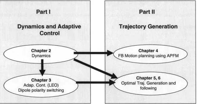
The rest of the thesis can be divided into two distinct parts as shown in Figure 1.2. Part I consists of Chapters 2 and 3 that describe the dynamics and control for general formations with a special emphasis on LEO. Chapter 2 derives the dynamics of general Electromagnetic (EM) formations using the Lagrangian method. These dynamics are suitable for simulating and designing control laws for general N-satellite EM formations in both LEO and deep-space. Chapter 2 also presents Earth's magnetic field models. Chapter 3 presents a framework in which different control laws can be developed for general EM formations. Using this framework, nonlinear adaptive control laws are derived in Chapter 3 for formation hold and trajectory following. These adaptive control

(23)

laws are suitable for both LEO and deep-space applications. This chapter also presents a practical method of managing angular momentum for general EM formations in LEO. This is done by switching the direction of the dipoles by 180 resulting in net cancellation of the torque due to the Earth's magnetic field. This method is termed dipole polarity

switching control law.

Part I Part i

Dynamics and Adaptive Trajectory Generation Control

Chapter 2 Chapter 4

Dynamics FB Motion planning using APFM

Chapter 3 Chapter 5, 6

Adap. Cont. (LEO) Optimal Traj. Generation and

Dipole polarity switching following

Figure 1.2: Thesis organization and interdependency of chapters.

Part II of the thesis consists of Chapters 4, 5 and 6 that discuss two different techniques of trajectory generation for nonlinear and constrained systems with specific application to general EM formations. Chapter 4 presents the Artificial Potential Function Method (APFM) for generating collision-free trajectories for general EM Formations. Chapters 5 and 6 present algorithms for implementing optimal trajectories for EMFF in real time. Chapter 5 presents the formulation of the optimal control problem for general EM formations. The solution to the optimal control problem is discussed using two "direct method" algorithms, namely Direct Shooting (DS) and the Legendre

(24)

PseudoSpectral method (LPS). Chapter 6 discusses two formulations, namely adaptive trajectory following and Receding Horizon (RH) (for implementing these optimal trajectories in real time). Thus Chapters 5 and 6 present a practical method, called the Optimal Trajectory Following Method (OTFM), of implementing optimal trajectories in real-time for coupled nonlinear and constrained systems. A comparison between APFM and OTFM is also presented in Chapter 6. The last chapter of the thesis presents a summary, and chapter-wise synopsis of key contributions of the thesis. Lastly some future directions for the research are discussed.

(25)

Chapter 2 Electromagnetic Formation Dynamics

The purpose of this chapter is to develop models that are necessary for simulating general electromagnetic formations in LEO as well as in deep space. These models will also be used to design control laws that will be tested in a fully nonlinear simulation environment. First the dynamic equations of a general electromagnetic formation in LEO will be derived, which will act as the nonlinear verification model. Next, attitude dynamics of the satellites in the formation will be presented. Then, deep-space 2D dynamics will be derived that are suitable for simulating formations for deep space missions. After that, the Earth's magnetic field model will be discussed; this is an essential element for simulating EM formations in LEO. The control laws need to be designed based on relative dynamics of the formation with respect to a leader satellite. These relative dynamics will be derived next and the tools required to simulate a general closed-loop formation in MatlabTM are discussed in Appendix A.

2.1. Translational Dynamic Model for LEO

In this section, nonlinear equations of translational motion for general electromagnetic satellite formations will be derived in the ECI (Earth Centered Inertial) frame. The use of the ECI frame results in simpler equations as opposed to using an orbital frame (that is colocated with the body of the satellite, also sometimes called Hill's frame). The

(26)

nonlinear dynamics derived here are useful for simulating a general satellite formation orbiting Earth. Moreover, for control purposes, these equations can be easily converted to relative equations of motion as presented later in this chapter.

2.1.1. Preliminaries

As discussed above, the equations of motion are developed in the ECI reference frame, which has its origin at the center of Earth, its x-axis points towards vernal equinox*, z-axis towards celestial north pole, and y-z-axis completes a right handed z-axis system. This axis system is not fixed to Earth (i.e., this frame does not rotate with Earth), although it moves as Earth orbits around the sun. For the purposes of this thesis, this frame can be assumed to be an inertial frame. Moreover, relative positional dynamics will be developed in an orbital frame FRO. This orbital frame is defined in such a way that its origin is attached to the center of mass of the formation with its y-axis aligned with the position vector RRO representing the position of the formation center of mass in the ECI frame. The z-axis points towards the orbital plane normal and the x-axis completes the right hand system (see Figure 2.1). Also a body frame, FBk , attached to the body of satellite-k with its origin at the center of mass of the satellite, is also defined which defines the orientation of each satellite in the inertial space.

In order to emphasize the peculiarities of electromagnetic formation control, we will restrict the dynamics to a circular orbit in order to avoid unnecessary details, although the same procedure can be used to extend the dynamics to elliptical orbits. The dynamics are derived for a general N-satellite electromagnetic formation such that the

* _{Vernal equinox is the direction of intersection of the Earth's equatorial plane and the plane of the Earth's} orbit around the sun (ecliptic) when the sun crosses the equator from south to north in its apparent annual

(27)

satellites are enumerated from 0 to N-1, with satellite-0 designated as the "leader" satellite. Satellitej Satellite i FBi Reference Orbit .. Formation c.m. "Leader" $ FBO

Figure 2.1: Geometry of different reference frames

For the derivation of the relative dynamics in the orbital frame it is necessary to represent the rate of change of a vector in two different reference frames. This can be

achieved by using the "Transport Theorem" [19]:

FI- FRO- FRO-FI

--r= r+- a> xr (2.1)

where F' denotes the ECI reference frame, FRO in frame F,

FRO - FI

ow denotes the angular velocity of frame

FI - io

r is the velocity as observed by an observer attached to frame F', and

FRO-r is the velocity observed by an observer attached to frame F7 _{and, x denotes cross}

(28)

2.1.2. Derivation of Translational Equations of Motion

Let Ri be the position vector of the ith satellite in a general N-satellite formation. Note

that Rk is a vector (a geometric object) that can have many representations in a given reference frame, for example a suitable representation for Ri in the ECI reference frame is:

Ri = xiax + yja, + za where:

(2.2)

a = Unit vector that points in the direction of the vernal equinox

a = Unit vector that is aligned with the celestial North Pole

a,= a, xa,

(Note that a general vector R1 is denoted in a given reference frame as R in the

following discussion).

The equations of motion will be developed using Lagrange's method [18], which is particularly useful for incorporating the gravitational perturbation terms and the magnetic force actuation terms. The velocity of the ith satellite, modeled as a point mass, is

N.

and its kinetic energy is given as:

T7 = mRTR, (2.3)

where mi is the mass of the satellite and R =[i,

j,

i]T . The potential energy of the

satellite in Earth's gravitational field is given as [15]:

V(R,,#)= YeMi Ri

[1

-k=2Jk Re R ) Pk(cos#)1 where: (2.4)

(29)

p,= Gravitational constant of Earth = 398,600.4418 x 109 m3/s2 R, = xi2+ y2 + z2

Re= Equatorial Radius of Earth = 6378136.49 m

JA = kth zonal harmonic of Earth (J2 = 0.00108263, J3 = -0.00000254, J4 =

-0.000000161)

Pk = Legendre polynomials of the first kind

#=

_{Angle between Earth's North Pole direction, i.e. a, and R,}

Note that Eq. (2.4) accounts for the non-spherical nature of the Earth (i.e. the equatorial radius is larger than the polar radius) and assumes that Earth is symmetrical

about its rotation axis hence other effects which are called tesseral and sectorial harmonics [16] are ignored. Although these effects may also be included in this expression, the J2 term is by far the dominant term and only this term will be included in

further analysis in this thesis for simplicity (although the Lagrange's method presented here allows for the addition of other terms in a straight forward manner). Equation (2.4), neglecting J3 and higher terms, gives the gravitational potential energy of the i satellite

as:

W (,) - i 1J2 (3 -1 (2.5)

where we have used the fact that cos(#) = zi / R, in the ECI reference frame.

In a similar fashion each satellite is immersed in the magnetic field generated by other satellites, which results in magnetic forces acting on the satellite. To incorporate the effect of these magnetic fields we need to determine the magnetic potential energy of a satellite due to the magnetic field of the other satellites in the formation. Modeling the

(30)

coils as magnetic dipoles, the magnetic potential energy of the ith satellite due to the magnetic field of the jth satellite is given as [17]:

V4'"(R , Rj)= -p1 Bi (r) (2.6)

where p is the dipole strength of the ith satellite (which is a vector quantity since we have assumed three orthogonal coils on each satellite hence giving us the ability to control current in each coil to orient this dipole vector anywhere in Euclidean space R3

r is a vector that gives the position of the

jth

satellite with respect to the ith satellite, B11 is the magnetic field strength due to satellite

j

at the location of the ith satellite, and "*" is

the dot-product operator. Note that the "dipole model" of the coils on the satellites is essentially a far-field approximation of the magnetic field and gives accurate results only when the distance between the satellites is many times the radius of the coils. See Reference [10] for a detailed derivation of the far-field model of the magnetic field. Since the principle of superposition applies to the magnetic field, to determine the total magnetic potential energy of the ith satellite due to the magnetic field of all the other satellites in the formation we simply sum up the individual contributions:

Vi'"(R, R,..., ) j(r)j (2.7)

Equation (2.7) will be developed further a bit later in this section due to the complexity of the resulting expressions.

Similarly the ith satellite also experiences the Earth's magnetic field and its magnetic potential energy due to Earth's magnetic field is given as:

VimE(R) = -,-i RBe(R) (2.8)

(31)

The equations of motion of the formation of N satellites can be derived using the Lagrange's equations [19]:

d(L4)-Lq

Q

(2.9)

where:

N-I N-I

L(q, 4)= System Lagrangian = I;(4i)- I{V7 (q,)+V/"(q)+VmE (qi)}

i=O i=O

q = Vector of generalized coordinates of the system = [qo qj q2 ... qN-1 ],

q= Generalized coordinates of the ith satellite = [xi yj ZiT]

Q

= Vector of generalized forces acting on the formation (such as solar pressure, drag, etc),

aL aL

Lq =-,and L, =.

aq aq

From the expression of the system Lagrangian given above, it can be argued that the equations of motion of the ih satellite can be developed by considering only the Lagrangian associated with it, i.e.:

d

-E _E

LQ - =

Q(2.10)

This is possible since the kinetic energy of the ith satellite depends only on its velocity and not on the generalized coordinates of any other satellite in the formation (as we are deriving the equations in an inertial reference frame). Carrying out the gradient and time derivative operations in Eq. (2.10) we get:

(32)

mi i (Vg"+V|"+V mE)=_, axi mi ya Vg +V'" +VmE In y Iv IymE) = QIY(2.11) m (g+m+VmE)=), azi

where the mass of the satellite, mi, is assumed to be constant and the Qj's represent the components of the external disturbance forces acting on the ith satellite in the ECI reference frame. Using Eq. (2.5), the gradient of the gravitational potential in the ECI frame can be expressed as:

Vi9 emxi p 22 xj(5z -_Ri2) _ _ - hemi [ + Re 2 2mi yx(5z2 - R)

1.

aqj R

+

2R7 yj (5 i (2.12)

Zi Zi (5Z2 - 3R )

Using Eq. (2.7), the gradient of the magnetic potential can be written as:

(V|"

(q,,q2'' N)]= - B(;) = Fi " (q,, pp)

(2.13)

N-1

I F,' (q,q,, p , pji) ₌FIFm(q ₁ N q 1'N)... j=O,j;i

where F),' is the magnetic force that acts on satellite-i due to satellite-j, j = qj - q, and

FIFm is the net magnetic force acting on satellite-i due to all other satellites in the

formation (the pre-superscript FI is added to emphasize that this force is in the ECI frame). Note that since the magnetic force is a conservative force, i.e. the change in the magnetic potential energy of a current carrying coil moving through the magnetic field is independent of the path taken by the coil, hence it can be written as the gradient of the magnetic potential. To see that this is the case, for a closed path the net work done is zero in the magnetic field:

(33)

f F.dr =0

and using Stoke's theorem in R3 _{[20], we can write the circulation integral of Eq. (2.14)}

as a curl (which is circulation per unit area at a point) as follows:

VxF=O (2.15)

Using the vector calculus identity:

V x (Vf)=0 (2.16)

for a scalar field f(x, y, z) in the Euclidean space R', the force F'" can be written as:

Fij q ,p V - (2.17)

Using the dipole approximation of the coils on each satellite, the magnetic field due to the

jth

satellite at the location of the ith satellite can be written as [9]:

Bi( 1 )= j ijy 3 (2.18)

Taking the gradient of Eq. (2.18), Eq. (2.17) can be written as:

Fi; (qqip11)= 4- r r r p,+-5 r, r (2.19)

Note that Eq. (2.19) gives the force on dipole i (present on satellite-i) due to dipole

j

(located on satellite-j). It depends on the distance between the two dipoles and the orientation of both dipoles in the inertial space. It is the dependence on the orientation of the dipoles that gives rise to the complexity of the expression for the force since the orientation of a dipole depends obviously on its orientation with respect to the body

(34)

frame of the satellite; it also depends on the orientation of the body axes in the inertial space. A simple algebraic form of the force equation can be obtained by defining a rotated frame, Fr, such that its x-axis is aligned with vector rq (see Figure 2.2).

PI -Z FR -y FBi -X ' FBi -z F4 -x Satellite -i _{Satellite -j}

Figure 2.2: Geometry of the Rotated Frame Fr.

In this rotated frame Fr, Eq. (2.19) can be expressed as:

2p - p-'/ p _{p p}

Fr F im A o - ,,'lJ-jX ()

p p -p p

where pre-superscript Fr is added to emphasize that this force is in frame Fr, and ry is the distance between the two dipoles and individual dipole strengths are expressed in their

Cartesian components, i.e. uk = [p , u p, ]T (k e {i, j}) in the rotated frame Fr. Note

(35)

respective orientations, hence the dependence of the force equations on the attitude of each satellite is implicitly embedded in the vector notation for j, and

Ad

.

Equation (2.20) highlights the two nonlinearities associated with using magnetic dipoles as actuators. The first of these nonlinearities is associated with the magnitude of the force, which scales inversely with the distance to the fourth power. The second of these nonlinearities is associated with both the magnitude and direction of the force as these depend upon the product of the individual components of the two dipoles. This second nonlinearity highlights the coupled nature of the magnetic actuation, i.e., modifying one dipole on one of the satellites in the formation results in the change of force on every other satellite in the formation with non-zero magnetic dipole.

Since we need the magnetic forces between the satellites in the ECI reference frame, we can use Eq. (2.19) directly or we can use Eq. (2.20) after multiplying it with the transformation matrix as follows:

FI m (qqjjAj)=FI TFr FrF7(qjqj,,,fl) (2.21)

where FI TFr is the orthogonal transformation matrix from the rotated frame to the inertial ECI reference frame. Such a matrix can be constructed since we need two principal

rotations of the ECI reference frame to align it with the rotated frame Fr. We first rotate the ECI reference frame about its z-axis by an angle Vf and then the resulting frame is rotated about its y-axis by an angle 6 to complete the orientation to frame Fr. Thus the transformation matrix from the ECI to the Fr frame can be written as [21]:

cos 6 0 -sin 6~ cos y sin y 01

FrTF= 0 1 0 _{sinyf cosyV} ₀

(2.22)

(36)

The inverse transformation from the Fr frame to the ECI reference frame F' is given simply by the inverse of the matrix FrTFI (which is equal to its transpose). The angles Vr

and 0 can be determined from the vector r as follows:

V/=tan- 1U-J

(2.23) 0= sin-1 rij-z

where rx, , _,, and r_, are the x, y and z-components, respectively, of the vector i in the ECI reference frame. Moreover, the magnetic dipoles of each satellite are needed in the ECI reference frame to use Eq. (2.19). For that we need the transformation matrices from the body frame of each satellite to the global ECI reference frame, which are described in the next section where the attitude dynamics will be discussed.

In a similar fashion, the gradient of the Earth's magnetic potential gives the force on the ith satellite due to the Earth's magnetic field. It will be shown later in this chapter (when Earth's magnetic field model will be discussed) that this gradient is extremely small as compared to other forces present in the system and can safely be ignored for the purposes of this thesis.

After combining these results with Eqs. (2.11), we obtain the translational dynamics of the i h satellite in the ECI reference frame as follows:

+ "mx. 3peReJ 2Mi (R 5z)x = Flix 01l"', N1"' . N ) + FI F

R, 2R,'

m +i m 3pR + i 1 N 1" FIF (2.24)

R i 2R,7

ii 3iue eJ2M (R2 2 Zi )zIFIm nq~iI+J

mi + pz3m 3pR+m (3R -5z )z = FI l'"'' qN I1 '"l N ) + FI Fdi

(37)

In these equations the notation has been changed from

Q

to Fd to emphasize that these are disturbance forces. Also note that Eqs. (2.24) include the J2 perturbations and

describe the translational dynamics of the ith satellite in the ECI reference frame. These equations, along with Eq. (2.19), can be used to simulate a general electromagnetic formation around Earth in the ECI frame and act as a nonlinear verification model for validation and testing of control laws developed in a later chapter. Moreover, these equations can be used to find the relative orbital dynamics of the satellites as discussed later in this chapter.

2.2. Attitude Dynamics Including Gyro-Stiffening Effects

As discussed previously a fully actuated satellite that has three orthogonal coils can control all the relative translational degrees of freedom. One side effect of applying any shear force using magnetic dipoles is that a torque also acts on the dipoles; therefore to control the attitude of a satellite and to counter this magnetic torque, each satellite in the formation needs to have angular momentum storage devices such as reaction wheels or Control Moment Gyros (CMGs). In this section, the attitude dynamics of a satellite in an electromagnetic formation will be presented in a simple form in order to highlight the control issues associated with attitude control. For example, it is assumed that the reaction wheels are mounted rigidly on the satellite (see [9] for modeling details for flexible mountings of the reaction wheels). It will be assumed that each satellite has three orthogonal reaction wheels and their gyro-stiffening effect will also be included in the dynamic equations.

For a rigid body rotating about its center of mass, the rate of change of the angular momentum is related to the applied torques and is given by the Euler equation [21]:

(38)

FI -- _(2.25)

where H is the total angular momentum of the satellite (including that of the reaction wheels), due to its rotation about its center of mass, and r is the external torque acting on the satellite. Using the Transport Theorem, Eq. (2.1), Eq. (2.25) can be written in terms of the rate of change of angular momentum in the body frame of the satellite as:

H+oxH =r (2.26)

where 0 is the angular velocity of the satellite in the inertial frame. The angular momentum of the satellite can be written as the sum of satellite body momentum (without reaction wheels spinning) and the reaction wheel momentum:

H = fiB +HRW (2.27)

Using Eq. (2.27) the attitude dynamics can be written as:

.-. m -d

HB +HRW+wx HB + OXHRW=T +8

where Vr is the magnetic torque acting on the satellite due to the magnetic field of other

-d

satellites in the formation and r is the disturbance torque (such as due to Earth's magnetic field). Moreover the rate of change of angular momentum of the reaction wheels acts as a torque on the satellite body frame, therefore we can write Eq. (2.28) as:

--- -m -d -(

HB+CXHB+WXHRW =T +T -TRW (2.29)

Let I and IRW be the inertia matrices of the satellite and reaction wheels,

respectively; then since fiB = Iw and HRW = IRWQ (where Q is the reaction wheel's

angular velocity vector), under the assumptions that the satellite body axes are aligned with the principal axes and the reaction wheels are also aligned with the satellite body axes, Eq. (2.29) reduces to following attitude dynamic equations:

(39)

I4+ (I3-I 2)'2J 3+ 2 IRW3Q3 W3IRW2Q2 T, + TdTRWx

I2)2+(I I3iw3+3IRW1R1 I RW3 ₃ my +dy RWy (230)

I3(>+(I2-I1)O420+4IRW2Q2 _{2 RW1} 1 m dz RWz

where o = [w4 (0₂ ₃]T is the angular velocity of the satellite in the ECI reference

frame, and

I, 0 0~

I= 0 12 0 = the inertia matrix for the satellite,

0 0 _{I3_}

IRW 1 0 0

IRW

r

IRW2 0 = the inertia matrix for the reaction wheels,

0 0 IRW3_

Tm [mx imy Imz ]T Td = [rdx Tdy Tdz ]T, and TRW = [TRWx TRWY TRWz ]T torques expressed in the satellite body frame (aligned with principal axes).

Note that Eqs. (2.30) are the simplest possible form of attitude dynamics for an

EMFF satellite with three orthogonal reaction wheels which are aligned with the principal

axes of the satellite. The orientation of the satellite in the inertial frame can be related to the body axis angular rates through either Euler angles or quaternions as follows [22]:

1 2 = -- Q(q)wo (2.31) 2 = M(0)-o (2.32) where:

q = [qO q, q2 q3] = a quaternion vector,

=[61 02 _{0 3}]T = Euler angle vector,

(40)

q1 q2 q3 Q(q)= -qo q3 -q2 -q3 -qo q1 q₂ q1 o-q_ 1 sinOtan02 cos6tan62 M(6)= 0 cos90 -sini .

O0 sin 0,sec602 cos01 sec02_

Note that by using quaternions we can avoid the singularities present in using Euler angles, but if there are no large angle slews then Euler angles can be used as well, while avoiding the singularities.

2.2.1. Magnetic Torque

The magnetic torque term in Eq. (2.28) can be written as:

N-1

L

=

2.

(2.33)

j=O,ji

where rij is the magnetic torque acting on the satellite-i dipole due to the satellite-j dipole. This torque can be written as:

Tl Ap x Bj(r j) (2.34)

where the terms are as defined in Eq. (2.17). Again, as we did in the case of magnetic force, using the dipole approximation of the coils on each satellite, the magnetic torque on the ith satellite due to the jth satellite can be written using Eq. (2.18) as follows:

T oj x X ; (. - (2.35)

Again the expression for torque is complicated by the fact that torque depends upon the orientation of both the source and target dipoles. As in the case of magnetic force, a

(41)

simple expression for magnetic torque can be derived in a rotated frame F' as defined for

Eq. (2.20):

Fr-m JU Jijj0+JiJi

Frin = o[4r 2p p, + p jz _(2.36) -pi-xti, - 2py,

Equation (2.36) highlights the nonlinearities associated with magnetic torque, which were also present with magnetic force, but with one important difference, namely the magnitude of the magnetic torque is inversely proportional to distance to the 3rd

power (as opposed to the force that depends on the distance to the 4th power). Therefore, the same magnetic field can produce much stronger torque, as compared to force, in a given dipole (the reason that magnetic torquers are used for satellite attitude control [23]) although for EMFF this may act as a negative factor during the system design process.

In order to compute the magnetic torque using Eq. (2.35), we need to express the magnetic dipoles 0, and Ct in the ECI reference frame as is the case for computing the force using Eq. (2.19). For that we need transformation matrices for each satellite to transform a vector from the body frame Fe' to the inertial frame F and vice versa. This can be achieved using the Euler angles as follows:

1 0 0 cosO2 0 -sin8 2 cos 0 sinO, 0~

FBiT F 3 sin 3 0 1 0 sin ₁ cos 6₁ 0 _(2.37)

_0 -sin03 cos0 3 sinO2 0 cos02 0 0 1

where FBiTFI is the transformation matrix from the ECI frame F' to the satellite-i body

frame FBi. Note that this is just one of the possible twelve ways in which the transformation matrix can be defined using Euler angles and this form is most common in aerospace applications (see reference [21] page 20). The transformation defined by Eq.