Dynamically reparameterized light fields

Dynamically Reparameterized Light Fields

by

Aaron Isaksen

Submitted to the Department of Electrical Engineering and Computer

Science

in partial fulfillment of the requirements for the degree of

Master of Science in Electrical Engineering and Computer Science

BARKER

at the

MASSACHUSETTS INSTITUTE OF TECHNOLOGY

November 2000

@

Aaron Isaksen, MM. All rights reserved.

MASSACHUSETTS _INSTITUTE

OF TECHNOLOGY

APRI2 42001

L-LIBRARIES

The author hereby grants to MIT permission to reproduce and

distribute publicly paper and electronic copies of this thesis document

in whole or in part.

A u th o r ...

Department of Electrical Engineering and Computer Science

November 28, 2000

Certified

bt

Leonard McMillan

Assistant Professor

---Thesis Supervisor

Accepted by ...

Arthur C. Smith

Chairman, Department Committee on Graduate Students

Dynamically Reparameterized Light Fields

by

Aaron Isaksen

Submitted to the Department of Electrical Engineering and Computer Science on November 28, 2000, in partial fulfillment of the

requirements for the degree of

Master of Science in Electrical Engineering and Computer Science

Abstract

This research further develops the light field and lumigraph image-based rendering methods and extends their utility. I present alternate parameterizations that permit

1) interactive rendering of moderately sampled light fields with significant, unknown

depth variation and 2) low-cost, passive autostereoscopic viewing. Using a dynamic reparameterization, these techniques can be used to interactively render photographic effects such as variable focus and depth-of-field within a light field. The dynamic parameterization works independently of scene geometry and does not require actual or approximate geometry of the scene for focusing. I explore the frequency domain and ray-space aspects of dynamic reparameterization, and present an interactive rendering technique that takes advantage of today's commodity rendering hardware.

Thesis Supervisor: Leonard McMillan Title: Assistant Professor

Acknowledgments

I would like to thank many people, agencies, and companies who helped with this

re-search. Firstly, I would like to thank my advisor Professor Leonard McMillan, whose

mentoring, leadership, and friendship was very important to me while I worked on

this project. Both Professor McMillan and Professor Steven Gortler of Harvard

Uni-versity were instrumental in developing key sections of this thesis and the dynamically

reparameterized light field work in general. Without their help, I would never have

been able to complete this work. Also, their help in writing the Siggraph 2000 paper

[13] and Siggraph 2000 presentation on this subject formed the textual basis for this

thesis.

This work was funded through support from NTT, Hughes Research, and a NSF

fellowship. In addition, Fresnel Technologies donated many lens arrays for the

au-tostereoscopic displays.

Thanks to Ramy Sadek and Annie Sun Choi for illustrations, assistance, support,

and proofreading of early versions of this thesis. Thanks to Robert W. Sumner for

his IOTEX experience and to Chris Buehler for many helpful light field discussions and

DirectX help. Thanks to Neil Alexander for the "Alexander Bay" tree scene and to

Christopher Carlson for permission to use Bump6 in our scenes.

I would like to thank Annie Sun Choi, Robert W. Sumner, Benjamin Gross, Jeffery

Narvid, the MIT LCS Computer Graphics Group, and my family for their emotional

support and friendship while I worked on this research. Their support made it possible

to keep going when things got especially difficult.

Once again, I would like to thank Professor Leonard McMillian, because he most

of all made this work possible.

Contents

1 Introduction 8

2 Background and Previous Work 12

3 Focal Surface Parameterization 18

4 Variable Aperture and Focus 22

4.1 Variable Aperture ... 22

4.2 Variable Focus ... .. . . .... ... . . 28

4.3 Multiple Focal Surfaces and Apertures . . . . 31

5 Ray-Space Analysis of Dynamic Reparameterization 39 5.1 Interpreting the Epipolar Image . . . . 39

5.2 Constructing the Epipolar Image . . . . 42

5.3 Real Epipolar Imagery . . . . 44

6 Fourier Domain Analysis of Dynamic Reparameterization 47 7 Rendering 52 7.1 Standard Ray Tracing . . . . 52

7.2 Memory Coherent Ray Tracing . . . . 53

7.3 Texture M apping . . . . 54

7.4 Using the Focal Surface as a User Interface . . . . 56

9 Results

62

9.1 Capture ... ... ... .... 62

9.2 C alibration . . . . 63

9.3 R endering . . . . 64

10 Future Work and Conclusion

66

A MATLAB code for Frequency-Domain Analysis

69

A.2 Viewing the EPI . . . . 71

A.3 Making the Filter ... ... 71

A.4 Filtering the Frequency Domain . . . . 72

A.5 Downsampling the EPI ... 73

A.6 Viewing the Frequency Domain Image . . . . 73

A.7 Viewing the Frequency Domain Image and Filter . . . . 74

A.8 Creating the Components of the Figure 6-1 . . . . 75

List of Figures

2-1 Parameterization of exit plane determines quality of reconstruction 3-1 Elements of my parameterization . . . . 3-2 Reconstructing a ray using the focal surface . . . .

4-1 4-2 4-3 4-4 4-5 4-6 4-7 4-8 4-9 4-10 4-11 4-12 4-13 4-14 4-15 5-1 5-2 5-3

Using the synthetic aperture system . . . . Examples of depth of field . . . . Changing the shape of the aperture filter . . . . "V ignetting" . . . .. "Seeing through objects" . . . .. Changing what appears in focus . . . . Freely-oriented focal planes . . . . Changing the focal surface . . . . An example using two focal surfaces . . . . Finding the best focal plane . . . . Creating a radiance function from a light field . . . . Using radiance images to find the best focal plane . . Reducing the number of focal surfaces . . . . Visualizations of the focal plane scores . . . . An example of four (reduced from eight) focal planes Ray-space diagrams of a simple light field . . . . Calculating the ray-space diagram . . . . Actual epipolar imagery . . . .

15 19 21 . . . . 23 . . . . 24 . . . . 26 . . . . 27 . . . . 27 . . . . 29 . . . . 30 . . . . 31 . . . . 32 . . . . 33 . . . . 34 . . . . 36 . . . . 37 . . . . 38 . . . . 38 41 43 45

5-4 Effects of shearing the focal surface . . . . 6-1 Frequency domain analysis of a simple scene . . . . 6-2 Frequency-domain analysis of a more complex scene

7-1 Rendering with planar homographies . . . .

8-1 A view-dependent pixel . . . . 8-2 The scene shown in Figure 8-3 . . . . 8-3 An autostereoscopic image . . . . 8-4 Reparameterizing for integral photography . . . . . 9-1 Real-time User Interface . . . .

10-1 Depth from focus . . . .

46 49 51 55 . . . . 60 . . . . 60 . . . . 61 . . . . 61 65 68

Chapter 1

Introduction

Traditionally, to render an image, one models a scene as geometry to some level of de-tail and then performs a simulation which calculates how light reacts with that scene. The quality, realism, and rendering time of the resulting image is directly related to the modeling and simulation process. More complex modeling and simulation leads to higher quality images; however, they also lead to longer rendering times. Even with today's most advanced computers running today's most powerful rendering al-gorithms, it is still fairly easy to distinguish between a synthetic photograph of a scene and an actual photograph of that same scene.

In recent years, a new approach to computer graphics has been developing: image-based rendering. Instead of simulating a scene using some approximate physical model, novel images are created through the process of signal reconstruction. Starting with a database of source images, a new image is constructed by querying the database for information about the scene. Typically, this produces higher quality, photorealistic imagery at much faster rates than simulation. Especially when the database of source images is composed of a series of photographs, the output images can appear with as high quality as the source images.

There are a variety of image-based rendering algorithms. Some algorithms require some geometry of the scene while others try to limit the amount of a priori knowledge of the scene. There is a wide range of flexibility in the reconstruction process as well: some algorithms allow translation, others only allow rotation. Often, image-based

rendering algorithms are closely related to computer vision algorithms, as computing structure from the collection of images is one way to aid the reconstruction of a new image, especially when translating through the scene. Another major factor in the flexibility, speed, and quality of reconstruction is the parameterization of the database that stores the reference images.

However, rendering is only part of the problem as there must be a image-based modeling step to supply input to the renderer. Some rendering systems require a coarse geometric model of the scene in addition to the images. Because of this re-quirement, people may be forced to use fragile vision algorithms or use synthetic models where their desire may be to use actual imagery. Some algorithms reduce the geometry requirement by greatly increasing the size of the ray database or by imposing restrictions on the movement of the virtual camera.

The light field [14] and lumigraph [7] rendering methods are two similar algorithms that synthesize novel images from a database of reference images. In these systems, rays of light are stored, indexed, and queried using a two-parallel plane parameter-ization [8]. Novel images exhibiting view-dependent shading effects are synthesized from this ray database by querying it for each ray needed to construct a desired view. The two-parallel plane parameterization was chosen because it allows very quick ac-cess and simplifies ray reconstruction when a sample is not available in the database. In addition, the two-parallel plane parameterization has a reasonably uniform sam-pling density that effectively covers the scene of interest. Furthermore, at very high sampling rates, the modeling step can be ignored.

Several shortcomings of the light field and lumigraph methods are addressed in this thesis. At low to moderate sampling rates, a light field is only suitable for storing scenes with an approximately constant depth. A lumigraph uses depth-correction to reconstruct scenes with greater depth variation. However, it requires an approximate geometry of the scene which may be hard to obtain. Both systems exhibit static focus because they only produce a single reconstruction for a given queried ray. Thus, the pose and focal length of the desired view uniquely determine the image that is synthesized.

This thesis shows that a dynamic reparameterization of the light field ray database can improve the quality and enhance the flexibility of image reconstruction from light field representations.

My goal is to represent light fields with wide variations in depth, without requiring

geometry. This requires a more flexible parameterization of the ray database, based on a general mathematical formulation for a planar data camera array. To render novel views, my parameterization uses a generalized depth-correction based on focal surfaces. Because of the additional degrees of freedom expressed in the focal surfaces, my system interactively renders images with dynamic photographic effects, such as depth-of-field and apparent focus. The presented dynamic reparameterization is as efficient as the static lumigraph and light field parameterizations, but permits more flexibility at almost no cost. To enable this additional flexibility, I do not perform aperture filtering as presented in [14], because aperture filtering imposes a narrow depth of field on typical scenes. I present a frequency domain analysis justifying this departure in Chapter 6.

Furthermore, my reparameterization techniques allow the creation of directly-viewable light fields which are passively autostereoscopic. By using a fly's-eye lens array attached to a flat display surface, the computation for synthesizing a novel view is solved directly by the optics of the display device. This three-dimensional display, based on integral photography [17, 23], requires no eye-tracking or special hardware attached to a viewer, and it can be viewed by multiple viewers simultaneously under variable lighting conditions.

In this thesis, I first describe pertinent background information, as well as the rele-vant previous work in this area of image-based rendering (Chapter 2). Next, I discuss the dynamic reparameterization approach to light field processing (Chapter 3) and explain of how the variable parameters of the system affect reconstruction of the light field (Chapter 4). It is instructive to look at dynamic light field reparameterization in other domains: I explore the effects of reparameterization in ray space (Chapter 5) and in the frequency domain (Chapter 6). I then discuss various methods to render dynamically reparameterized light fields (Chapter 7) as well as ways to display them

in three-dimensions to multiple viewers (Chapter 8). I describe the methods used to capture light fields as well as various particulars about my light fields (Chapter

9). Finally, I conclude with future work (Chapter 10) and various code samples for

Chapter 2

Background and Previous Work

This thesis examines the sampling and reconstruction methods used in light field rendering. Previous researchers have looked at methods to create light fields, as well as ways to deal with the high sampling rates required for light field representation. In this chapter, I discuss the major issues that arise when rendering from a ray database and what previous researchers have done to avoid these problems.

In recent years, researchers have been looking at ways to create images through the process of reconstruction. Chen and Williams were one of the first teams to look at image-synthesis-by-image-reconstruction; their system created new views by depth-based morphing between neighboring images [4]. However, this type of system does not allow the user to move far from where the images were taken. McMillan and Bishop advanced image-based rendering by posing the reconstruction process as querying a database of rays [15]. They suggested a 5-D plenoptic function to store and query rays of light that pass through a scene. Because the images were thought of as individual bundles of ray, they could move through a scene with more flexibility then previously available. However, because the system was 5-D, many more rays than necessary were represented in regions of open space.

Soon after, Gortler, Grzeszczuk, Szeliski, and Cohen published "The Lumigraph"

[7] and Levoy and Hanrahan published "Light Field Rendering" [14]. These papers

similarly reduced the 5-D plenoptic function to a special case of 4-D. In the 4-D case, the user can freely move around unobstructed space, as long as she doesn't pass in

front of any objects. This reduction of dimensions greatly increases the usability and storage of the ray database. In addition, the 4-D ray database can be captured simply

by moving a camera along a 2-D manifold.

Researchers have been looking at the ray database model of image-based rendering for some time, as it is a quite effective way to represent a scene. A continuous

representation of a ray database is sufficient for generating any desired ray. In such a system, every ray is reconstructed exactly from the ray database with a simple query. However, continuous databases are impractical or unattainable for all but the most trivial cases. In practice, one must work with finite representations in the form of discretely-sampled ray databases. In a finite representation, every ray is not present in the database, so the queried ray must be approximated or reconstructed from samples in the database.

As with any sampling of a continuous signal, the issues of choosing an appropriate initial sampling density and defining a method for reconstructing the continuous signal are crucial factors in effectively representing the original signal. In the context of light fields and lumigraphs, researchers have explored various parameterizations and methods to facilitate better sampling and rendering. Camahort, Lerios, and Fussell used a more uniform sampling, based on rays that pass through a uniformly subdivided sphere, for multi-resolution light field rendering [2]. For systems with limited texture memories, Sloan, Cohen, and Gortler developed a rendering method for high frame rates that capitalizes on caching and rendering from dynamic non-rectangular sampling on the entrance plane [21]. For synthetic scenes, Halle looked at rendering methods that capitalize on the redundant nature of light field data

[10]. Given a minimum depth and a maximum depth, Chai, Tong, Chan, and Shum

derived the minimum sampling rate for alias-free reconstruction with and without depth information [3]. Holographic stereograms are closely related to light fields; Halle explored minimum sampling rates for a 3-D light field (where the exit surface is two dimensional, but the entrance surface is only one dimensional) in the context of stereograms [11]. Shum and He presented a cylindrical parameterization to decrease the dimensionality of the light field, giving up vertical parallax and the ability to

translate into the scene [20].

The choice of a ray database parameterization also affects the reconstruction meth-ods that are used in synthesizing desired views. It is well understood for images that even with properly-sampled dataset, a poor reconstruction filter can introduce post-aliasing artifacts into the result.

The standard two-plane parameterization of a ray database has a substantial im-pact on the choice of reconstruction filters. In the original light field system, a ray is parameterized by a predetermined entrance plane and exit plane (also referred to as the st and uv planes using lumigraph terminology). Figure 2-1 shows a typical sparse sampling on the st plane and three possible exit planes, uv1, uv2, and uv3. To recon-struct a desired ray r which intersects the entrance plane at (s, t) and the exit plane at (u, v), a renderer combines samples with nearby (s, t) and (u, v) values. However, only a standard light field parameterized using exit plane uv2 gives a satisfactory

reconstruction. This is because the plane uv2 well approximates the geometry of the

scene, while uvl and uv3 do not.

The original light field system addresses this reconstruction problem by aperture filtering the ray database. This effectively blurs information in the scene that is not near the focal surface; it is quite similar to depth-of-field in a traditional camera with a wide aperture. In the vocabulary of signal processing, aperture filtering band-limits the ray database with a low-pass prefilter. This removes high-frequency data that is not reconstructed from a given sampling without aliasing. In Figure 2-1, aperture filtering on a ray database parameterized by either the exit plane uv1 or

uv3 would store only a blurred version of the scene. Thus, any synthesized view

of the scene appears defocused, "introducing blurriness due to depth of field." [14] No reconstruction filter is able to reconstruct the object adequately, because the original data has been band-limited. This method breaks down in scenes which are not sufficiently approximated by a single, fixed exit plane. In order to produce light fields that capture the full depth range of a deep scene without noticeable defocusing, the original light field system would require impractically large sampling rates.

r

I

E+E

₀₊

Figure 2-1: The parameterization of the exit plane, or uv plane, affects the

recon-struction of a desired ray r. Here, the light field would be best parameterized using

process of aperture prefiltering requires the high frequency data to be thrown away. To create a prefiltered ray database of a synthetic scene, a distributed ray-tracer [5] with a finite aperture renderer could be used to render only the spatially varying low frequency data for each ray. Also, a standard ray tracer could be used, and many rays could be averaged together to create a single ray. This averaging process would be the low-pass filter. In the ray-tracing case, one is actually rendering a high-resolution light field and then throwing away much of the data. Thus, this is effectively creating a lossy compression scheme for high-resolution light fields. If one wanted to aperture prefilter a light field captured with a camera system, a similar approach would likely be taken. Or, one could open the aperture so wide that the aperture size was equal to camera spacing. The system would have to take high resolution samples on the entrance plane: in other words, one would have to take a "very dense spacing of views. [Then, one] can approximate the required anti-aliasing by averaging together some number of adjacent views, thereby creating a synthetic aperture." [14] One is in effect using a form of lossy compression. The major drawback is that one has to acquire much more data than one is actually able to use. In fact, Levoy and Hanrahan did "not currently do" aperture prefiltering on their photographic light fields because of the difficulties in capturing the extra data and the limitation due to the small aperture sizes available for real cameras. Finally, if the camera had a very large physical aperture of diameter d, the light field entrance plane could be sampled every d units. However, lenses with large diameters can be very expensive, hard to obtain, and will likely have optical distortions.

To avoid aperture prefiltering, the lumigraph system is able to reconstruct deep scenes stored at practical sampling rates by using depth-correction. In this process, the exit plane intersection coordinates (u, v) of each desired ray r are mapped to new coordinates (u', v') to produce an improved ray reconstruction. This mapping requires an approximate depth per ray, which can be efficiently stored as a polygonal model of the scene. If the geometry correctly approximates the scene, the recon-structed images always appear in focus. The approximate geometry requirement imposes some constraints on the types of light fields that can be captured. Geometry

is readily available for synthetic light fields, but acquiring geometry is difficult for

photographically-acquired ray databases.

Acquiring geometry can be difficult process. In the Lumigraph paper, the authors

describe a method that captures a light field with a hand-held video camera [7]. First,

the authors carefully calibrated the video camera for intrinsic parameters. Then, the

object to capture was placed on a special stage with markers. The camera was moved

around while filming the scene, and the markers were used to estimate the pose. A

foreground/background segmentation removed the markers and stage from the scene;

the silhouettes from the foreground and the pose estimation from each frame were

used to create a volumetric model of the object. Finally, because the camera was

not necessarily moved on a plane, the data was rebinned into a two-parallel plane

parameterization before rendering. Using this method, the authors were only able to

capture a small number of small object-centered light fields.

Both the light field and lumigraph systems are fixed-focus systems. That is, they

always produce the same result for a given geometric ray

r.

This is unlike a physical

lens system which exhibits different behaviors depending on the focus setting and

aperture size. In addition to proper reconstruction of a novel view, I would like to

produce photographic effects such as variable focus and depth-of-field at interactive

rendering rates. Systems have been built to render these types of lens effects using

light fields, but this work was designed only for synthetic scenes where an entire light

field is rendered for each desired image [12].

In this chapter, I have discussed previous work in light field rendering and

ex-plained the problems that often arise in systems that render from a ray database.

Typ-ically, light fields require very high sampling rates, and techniques must be developed

when capturing, sampling, and reconstructing novel images from such a database. I

have discussed what previous researchers have developed for this problem.

Chapter 3

Focal Surface Parameterization

This chapter describes the mathematical framework of a dynamically-reparameterized-light-field-rendering-system

[13].

My dynamically reparameterized light field (DRLF) parameterization of ray databases

is analogous to a two-dimensional array of pinhole cameras treated as a single optical system with a synthetic aperture. Each constituent pinhole camera captures a fo-cused image, and the camera array acts as a discrete aperture in the image formation process. By using an arbitrary focal surface, one establishes correspondences between the rays from different pinhole cameras.

In the two-parallel-plane ray database parameterization there is an entrance plane, with parameters (s, t) and an exit plane with parameters (u, v), where each ray r is uniquely determined by the 4-tuple (s, t, U, v).

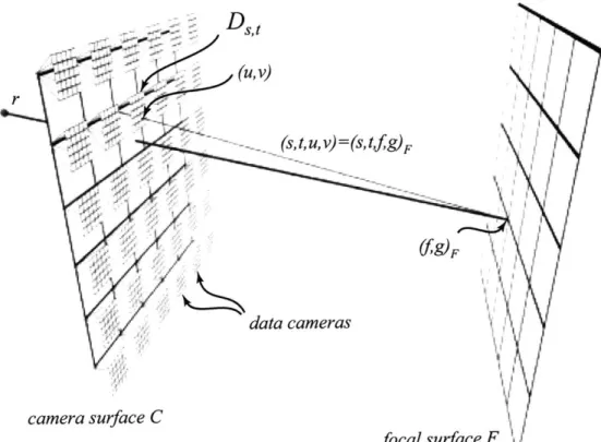
The DRLF parameterization is best described in terms of a camera surface, a

2-D array of data cameras and images, and a focal surface (see Figure 3-1). The

camera surface C, parameterized by coordinates (s, t), is identical in function to the entrance plane of the standard parameterization. Each data camera D,,t represents a captured image taken from a given grid point (s, t) on the camera surface. Each D,,t has a unique orientation and internal calibration, although I typically capture the light field using a common orientation and intrinsic parameters for the data cameras.

r

(S, , v)=(S,t g)F

data cameras

camera surface C

focal surface F

Figure 3-1: My parameterization uses a camera surface C, a collection of data cameras

D,,, and a dynamic focal surface F. Each ray (s, t, u, v) intersects the focal surface

g)F-Each pixel is indexed in the data camera images using image coordinates (u, v), and each pixel (u, v) of a data camera D,,t is indexed as a ray r = (s, t, u, v). Samples in the ray database exist for values of (s, t) where there is a data camera D8,,. The focal surface F is a dynamic two-dimensional manifold parameterized by coordinates

(f, g)F. Because the focal surface may change dynamically, I subscript the coordinates to describe which focal surface is being referred to. Each ray (s, t, u, v) also intersects the focal surface

F,

f,

-Each data camera

D,,

mapping tells which data camera ray intersects the focal surface F at

(f,

(f,

F,

PSt : (X, Y, Z) -+ (u, v) that describes how three-dimensional points are mapped

to pixels in the data camera

D,,,

Y, Z)

mapping MFjD is easily determined, M D P,tTF. Since the focal surface is defined at run time, TF is also known. Likewise, P,,t is known for synthetic light fields. For captured light fields, P,, is either be assumed or calibrated using readily available camera calibration techniques [24, 26]. Since the data cameras do not move or change their calibration, P,,t is constant for each data camera D,t. For a dynamic focal surface, one modifies the mapping TF, which changes the placement of the focal surface. A static TF with a focal surface that conforms to the scene geometry gives a depth-correction identical to the lumigraph [7].

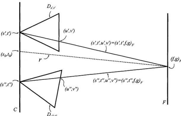
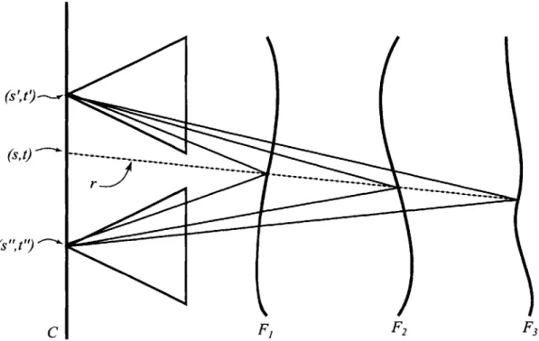
To reconstruct a ray r from the ray database, I use a generalized depth-correction. One first finds the intersections of r with C and F. This gives the 4-D ray coordinates (so, to,

f,

D,

,tl

D

",tl,

gives two rays (s', t', u", v") and (s", t", u", v") which are stored as the pixel (u', v') in the data camera D8,,, and (u", v") in the data camera D5

",t,.

(u',v')

F

C

Figure 3-2: Given a ray (s, t,

f,

(f,

Chapter 4

Variable Aperture and Focus

A dynamic parameterization can be used to efficiently create images that simulate

variable focus and variable depth-of-field. The user creates focused images of moder-ately sampled scenes with large depth variation and moderate sampling rates without requiring or extracting geometric information. In addition, this new parameterization gives the user significant control when creating novel images.

This chapter describes the effects that the variable aperture (Section 4.1) and variable focal surface (Section 4.2) have on the image synthesis. In addition, I explore some approaches that I took to create a system that has multiple planes of focus

(Section 4.3).

4.1

Variable Aperture

In a traditional camera, the aperture controls the amount of light that enters the optical system. It also influences the depth-of-field present in the images. With smaller apertures, more of the scene appears in focus; larger apertures produce images with a narrow range of focus. In my system synthetic apertures are simulated not to affect exposure, but to control the amount of depth-of-field present in an image.

A depth-of-field-effect can be created by combining rays from several cameras on

the camera surface. In Figure 4-1, the two rays r' and r" are to be reconstructed. In this example, the extent of the synthetic apertures A' and A" is four data cameras.

A'

desired camera

..

object

....

...

Figure 4-1: The synthetic aperture system places the aperture at the center of each desired ray. Thus the ray r' uses the aperture A' while r" uses A".

The synthetic apertures are centered at the intersections of r' and r" with the camera surface C. Then, the ray database samples are recalled by applying MF-D for all (s, t) such that D,,t lies within the aperture. These samples are combined to create a single reconstructed ray.

Note that r' intersects F near the surface of the virtual object, whereas r" does not. The synthetic aperture reconstruction causes r' to appear in focus, while r" does not. The size of the synthetic aperture affects the amount of depth of field.

It is important to note that this model is not necessarily equivalent to an aperture attached to the desired camera. For example, if the desired camera is rotated, the effective aperture remains parallel to the camera surface. Modeling the aperture on the camera surface instead of the desired camera makes the ray reconstruction more efficient and still produces an effect similar to depth-of-field (See Figure 4-2). A more realistic and complete lens model is given in [12], although this is significantly less efficient to render and impractical for captured light fields.

My system does not equally weight the queried samples that fall within the

Figure 4-2: By changing the aperture function, the user controls the amount of depth

of field.

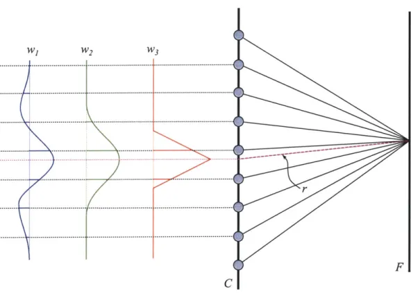
thetic aperture. Using a dynamic filter that controls the weighting, I improve the frequency response of the reconstruction. Figure 4-3 illustrates various attempts to reconstruct the pink dotted ray r = (so, to,

f,

w(x, y) to describe the point-spread function of the synthetic aperture. Typically w has a maximum at w(O, 0) and is bounded by a square of width 6. The filter is defined such that w(x, y) = 0 whenever x < -6/2, x > 6/2, y -6/2, or y J/2. The

filters should also be designed so that the sum of sample weights add up to 1. That i=L-6/2j

ii

The aperture weighting on the ray r = (SO, to,

f,

The center of each aperture filter is translated to the point (so, to). Then, for each camera D,, that is inside the aperture, I construct a ray (s, t,

f,

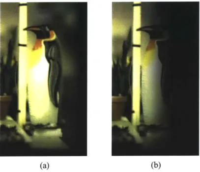
The dynamically reparameterized light field system can use arbitrarily large syn-thetic apertures. The size of the aperture is only limited to the extent to which there are cameras on the camera surface. With sufficiently large apertures, one can "see through objects," as in Figure 4-5. One problem with making large apertures occurs when the aperture function falls outside the populated region of the camera surface. When this occurs, the weighted samples do not add up to one. This creates a vignetting effect where the image darkens when using samples near the edges of the camera surface. For example, compare Figure 4-4a with no vignetting to Figure 4-4b. In Figure 4-4b, the desired camera was near the edge of the light field, so the penguin appears dimmed. This can be solved by either adding more data cameras to the camera surface or by reweighting the samples on a pixel by pixel basis so the weights always add up to one.

. ....... ... ... ..... ... ............- . .... W1 W2 W3 ... ... ... I ... ... ... ... ... ... . ... ...

...

_...

...

...

r

F

; 2

...

...

...

...

...

...

...

...

...

_*1

...

_****'**

...

*

...

_*"*'4

C

Figure 4-3: By changing the shape of the aperture filter, the user controls the amount

of depth-of-field. In this figure, filter w, reconstructs r by combining 6 rays,

combines 4 rays, andW3 combines 2.

(a)

(b)

Figure 4-4: A vignetting

a light field.

effect can occur when using large apertures near the edge of

Figure 4-5: By using a very large aperture, one can "see through objects.".

4.2

Variable Focus

Photographers using cameras do not only change the depth-of-field, but they vary what is in focus. Using dynamic parameterization, it is possible to create the same effect at run-time by modifying the focal surface. As before, a ray r is defined

by its intersections with the camera surface C and focal surface F and are

writ-ten (so, to,

f,

f,

-When the focal surface is changed to F', the same ray r now intersects a different focal surface at a different point

(f',

for the ray r. The new mapping MF'jD gives a pixel (u', v') for each camera D,, within the aperture.

In Figure 4-8, there are three focal surfaces, F1, F2, and F3. Note that any single

ray r is reconstructed using different sample pixels, depending on which focal surface is used. For example, if the focal surface F, is used, then the rays (s', t', u' , v' ) and

(s", t", u", v") are used in the reconstruction.

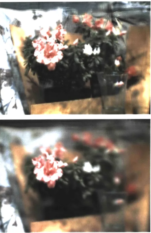
Note that this selection is a dynamic operation. In the light field and lumigraph systems, the querying the ray r would always resolve to the same reconstructed sam-ple. As shown in Figure 4-6, one can effectively control which part of the scene is in focus by simply moving the focal surface. If the camera surface is too sparsely sampled, then the out-of-focus objects appear aliased, as with the object in the lower image of Figure 4-6. This aliasing is analyzed in Section 6. The focal surface does not have to be perpendicular to the viewing direction, as one can see in Figure 4-7.

Many scenes can not be entirely focused with a single focal plane. As in Figure 4-8, the focal surfaces do not have to be planar. One could create a focal surface out of a parameterized surface patch that passes through key points in a scene, a polygonal model, or a depth map. Analogous to depth-corrected lumigraphs, this would insure that all visible surfaces are in focus. But, in reality, these depth maps would be hard and/or expensive to obtain with captured data sets. However, using a system similar to the dynamically reparameterized light field, a non-planar focal

Figure 4-6: By varying the focal surface, one controls what appears in focus.

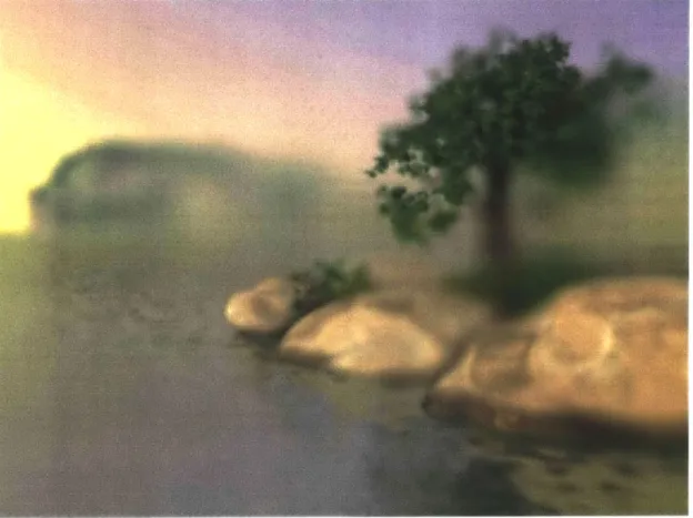
Figure 4-7: I have placed a focal plane that is not parallel to the image plane. In this

case, the plane passes through part of the tree, the front rock, and the leftmost rock

on the island. The plane of focus is seen intersecting with the water in a line.

r

C

F,

Figure 4-8: By changing the focal surfaces, I dynamically control which samples in

each data camera contribute to the reconstructed ray.

surface could be modified dynamically until a satisfactory image is produced.

4.3

Multiple Focal Surfaces and Apertures

In general, we would like to have more than just the points near a single surface

in clear focus. One solution is to use multiple focal surfaces. The approach is not

available to real cameras. In a real lens system, only one continuous plane is in focus

at one time. However, since the system is not confined by physical optics, it can have

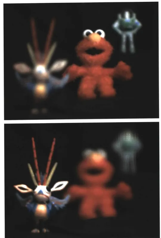
two or more distinct regions that are in focus. For example, in Figure 4-9, the red bull

in front and the monitors in back are in focus, yet the objects in between, such as the

yellow fish and the blue animal, are out of focus. Using a DRLF parameterization,

one chooses an aperture and focal surface on a per region or per pixel basis. Multiple

apertures would be useful to help reduce vignetting near the edges of the camera

surfaces. If the aperture passes near the edge of the camera surface, then one could

Figure 4-9: I use two focal surfaces to make the front and back objects in focus, while

those in the middle are blurry.

reduce its size so that it remains inside the boundary.

Using a real camera, this is done by first taking a set of pictures with different

planes of focus, and then taking the best parts of each image and compositing them

together as a post-process [18].

I now present a method that uses a

ray-tracer-based dynamically-reparameterized-light-field-renderer to produce a similar result by

expanding the ray-database-query-method.

Since a ray r intersects each focal surface F at a unique (f, g)F', some scoring

scheme is needed to pick which focal surface to use. One approach is to pick the

focal surface which makes the picture look most focused, which means the system

needs to pick the focal surface which is closest to the actual object being looked at.

By augmenting each focal surface with some scoring

which is the likelihood

F1 F2 F3 F4

03

Object

01

Figure 4-10: To find the best focal plane, I calculate a score at each intersection and

take the focal plane with the best score. If the scoring system is good, the best score

is the one nearest the surface one is looking at.

a visible object is near

one can calculate o- for each focal surface, and have

the system pick the focal point with the best score o-. In Figure 4-10, -2 would

have the best score since it is closest to the object. Note that an individual score

U(f, g)F

is independent of the view direction; however, the set of scores compared

for a particular ray r is dependent on the view direction. Therefore, although the

scoring data is developed without view dependence, view dependent information is

still extracted from it.

Given light-fields, but no information about the geometry of the scene, it is

pos-sible to estimate these scores from the image data alone. I have chosen to avoid

computer vision techniques that require deriving correspondences to discover the

ac-tual geometry of the scene, as these algorithms have difficulties dealing with

ambigu-ities that are not relevant to generating synthetic images. For example, flat regions

without texture can be troublesome to a correspondence-based vision system, and for

C

C

Figure 4-11: Creating a radiance function from a light field. If the radiance function

is near an object, then the function is smooth. If the radiance function is not near

an object, it varies greatly.

these regions it is hard to find an exact depth. However, when making images from

a light field, picking the wrong depth near the same flat region would not matter,

because the region would still look in focus. Therefore, a scoring system that takes

advantage of this extra freedom is desired. And, because only the original images are

available as input, a scoring system where scores are easily created from these input

images is required.

One approach is to choose the locations on the focal surfaces that approximate

radiance functions. Whereas one usually uses light-fields to construct images, it is

also possible to use them to generate radiance functions. The collection of rays in

the ray database that intersect at (f,

is the discretized radiance function of the

point

If the point lies on an object and is not occluded by other objects, the

radiance function is smooth, as in the left side of Figure 4-11. However, if the point

is not near an actual object, then the radiance function is not smooth, as in the right

side of Figure 4-11.

To measure smoothness, one looks for a lack of high frequencies in the radiance

function. High frequencies in a radiance function identify 1) a point on a extremely

specular surface, 2) an occlusions in the space between a point and a camera, or

3) a point in empty space. Thus, by identifying the regions where the there are no high frequencies in the radiance function, we know the point must be near a surface. Because of their high frequency content, we might miss areas that are actually on a surface but have an occluder in the way.

Figure 4-12 shows a few examples of what these radiance functions look like. Each radiance image in column 4-12a and 4-12c has a resolution equal to sampling rate of the camera surface. Thus, since these light fields each have 16x16 cameras on the camera surface, the radiance images have a resolution of 16x16. Traveling down the column shows different radiance images formed at different depths along a single ray. The ray to be traversed is represented by the black circle, so that pixel stays constant. The third image from the top is the best depth estimate for the radiance image because it varies smoothly. To the left of each radiance image is a color cubes showing the distribution of color in each radiance image immediately to its left. The third distribution image from the top has the lowest variance, and is therefore the best choice.

Because calculating the radiance function is a slow process, the scores are found at discrete points on each focal surface as a preprocessing step. This allows the use of expensive algorithms to setup the scores on the focal surfaces. Then, when rendering, the prerecorded scores for each focal surface intersection are accessed and compared. To find the best focal surface for a ray, an algorithm must first obtain intersections and scores for each focal surface. Since this is linear in the number of focal surfaces, I would like to keep the number of focal surfaces small. However, the radiance functions are highly local, and small changes in the focal surface position gives large changes in the score. Nevertheless, the accuracy needed in placing the focal surfaces is not very high. That is, often it is unnecessary to find the exact surface that makes the object in perfect focus; we just need to find a surface that is close to the object. Therefore, the scores are calculated by sampling the radiance functions for a large number of planes, and then 'squashing' the scores down into a smaller set of planes using some function A(oa, . . ., oj+m). For example, in Figure 4-13, the radiance scores for 16 planes are calculated. Then, using some combining function A, the scores from these 16 planes

(a)

(b)

(c)

(d)

Figure 4-12:

(a,c)

Radiance Images at different depths along a single ray. The circled

pixel stays constant in each image, because that ray is constant. The third image

from the top is the best depth for the radiance image. (b,d) Color cubes showing

the distribution of color in each radiance image immediately to its left. The third

distribution image from the top has the lowest variance, and is therefore the best

choice.

01 02 03 04 F5 06 07 08 09 010 011 012 C13 014 015 016

X(a₁,G2,a3,a4) X(o5,a6,o7,o8) X(o9,o10,a1 1,012) X(a13,o14,a15,a16)

Figure 4-13: I compute scores on many focal surfaces, and then combine them to a

smaller set of focal surfaces, so the run-time algorithm has less scores to compare.

are combined into new scores on four planes. These four planes and their scores are

used as focal surfaces at run time. I chose to use the maximizing function, that is,

...

might provide better results.

Figure 4-14 shows two visualizations of the scores on the front and back focal

planes used to create the image in Figure 4-9. The closer to white, the better the

score

o,

which means objects are likely to be located near that plane. Figure 4-15b

is another example that was created using 8 focal planes combined down to 4.

(a)

(b)

Figure 4-14: Visualizations of the o- scores used on the front (a) and back (b) focal

planes for the picture in Figure 4-9. The closer to white, the better the score o-, which

means objects are likely to be located near that plane.

(a)

(b)

Figure 4-15: (a) Using the standard light field parameterization, only one fixed plane

is in focus. Using the smallest aperture available, this would be the best picture

I could create. (b) By using 4 focal planes (originally 8 focal planes with scores

compressed down to 4), I clearly do better than the image in (a). Especially note the

hills in the background and the rock in the foreground.

Chapter 5

Ray-Space Analysis of Dynamic

Reparameterization

It is instructive to consider the effects of dynamic reparameterization on light fields

when viewed from ray space [14, 7] and, in particular, within epipolar plane images

(EPIs) [1]. The chapter discusses how dynamic reparameterization transforms the

ray space representations of a light field (Section 5.1). In addition, I explore the ray

space diagram of a single point feature (Section 5.2). Finally, I present and discuss

actual imagery of ray space diagrams created from photographic light fields (Section

5.3).

5.1

Interpreting the Epipolar Image

It is well-known that 3-1D structures of an observed scene are directly related to

features within particular light field slices. These light field slices, called epipolar

plane images (EPIs) [1], are defined by planes through a line of cameras. The

two-parallel plane (2PP) parameterization is particularly suitable for analysis under this

regime as shown by [8]. A dynamically reparameterized light field system can also be

analyzed in ray space, especially when the focal surface is planar and parallel to the

camera surface. In this analysis, I consider a 2-D subspace of rays corresponding to

fixed values of t and g on a dynamic focal plane F. When the focal surface is parallel

to the camera surface, the sf slice is identical to an EPI.

A dynamically reparameterized 2-D light field of four point features is shown in

Figure 5-la. The dotted point is a point at infinity. A light field parameterized with the focal plane F1 has a sfi ray-space slice similar to Figure 5-1b. Each point feature in geometric space corresponds to a linear feature in ray space, where the slope of the line indicates the relative depth of the point. Vertical features in the slice represent points on the focal plane; features with positive slopes represent points that are further away and negative slopes represent points that are closer. Points infinitely far away have a slope of 1 (for example, the dashed line). Although not shown in the figure, variation in color along the line in ray space represents the view-dependent radiance of the point. If the same set of rays is reparameterized using a new focal plane F2 that is parallel to the original F1 plane, the sf 2 slice shown in Figure 5-1c

results. These two slices are related by a shear transformation along the dashed line. If the focal plane is oriented such that it is not parallel with the camera surface, as with F3, then the sf slice is transformed non-linearly, as shown in Figure 5-1d.

However, each horizontal line of constant s in Figure 5-1d is a linearly transformed (i.e. scaled and shifted) version of the corresponding horizontal line of constant s in Figure 5-1b. In summary, dynamic reparameterization of light fields amounts to a simple transformation of ray space. When the focal surface remains perpendicular to the camera surface but its position is changing, this results in a shear transformation of ray space.

Changing the focal-plane position thus affects which ray-space features are axis-aligned. This allows the use of a separable, axis-aligned reconstruction filters in conjunction with the focal plane to select which features are properly reconstructed. Equivalently, one interprets focal plane changes as aligning the reconstruction filter to a particular feature slope, while keeping the ray space parameterization constant. Under the interpretation that a focal plane shears ray space and keeps recon-struction filters axis aligned, the aperture filtering methods described in Chapter 4 amount to varying the extent of the reconstruction filters along the s dimension. In Figure 5-le, the dashed horizontal lines depict the s extent of three different aperture

00

(a)

S4

(e)

fi

fi

(d)

-- 'in"'

(f)

...

...

.

(g)

Figure 5-1: (a) A light field of four points, with 3 different focal planes. (b,c,d)

sf

slices using the three focal planes, F

, F

and F

. (e) Three aperture filters drawn on

the ray space of (b) (f) Line images constructed using the aperture filters of (e). (g)

Line images constructed using the aperture filters of (e), but the ray space diagram

of (c)

... ... ... ...

filters (I assume they are infinitely thin in the

fi

dimension). Figure 5-if shows three

line images constructed from the EPI of Figure 5-1e. As expected, the line image

constructed from the widest aperture filter has the most depth-of-field. Varying the

extent of the aperture filter has the effect of "blurring" features located far from the

focal plane while features located near on the focal plane are relatively sharp. In

ad-dition, the filter reduces the amount of view-dependent radiance for features aligned

with the filter. When the ray space is sheared to produce the parameterization of

Figure 5-1c and the same three filters are used the images of Figure 5-1g are produced.

5.2

Constructing the Epipolar Image

Arbitrary ray-space images (similar to Figure 5-1) of a single point can be constructed

as follows. Beginning with the diagram of Figure 5-2. Let P be a point feature that

lies at a position (PX, P,) in the 2-D world coordinate system. The focal surface F is

defined by a point FO and a unit direction vector

Fd.

Likewise, the camera surface C

is defined by a point So and a unit direction vector

I would like to find a relation

between

s

and

f

so that I can plot the curve for P in the EPI domain.

The camera surface is described using the function

So + SSd = S,

The focal surface is described using the function

Fo + f Fd= Ff

Thus, given varying values of

s,

S. plots out the camera surface in world coordinates.

Likewise, given varying values of

f,

Ff plots out the focal surface in world coordinates.

For sake of construction, let

s

be the domain and

f

be the range. Thus, we wish

to express values of

f

in terms of

s.

Given a value of

s,

find some point S.. Then

construct a ray which passes from the point S, on the camera surface through the

point P that intersects the focal surface at some point Ff. This ray is shown as the

zA

Focal Surface

f

F0

SS

So

Camera Surface

x

Figure 5-2: Calculating the

(s,

f)

pair for a point P in space. The focal surface is

defined by a point Fo and a direction

Fd.

Likewise, the camera surface is defined by

a point So and a direction

dotted line in Figure 5-2. The equation for this ray is

S,+ a(P - Ss) = Ff

This gives the final relation between

s

and

f

as

SO + SSd + a(P - So - SSd) = Fo + fFd

Because So, Sd, FO, and Fd are direction or position vectors, the above equation is a system of two equations, with three unknown scalars, s,

f,

f

f.

aP,+Sox(1

-a)

Solving the above system of equations for

f

Fox(Py - Soy - SSdy) - Foy(Px - SOx - SSdx) + Px(Soy + sSdy) - Py(Sox + sS&)

Fdy (Px - SOx - sSdx) - F& (Py - SOy - sSdy)

(5.1) Solving for s in terms of

f

S

(Fox

(5.2)

Fox

If we take the common case where Fd and Sd are parallel and both point along the s-axis, then Fdy = Sdy = 0, Fdx = Sdx = 1 and we can reduce equation (5.1) to

the linear form:

Fox(Py - Soy) - Foy(Px - Sox - s) + PxSoy - Py(Sox + s) (53)

-(PY - SoY)

5.3

Real Epipolar Imagery

Looking at epipolar images made from real imagery is also instructive. By taking a horizontal line of rectified images from a ray database (varying s, keeping t constant) it is possible to construct such an EPI. Three of these images are shown in Figure 5-3a. The green, blue, and red lines represent values of constant v which are used to create the three EPIs of Figures 5-3b-d.

In Figure 5-4, I show the effect of shearing the epipolar images using the example EPI imagery from Figure 5-3d. In Figure 5-4a, I reproduce Figure 5-3d. In this EPI, the focal plane lies at infinity. Thus, features infinitely far away would appear as vertical lines in the EPI. Because the scene had a finite depth of a few meters, there are no vertical lines in the EPI. When the focal plane is moved to pass through features in the scene, the EPIs are effectively sheared so that other features appear vertical. Figures 5-4b and 5-4c show the shears that would make the red and yellow