Direct Doppler broadening in Monte Carlo
simulations using the multipole representation
The MIT Faculty has made this article openly available.
Please share
how this access benefits you. Your story matters.
Citation
Forget, Benoit, Sheng Xu, and Kord Smith. “Direct Doppler
Broadening in Monte Carlo Simulations Using the Multipole
Representation.” Annals of Nuclear Energy 64 (2014): 78–85.
As Published
http://dx.doi.org/10.1016/j.anucene.2013.09.043
Publisher
Elsevier
Version
Original manuscript
Citable link
http://hdl.handle.net/1721.1/107884
Terms of Use
Creative Commons Attribution-NonCommercial-NoDerivs License
Direct Doppler Broadening in Monte Carlo
Simulations using the Multipole Representation
Benoit Forget, Sheng Xu, Kord Smith
June 24, 2013
Abstract
A new approach for direct Doppler broadening of nuclear data in Monte Carlo simulations is proposed based on the multipole representa-tion. The multipole representation transforms resonance parameters into a set of poles and residues only some of which exhibit a resonant behav-ior. A method is introduced to approximate the contribution to the back-ground cross section in an effort to reduce the number of poles needing to be broadened. The multipole representation results in memory savings of 1–2 orders of magnitude over comparable techniques. This approach pro-vides a simple way of computing nuclear data at any temperature which is essential for multi-physics calculations, while having a minimal mem-ory footprint which is essential for scalable high performance computing. The concept is demonstrated on two major isotopes of uranium (U-235 and U-238) and implemented in the OpenMC code. Two LEU critical experiments were solved and showed great accuracy with a small loss of efficiency (10-30%) over a single-temperature pointwise library.
Keywords. Monte Carlo; Doppler Broadening, Multipole Representation
1
Introduction
Most continuous-energy Monte Carlo particle transport codes rely on point-wise representation of the nuclear data for each nuclide. This provides an efficient way to evaluate cross sections by linear interpolation with a pre-defined level of accuracy. This representation facilitates the numerical convolution needed to compute the Doppler broadening using the SIGMA1 algorithm [Cullen and Weisbin, 1976]. This approach requires approximately 1GB to represent the cross section data for 400 nuclides at a single temperature. Cross sections at a given energy are then found using a binary search on the energy grid of each nuclide at each particle interaction. Recent work to accelerate the binary search procedure introduced the concept of using a unionized grid over all the nuclides [Lepp¨anen, 2009] or a system of pointers [Romano and Forget, 2013], while faster, the unionized grid exacerbates memory requirements.
The promise of using Monte Carlo methods beyond benchmarking activ-ities has brought a need for explicit temperature dependence of the nuclear data. When coupled to temperature distributions in a nuclear reactor, cross sections at many temperatures are needed, making storage requirements for di-rect temperature-dependent tabulations prohibitive, and repeatedly performing SIGMA1 is computationally intractable.
Trumbull [2006] studied this issue and suggested that datasets at every 5– 10K would provide the level of accuracy needed for simple interpolation between temperature points. Considering that the range of interest of an operating reactor is between 300K–3000K, an enormous amount (200–300GB) of data would needed. It should also be noted that resonance upscattering effects require 0K nuclear data to be treated correctly [Ouisloumen and Sanchez, 1991].
An alternative method was proposed that reduces the required temperature intervals to 50K by using a pseudo-material definition [Conlin et al., 2005]. The upper and lower bound temperature sets are mixed proportionally to the square root of temperature differences. This reduces the size of data to approximately 40–50GB.
Yesilyurt et al. [2012] took a different approach using a regression model over the entire energy and temperature ranges to define a 10–15 term temperature expansion. This approach amounts to storing a reference temperature dataset plus the expansion terms at each energy point for each reaction type which requires 10–15GB of storage, with little loss in efficiency. This approach was selected for implementation in MCNP [Martin et al., 2013].
Recently, Viitanen and Leppanen [2012] proposed a clever approach that reduces considerably the memory footprint by explicitly accounting for target velocities using rejection sampling. A majorant cross section is defined for each nuclide over a unionized energy grid and Doppler rejection is performed by sampling a target velocity. A single temperature dataset and the majorant cross section are needed, thus storage requirements are on the order of 1–2GB. This approach while attractive for some implementations has a few setbacks since it relies on delta-tracking and rejection sampling which impact efficiency. Recent work discusses some of the tradeoffs that can be made between accuracy and efficiency [Viitanen and Leppanen, 2013].
This paper proposes a completely different appraoch that relies on a little known nuclear data representation called the ”multipole representation” devel-oped by Hwang [1987]. Hwang extended an approach proposed by [de Saussure and Perez, 1969] in their representation of the collision matrix. They showed that transmission probabilities for the reaction channels of interest could be rep-resented by rational functions related to Adler-Adler parameters. Hwang was able to circumvent the s-wave limitation by recasting the rational function in momentum space instead of energy space which led to the multipole represen-tation. Using this approach, the convolution integral over target velocities can be performed analytically, eliminating the need for linearizing the nuclear data resulting in a massive reduction of storage. This paper demonstrates for the first time how the multipole representation can be used in Monte Carlo simulations to capture the temperature dependence of the nuclear data.
Section 2 presents an overview of the multipole representation. Section 3 in-troduces ways by which the number of poles can be reduced to make the method more efficient for direct Doppler broadening. Section 4 reviews the Faddeeva function evaluation. Section 5 discusses the OpenMC implementation for two uranium isotopes and Section 6 presents results on two critical benchmarks. Section 7 discusses some of the implications of the multipole representation for full-core reactor calculations. This paper demonstrates that Hwang was ahead of his time in developing an elegant Doppler broadening theory that only now has found a truly practical use.
2
Multipole Representation
The foundation of the multipole representation of Hwang arises from the fact that the collision matrix must be single-valued and meromorphic in momentum space. Additionally, every meromorphic function (i.e. a function that is well behaved except at isolated points) can be expressed as the ratio of well-behaved functions (i.e. holomorphic functions), where the roots of the denominator are called poles (i.e. a singularity) and the contour integral along a path inclosing a pole is called a residue. With this in mind, the channel-channel Reich-Moore transmission probabilities can be expressed as a rational function. The neutron-neutron channel transmission probabilities are shown in Equation 1 and the generic neutron to channel c transmission in Equation 2. Additional details on the collision matrix and R-matrix theory can be found in [Hwang, 1987].
ρnn= Pn2M −1(√E) P2M(√E) = N X λ=1 2(l+1) X j=1 rnλ(j) p(j)λ −√E (1) |ρnc|2= |P2M −1 c ( √ E)|2 |P2M(√E)|2 = N X λ=1 2(l+1) X j=1 Reh 2r (j) cλ p(j)λ −√E i (2) where M = (l + 1)N (3)
ρnn and ρnc are transmission probabilities, p (j)
λ are the poles of the complex
function P2M, P is an holomorphic function, r(j)cλ is the residue of channel c associated to resonance λ and pole j, rnλ(j)is the residue of channel n, N is the number of resonances in the Reich Moore representation, and the summation from 1 to 2(l + 1) represents the number of poles for a given resonance type. Each pole is associated with a line-shape function that will vary with the relative velocity between the neutron and the target. It should be made clear that the poles are always fixed and it is their associated function that varies. For an s-wave resonance (l = 0), there are two associated poles. One producing a well-behaved (i.e. smooth) contribution over the energy range of interest (10−5 eV to 20 MeV), and another that exhibits the resonant nature. Finding the poles is complicated since they correspond to the roots of a high-order complex polynomial with roots that are often quite close to each other in momentum space. Hwang developed the WHOPPER code to find all the complex poles citing the importance of good initial guesses and the need for quadruple precision [Hwang, 1987]. Once all poles and residues have been computed, the 0K neutron cross sections are computed as
σx(E) = 1 E X l,J N X λ=1 2(l+1) X j=1 Reh −ir (j) xλ p(j)∗λ −√E i (4) σt(E) = σp(E) + 1 E X l,J N X λ=1 2(l+1) X j=1 Rehexp(−i2φl) −irtλ(j) p(j)∗λ −√E i (5)
where the potential cross section is given by σp(E) =
X
l,J
4πλ2gJsin2φl (6)
r(j)xλ and rtλ(j) are the residues for reaction x and total cross section around res-onance λ, gJ is the spin statistical factor, p
(j)∗
λ is the complex conjugate of the
pole, and φlis the phase shift. In this form, the cross sections can be computed
by summations over angular momentum of the channel (l), channel spin (J ), number of resonances (N ) and number of poles associated to a given resonance type 2(l + 1).
2.1
Doppler Broadening
The beauty of the multipole representation is the simplicity by which Hwang was able to perform Doppler-broadening using the Solbrig kernel [Solbrig, 1961]. The Solbrig kernel is derived from the Maxwell-Boltzmann distribution but in momentum space. The Doppler-broadened cross sections take the following form σx(E, ξ) = 1 E X l,J N X λ=1 2(l+1) X j=1 Rehrx √ πW (z0) −−ir√πxC( p(j)∗λ √ ξ , √ E 2√ξ) i 2√ξ (7) σt(E, ξ) = σp(E)+ 1 E X l,J N X λ=1 2(l+1) X j=1 Renexp(−i2φl) h rt √ πW (z0) −−ir√πtC( p(j)∗λ √ ξ , √ E 2√ξ) io 2√ξ (8) with ξ = kT 4A; z0= √ E − p(j)∗λ 2√ξ (9)
where W (z0) is the Faddeeva function. Hwang notes that the correction term
C is negligible except at very low energies, details of which can be found in [Hwang, 1992]. Doppler broadening a cross section at a given energy E is thus reduced to a summation over all poles; each with a separate Faddeeva function evaluation.
2.2
WHOPPER with ENDF/B-VII
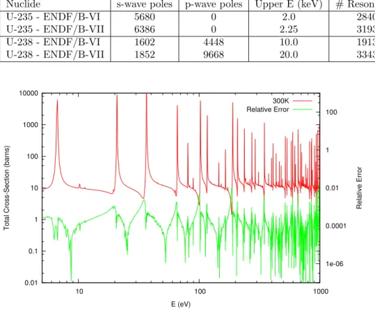
The WHOPPER code had, until now, only been tested on ENDF/B-V and ENDF/B-VI data [Hwang, 1992]. Minor changes were required in the code to accommodate the expanded number of resonances and associated poles, and a few obsolete Fortran functions needed to be replaced to suit selected compil-ers. Table 1 summarizes the ENDF/B-VI parameters from Hwang and the new ENDF/B-VII parameters for two uranium isotopes [Chadwick et al., 2011].
The U-238 resonance parameters were essentially doubled by extending the resolved range to 20 keV. The sheer number of p-wave resonances increased the computational cost substantially, but WHOPPER was still able to process all
Table 1: Pole parameter summary for U-235 and U-238
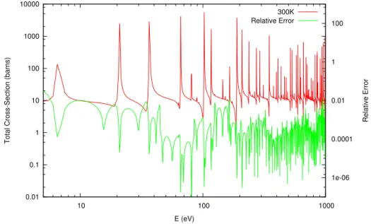
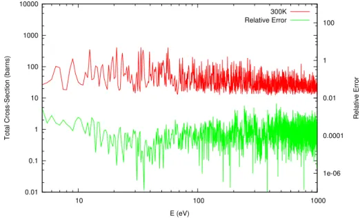
Nuclide s-wave poles p-wave poles Upper E (keV) # Resonances U-235 - ENDF/B-VI 5680 0 2.0 2840 U-235 - ENDF/B-VII 6386 0 2.25 3193 U-238 - ENDF/B-VI 1602 4448 10.0 1913 U-238 - ENDF/B-VII 1852 9668 20.0 3343 0.01 0.1 1 10 100 1000 10000 10 100 1000 1e-06 0.0001 0.01 1 100 Total C ross-Sec tion (bar ns) Relative Error E (eV) 300K Relative Error
Figure 1: U-238 comparison at 300K
of the poles. The U-238 calculation with ENDF/B-VII took approximately 6 hours on a 2.4 GHz Xeon processor using the Intel Fortran compiler. Most of the cost is associated with the quad-precision root-finding algorithm performed on a 64-bit architecture.
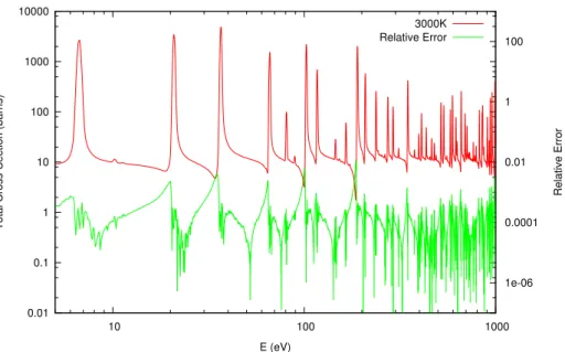
To illustrate the accuracy and completeness of the multipole method, com-parisons between NJOY [MacFarlane and Muir, 1999] and cross sections eval-uted with Equation 8 were performed at different temperatures using the ENDF/B-VII evaluation and are presented in Figures 1 and 2. The majority of the differ-ences are below the 0.1% interpolation error that was used in BROADR, with the exception of a few points where the differences are nearer to 1% when cross sections values are very low. Such differences are expected since the 0.1% in-terpolation criteria is not an absolute metric in NJOY when resonance integral tolerance is satisfied.
0.01 0.1 1 10 100 1000 10000 10 100 1000 1e-06 0.0001 0.01 1 100 Total C ross-Sec tion (bar ns) Relative Error E (eV) 3000K Relative Error
Figure 2: U-238 comparison at 3000K
Table 2: Poles of the 1029.325 eV p-wave resonance Pole 1 −3.2083095238830531e01 −1.6035743972167633e-04 i Pole 2 3.2083095238410557e01 +1.9807965569966046e-04 i Pole 3 3.2777164361828116e-10 +5.4415092287346283e02 i Pole 4 −1.689930997113225e-12 −5.4414252285191174e02 i
3
Understanding the pole representation
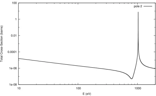
Looking at Table 1, it can seem somewhat far-fetched to replace a simple ta-ble lookup by a summation over thousands of poles each requiring their own Faddeeva function evaluation. Hwang had anticipated this reaction and offered some valuable suggestions by providing some insight on the behavior of the poles. The poles can be categorized in two general categories that he called fluctuating (i.e. showing a resonant nature in the energy range of interest) and non-fluctuating (i.e. smooth in the energy range of interest). Each resonance level in the Reich Moore formalism corresponds to one fluctuating pole, while the other poles associated to that resonance level are non-fluctuating. For example, let’s consider the 1029.325 eV p-wave (l = 1) resonance of U-238. Each p-wave resonance has four associated poles and those for this particular resonance are listed in Table 3.
Poles 1, 3 and 4 are considered non-fluctuating as seen in Figure 3, while pole 2 is considered fluctuating as illustrated in Figure 4. Non-fluctuating poles are characterized by negative real parts or by real parts very close to zero. The fluctuating pole is characterize by a positive real part that corresponds approximately to the square root of the resonance energy since poles are defined in momentum space.
-2e-05 0 2e-05 4e-05 6e-05 8e-05 0.0001 0.00012 0.00014 0.00016 10 100 1000 Total C ross-Sec tion (bar ns) E (eV) pole 1 pole 3 pole 4
Figure 3: Total cross-section contribution of non-fluctuating poles for U-238 p-wave resonance (1029.325 eV)
1e-08 1e-06 0.0001 0.01 1 100 10 100 1000 Total C ross-Sec tion (bar ns) E (eV) pole 2
Figure 4: Total cross section contribution of fluctuating pole for U-238 p-wave resonance (1029.325 eV)
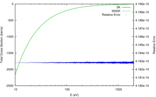
-2500 -2000 -1500 -1000 -500 0 10 100 1000 4.180e-10 4.181e-10 4.182e-10 4.183e-10 4.184e-10 4.185e-10 4.186e-10 4.187e-10 4.188e-10 4.189e-10 4.190e-10 Total C ross-Sec tion (bar ns) Relative Error E (eV) 0K 3000K Relative Error
Figure 5: Temperature independence of non-fluctuating poles of U-238
From the figures, we note that the non-fluctuating poles exhibit no resonant behavior in the positive energy domain, while the fluctuating pole represents the physical resonance. Also important is that simply neglecting poles is not an option since they can still make contributions to the base cross section over the entire energy range.
3.1
Pseudo-poles
Hwang proposed the use of a regression using rational functions to define a few pseudo-poles that can replace all non-fluctuating poles [Hwang, 1992]. This approach is consistent with the pole representation and allows for simple Doppler broadening of pseudo-poles, thus preserving the accuracy of the cross section. Preliminary analysis indicates that on the order of 10 pseudo-poles are needed for the ENDF/B-VII U-238 evaluation. This reduces the total number of poles to 3353 (926 s-waves, 2417 p-waves and 10 pseudo-poles). This strategy is certainly promising for improving computational efficiency, but not conclusive since the number of fluctuating poles is still proportional to the number of resonances.
3.2
Alternate Approach
Here, an alternate approach is proposed that combines both the ideas of an energy grid and approximations of non-fluctuating poles to further reduce the number of poles needed to evaluate cross sections at a specific energy point. The first thing to notice is that non-fluctuating poles have a very small tem-perature dependence that can be neglected in the 300–3000K range. Figure 5 illustrates error in the total cross section associated with neglecting the temper-ature dependence of the total contribution to σt from all non-fluctuating poles
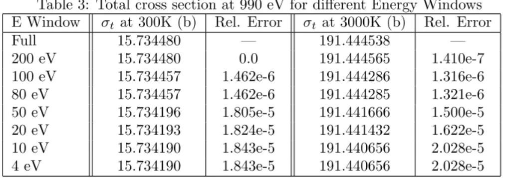
Table 3: Total cross section at 990 eV for different Energy Windows E Window σtat 300K (b) Rel. Error σt at 3000K (b) Rel. Error
Full 15.734480 — 191.444538 — 200 eV 15.734480 0.0 191.444565 1.410e-7 100 eV 15.734457 1.462e-6 191.444286 1.316e-6 80 eV 15.734457 1.462e-6 191.444285 1.321e-6 50 eV 15.734196 1.805e-5 191.441666 1.500e-5 20 eV 15.734193 1.824e-5 191.441432 1.622e-5 10 eV 15.734190 1.843e-5 191.440656 2.028e-5 4 eV 15.734190 1.843e-5 191.440656 2.028e-5
Another important point is that the temperature dependence of the cross section at a given energy only depends on a few neighboring resonances. This can be demonstrated by the following example in Table 3, where fewer and fewer fluctuating poles are broadened around 990 eV. This energy was selected due to its proximity to a large s-wave resonance at 991.7567eV. Table 3 presents cal-culated total cross section for two temperatures with decreasing energy window centered around 990 eV within which temperature dependence is considered.
A close look at these results indicates very little dependence on temperature from fluctuating poles far away from the given energy point. Additionally, Fig-ure 4 shows that fluctuating poles are very smooth away from the peak, thus making it possible to treat them as non-fluctuating poles away from the reso-nance. It should however be noted that the smaller energy windows presented in Table 3 do not always yield such accurate results. For certain energy points not in the immediate vicinity of a resonance, the errors can be much larger thus requiring a larger window. An in-depth analysis will need to be performed for each nuclide to determine an appropriate energy window and how much ac-curacy is needed in regions dominated by potential scattering and interference effects. The size of the energy window depends on the resonance level spacing and the width of the resonances. Equation 8 corroborates this observation by looking at the argument of the Faddeeva function. The√E −p(i)∗λ term becomes small far away from a pole, which enters rapidly the asymptotic region of the Faddeeva function, details of which are given in the next section.
The observations motivates the possibility of lumping fluctuating poles out-side a given energy window with the non-fluctuating poles, thus conout-siderably reducing the number of poles to be broadened. By grouping fluctuating poles over an energy window (Ω), neglecting the correction term and approximating all other poles as non-fluctuating within that same window, the cross section evaluation is thus reduced to:
σt(E) = σp(E) + p(E)poles6∈Ωl+
1 E X l,J X poles∈Ωl Rehexp(−i2φl)rt √ πW (z0) i 2√ξ (10) where p(E)poles6∈Ωl approximates the impact of all non-fluctuating poles and
fluctuating poles located outside the energy window Ωl. The subscript l is
added to account for the different range of each resonance type. For example, s-wave resonances have a much broader impact than p-waves and so forth.
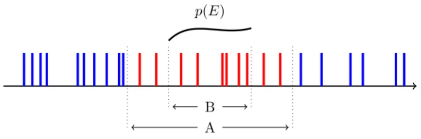
B A p(E)
Figure 6: Overlapping Energy Domains
3.2.1 Overlapping Energy Domains
The proposed approach for approximating the p(E) function is to use overlap-ping energy domains as illustrated in Figure 6. For a given energy interval A, all contributions from non-fluctuating poles and fluctuating poles (in blue) situated outside A are computed. Within a sub-interval B centered in A, the contribution from these poles is quite smooth and can be approximated using a low-order polynomial. The process is repeated until all sub-intervals B cover the entire resolved energy range. The use of overlapping domains eliminates edge effects of including or not including a resonance when evaluating near an interval boundary. When evaluating the cross section at energy E, one simply searches for the appropriate interval index, evaluate the low-order polynomial of that interval (p(E)), the potential scattering, and perform a summation over the fluctuating poles within the given interval (in red). Alternatively, the po-tential scattering component can also be lumped in p(E)poles6∈Ωl since it is very
smooth in the energy range.
4
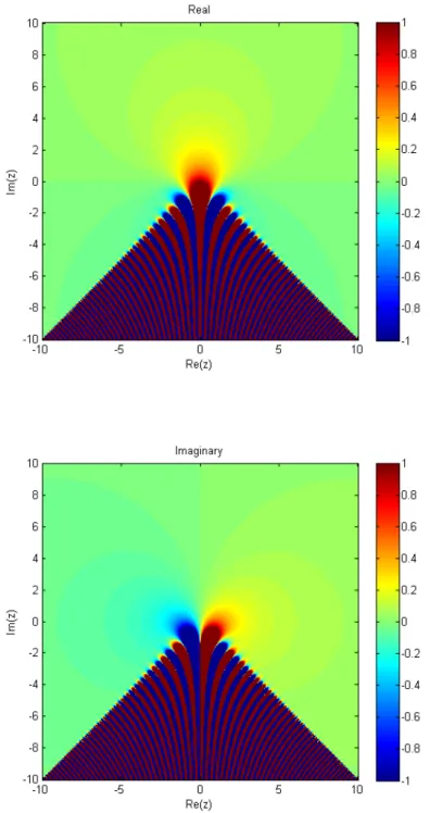
Faddeeva Function Approximation
The Faddeeva function, with complex argument z, is defined asW (z) = exp(−z2) erfc(−iz) (11) It has practical importance in many fields, thus efficient algorithms exist for its evaluation. The behavior of the Faddeeva function is presented in Figure 7 and appears quite unruly in certain regions of the complex plane. In the rigor-ous multipole representation of Hwang [1987], the argument z can require eval-uations anywhere in the complex plane. However, an interesting consequence of the approximations presented in this paper is that evaluations are only re-quired for the upper half of the complex plane where the behavior is much smoother.The fluctuating poles are defined such that the imaginary component is always greater than zero, which is not always the case for non-fluctuating poles. Additionally, Hwang suggested an approach in evaluating the asymptotic form of the Faddeeva function using a Gauss-Hermite quadrature for different ranges without much loss of accuracy for this given application [Hwang, 1992]. Thus computationally, not all Faddeeva function evaluations are equal within a given energy range. Poles further away from the given energy will require less quadrature points than those that are closer to that energy, and only poles in
close proximity will require an exact evaluation. This presents another possible optimization between the width of the energy window, the number of fluctuating poles to be broadened, and the desired level of accuracy needed.
5
Implementation in OpenMC
A simple implementation of the two major uranium isotopes was performed in OpenMC. The poles for both nuclides were processed using WHOPPER and a post-processing code was written to define overlapping energy domains from 5 eV to the respective upper bound of the resolved resonance range of each nuclide. At this time, focus was given to the resolved resonance range only. Capturing the thermal range is a bit more difficult and requires higher order expansions. An alternative approach using a few pseudo-poles for the thermal range is being considered. Thus, in this implementation, the remainder of the energy range is read from the standard ACE library. For U-238 an inner/outer energy window of 40/80 eV was selected for both s-wave and p-wave resonances since it provided a good compromise between accuracy and the number of poles to be broadened. On average, each energy window has four s-wave resonances and eight p-wave resonances. For U-235, an inner/outer energy window of 10/20 eV was selected, each with approximately 25 s-wave resonances. Ideally, all nuclides would have the same energy window, thus simplifying data access patterns. More research will be needed on that front as more nuclides are considered. The current implementation of using a uniform grid for a given nuclide is still quite efficient since the appropriate interval can be determined by a simple division rather than a binary search.
The temperature independent function p(E) was evaluated using a polyno-mial fit of low order. In most cases, a second order polynopolyno-mial proved sufficient, except at low energy where a third order polynomial was employed (below 85 eV for U-238 and 55eV for U-235). Figures 8 to 11 indicate the level of ac-curacy seen in the two uranium isotopes for two different temperatures. The comparison is made between the full multipole representation and the approx-imate representation on a 0.5 eV mesh. It should be noted that plotting cross sections on such a coarse uniform mesh will not capture the exact peaks of the resonance thus creating plots that are counter intuitive at first. The upper range was truncated at 1 keV for clarity.
The first thing to notice from Figures 8 to 11 is that the errors are very low at the location of resonances and can become a bit larger away from resonances. For both U-235 and U-238, the largest relative errors are about 1% and are located in regions with low cross section value (10 barns). Lower error values could be obtained by improving the polynomial fit for the non- fluctuating poles. The key benefit of the pole representation is in data reduction. In binary format, U-238 fluctuating poles and associated fitting coefficients for p(E) re-quire just under 325 kB, while the U-235 storage rere-quirements are just under 265 kB. This presents a huge reduction when compared to the linearized form of the ace files where the resolved resonance range takes up 10’s of MB for a single temperature.
0.01 0.1 1 10 100 1000 10000 10 100 1000 1e-06 0.0001 0.01 1 100 Total C ross-Sec tion (bar ns) Relative Error E (eV) 300K Relative Error
Figure 8: Comparison between rigorous multipole and approximate representa-tions for U-238 at 300K
0.01 0.1 1 10 100 1000 10000 10 100 1000 1e-06 0.0001 0.01 1 100 Total C ross-Sec tion (bar ns) Relative Error E (eV) 3000K Relative Error
Figure 9: Comparison between rigorous multipole and approximate representa-tions for U-238 at 3000K
0.01 0.1 1 10 100 1000 10000 10 100 1000 1e-06 0.0001 0.01 1 100 Total C ross-Sec tion (bar ns) Relative Error E (eV) 300K Relative Error
Figure 10: Comparison between rigorous multipole and approximate represen-tations for U-235 at 300K
0.01 0.1 1 10 100 1000 10000 10 100 1000 1e-06 0.0001 0.01 1 100 Total C ross-Sec tion (bar ns) Relative Error E (eV) 3000K Relative Error
Figure 11: Comparison between rigorous multipole and approximate represen-tations for U-235 at 3000K
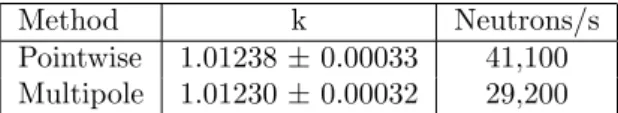
Table 4: LEU-SOL-THERM-001 benchmark - Eigenvalue and Computational Efficiency Method k Neutrons/s Pointwise 1.01238 ± 0.00033 41,100 Multipole 1.01230 ± 0.00032 29,200
6
Results
The approximated multipole implementation was tested on two low-enriched uranium (LEU) benchmarks from the International Criticality Safety Bench-mark Evaluation Project [NEA, 2009], namely 1) LEU-SOL-THERM-001 and 2) LEU-COMP-THERM-008 (case 1). The results were compared with ACE files at room temperature (293.6 K) generated with NJOY with a 0.1% interpola-tion tolerance. The approximate multipole results use multipole representainterpola-tion in the resolved resonance range of U-235 and U-238 and ACE files everywhere else. All problems were run on a six-core CPU using MPI and full domain repli-cation. OpenMC is using individual energy grids for each nuclide, instead of the unionized pointer grid.
6.1
LEU-SOL-THERM-001
This first benchmark is a critical solution of uranyl fluoride inside a stainless steel tank. The eigenvalue and computational efficiency results are presented in Table 4.
As can be seen in Table 4, the eigenvalue of the approximate multipole representation is within 1 standard deviation of the pre-processed ACE data broadened through NJOY. Additionally, the computational efficiency is only 30% lower than the linearized grid. Putting this in perspective, the preliminary two nuclides implementation requires 100 times less memory for a slight compu-tational increase. As a further validation, absorption and fission rates were also compared on 10 equal lethargy bins between 5 eV and 20 keV and are presented in Tables 5 and 6. The relative errors for both the fission rate of U-235 and absorption rate of U-238 compare favorably to the ACE library produced by NJOY.
6.2
LEU-COMP-THERM-008
This second benchmark has a more complex geometry typical of a nuclear reac-tor. This particular benchmark is the first loading of a series of critical lattice measurements done by B&W known as core XI - case 1. The fuel is enriched at 2.459% of U-235 and the water contains 1511 ppm of boron. Eigenvalue re-sults and computational efficiency are presented in Table 7. As can be seen, the eigenvalue is also within one standard deviation with a computational efficiency cost of approximately 10%. The heterogeneous nature of this problem causes fewer collisions to be made in uranium-containing material, thus reducing the computational strain considerably.
Fission and absorption rates over the same 10 lethargy groups are presented in Tables 8 and 9. Once again, the agreement is quite satisfactory.
Table 5: LEU-SOL-THERM-001 benchmark - U-238 Absorption Rate from mul-tipole calculation and Relative Error compared to ACE calculation
Lower E bound Abs. Rate Rel. Err. (%) 5 eV 3.1675e-02 ± 4.3e-5 0.22 ± 0.19 11.46 eV 1.6034e-02 ± 3.0e-5 0.03 ± 0.26 26.27 eV 1.0793e-02 ± 1.9e-5 -0.19 ± 0.25 60.20 eV 1.0685e-02 ± 1.7e-5 0.10 ± 0.22 137.97 eV 5.1251e-03 ± 8.6e-6 -0.05 ± 0.24 316.23 eV 3.2466e-03 ± 5.0e-6 0.29 ± 0.22 724.78 eV 2.4708e-03 ± 2.8e-6 -0.14 ± 0.16 1661.2 eV 1.6726e-03 ± 1.6e-6 0.09 ± 0.14 3807.3 eV 1.1022e-03 ± 7.7e-7 -0.16 ± 0.10 8726.2 eV 8.8701e-04 ± 5.0e-7 -0.18 ± 0.08
Table 6: LEU-SOL-THERM-001 benchmark - U-235 Fission Rate from multi-pole calculation and Relative Error compared to ACE calculation
Lower E bound Fis. Rate Rel. Err. (%) 5 eV 2.6035e-03 ± 2.4e-6 0.04 ± 0.13 11.46 eV 2.9432e-03 ± 2.2e-6 -0.09 ± 0.11 26.27 eV 2.8968e-03 ± 1.9e-6 -0.16 ± 0.09 60.20 eV 1.5020e-03 ± 8.4e-7 0.00 ± 0.08 137.97 eV 1.2641e-03 ± 7.0e-7 -0.09 ± 0.08 316.23 eV 8.8974e-04 ± 4.2e-7 0.06 ± 0.07 724.78 eV 5.5383e-04 ± 2.7e-7 -0.18 ± 0.07 1661.2 eV 3.8273e-04 ± 1.6e-7 -0.05 ± 0.06 3807.3 eV 2.6819e-04 ± 1.1e-7 -0.03 ± 0.06 8726.2 eV 2.0545e-04 ± 8.0e-8 -0.04 ± 0.06
Table 7: Results for LEU-COMP-THERM-008 (case 1) benchmark Method k Neutrons/s
Pointwise 1.00123 ± 0.00024 21,200 Multipole 1.00137 ± 0.00025 18,900
Table 8: LEU-COMP-THERM-008 (case-1) benchmark - U-238 Absorption Rate from multipole calculation and Relative Error compared to ACE calcu-lation
Lower E bound Abs. Rate Rel. Err. (%) 5 eV 3.5738e-02 ± 4.3e-5 -0.01 ± 0.17 11.46 eV 1.9556e-02 ± 2.9e-5 -0.22 ± 0.21 26.27 eV 1.5363e-02 ± 2.4e-5 0.15 ± 0.22 60.20 eV 1.5910e-02 ± 2.3e-5 0.26 ± 0.20 137.97 eV 9.6001e-03 ± 1.6e-5 0.24 ± 0.22 316.23 eV 7.3483e-03 ± 1.2e-5 -0.16 ± 0.23 724.78 eV 6.8581e-03 ± 8.6e-6 0.17 ± 0.18 1661.2 eV 5.5835e-03 ± 5.2e-6 -0.20 ± 0.13 3807.3 eV 4.6548e-03 ± 3.6e-7 -0.10 ± 0.11 8726.2 eV 4.0504e-03 ± 2.7e-7 -0.01 ± 0.10
Table 9: LEU-COMP-THERM-008 (case-1) benchmark - U-235 Fission Rate from multipole calculation and Relative Error compared to ACE calculation
Lower E bound Fis. Rate Rel. Err. (%) 5 eV 4.9603e-03 ± 5.5e-6 -0.03 ± 0.17 11.46 eV 5.8212e-03 ± 5.3e-6 0.03 ± 0.13 26.27 eV 6.0583e-03 ± 4.6e-6 -0.12 ± 0.11 60.20 eV 3.2936e-03 ± 2.2e-6 0.03 ± 0.10 137.97 eV 2.8086e-03 ± 1.9e-6 0.08 ± 0.10 316.23 eV 2.0094e-03 ± 1.3e-6 -0.03 ± 0.09 724.78 eV 1.2666e-03 ± 7.5e-7 0.06 ± 0.09 1661.2 eV 8.7389e-04 ± 4.9e-7 0.00 ± 0.08 3807.3 eV 6.1928e-04 ± 3.3e-7 0.03 ± 0.07 8726.2 eV 4.7798e-04 ± 2.4e-8 0.02 ± 0.07
7
Implications for Monte Carlo Calculations
The major advantage of the approximate pole representation for evaluating Doppler broadened cross section on-the-fly is large reduction of data. If one were to convert 400 nuclides to this form, the total storage would be on the order of 100’s of MB with a small performance hit and the possibility to evaluate data at any temperature. This roughly 1–2 orders of magnitude data reduction can play a significant role in high performance computing where number of cores continue to increase at the detriment of the available memory per core. Additionally, the ability to generate data at any temperature could provide new tally possibilities such as cross section variations as a function of temperature. This capability will prove useful in multi-physics coupling of Monte Carlo methods with fluids through low-order deterministic operators.Another implication of the pole representation is for quantifying uncertain-ties of nuclear data. Many uncertainty quantification efforts miss the mark by discounting the biggest source of uncertainty that is nuclear data, with the exception of relevant work in the area that has shown how difficult and ex-pensive doing a true uncertainty quantification of nuclear data can be [Koning and Rochman, 2008]. Their work consists of randomly distributing all reso-nance parameters and generating new evaluations for each random realization. This approach obviously produces very large quantities of data that can become cumbersome when analyzing uncertainties on a realistic benchmark. The pole representation could provide two paths forward. First, the random resonance parameters could be sampled exactly in the same way to generate new poles (using the original poles as an initial guess of the root finding algorithm). This would reduce considerably the amount of stored data. The alternative would be in generating random distribution of the fluctuating poles themselves without going back to the resonance parameters. A similar approach could also be used for treating the unresolved resonance range.
8
Conclusions
Many years ago, Richard Hwang proposed a rigorous pole representation with exact Doppler broadening that is mathematically complicated but quite elegant. The learning curve and needs of the time for continuous-energy data at a given temperature were such that this method was overlooked. Recent desire for on-the-fly Doppler broadening of nuclear data in Monte Carlo methods have made this approach relevant again. By combining the ideas of Hwang with several simplifications pertinent to Monte Carlo methods, the approximate multipole representation offers a path forward for modern computing architectures. The multipole representation has the benefit of needing very little storage for the temperature range of interest in reactor calculations.
In this paper, approximations to the multipole representation are made, thereby reducing the storage requirements and associated computational costs. It is shown that non-fluctuating poles have no significant temperature depen-dence and that fluctuating poles situated far away from a given energy are insensitive to temperature. A polynomial fit is used to approximate the vast majority of poles over a given energy range, thus reducing computation to a small number of fluctuating local poles.
This approach was implemented in OpenMC for the two major uranium isotopes (U-235 and U-238) on their respective resolved resonance range and tested on two LEU critical benchmarks. The results indicate good agreement in eigenvalue and reactions rates over the resonance range. The approximation method reduced the memory footprint of the resolved range to roughly 300 KB (for any temperature) for each nuclide for which multipole data were used; an equivalent single temperature ACE file requires 10’s of MB. The memory trade-off came with a small computational increase that varied between 10–30% for the problems analyzed.
The next step is to extend this approach to all other nuclides and optimize the grid selection. Additionally, the possibility of building a uniform unionized grid across all nuclides could facilitate memory access issues thus reducing cache misses that are quite common when using the current linearized data format. Efficiency could also be improved by quantifying the accuracy needed in regions of low cross section value. The current brute force approach of having a single accuracy criteria everywhere is inconsequential when data is pre-processed, but relaxing the criteria could have a major impact on efficiency for the approxi-mate multipole method. Additional efforts are required in the approximation of the non-fluctuating poles especially in the thermal range by looking at ideas like localized pseudo-poles. One drawback of the multipole method is that the WHOPPER code used to generate the poles works exclusively for resonance parameters in the Reich-Moore format. ENDF/B-VII.1 currently has ∼50 nu-clides in that format, ∼250 nunu-clides in the Multi-Level Breit Wigner (MLBW) format and ∼100 nuclides with no resonance file. A processing tool for MLBW format already exists [Jammes and Hwang, 2000], but work remains on how to proceed with the other nuclides. The eventual goal is to generate an entire library in multipole format for direct cross section evaluation.
References
M.B. Chadwick, M. Herman, P. Obloˇzinsk´y, M.E. Dunn, Y. Danon, A.C. Kahler, D.L. Smith, B. Pritychenko, G. Arbanas, R. Arcilla, R. Brewer, D.A. Brown, R. Capote, A.D. Carlson, Y.S. Cho, H. Derrien, K. Guber, G.M. Hale, S. Hoblit, S. Holloway, T.D. Johnson, T. Kawano, B.C. Kiedrowski, H. Kim, S. Kunieda, N.M. Larson, L. Leal, J.P. Lestone, R.C. Little, E.A. McCutchan, R.E. MacFarlane, M. MacInnes, C.M. Mattoon, R.D. McKnight, S.F. Mughabghab, G.P.A. Nobre, G. Palmiotti, A. Palumbo, M.T. Pigni, V.G. Pronyaev, R.O. Sayer, A.A. Sonzogni, N.C. Summers, P. Talou, I.J. Thomp-son, A. Trkov, R.L. Vogt, S.C. van der Marck, A. Wallner, M.C. White, D. Wiarda, and P.G. Young. ENDF/B-VII.1 Nuclear Data for Science and Technology: Cross Sections, Covariances, Fission Product Yields and Decay Data. Nucl. Data Sheets, 112(12):2887 – 2996, 2011.
J.L. Conlin, W. Ji, J.C. Lee, and W.R. Martin. Pseudo Material Construct for Coupled Neutronic-Thermal-Hydraulic Analysis of VHTGR. Trans. Am. Nucl. Soc., 92:225–227, 2005.
D.E. Cullen and C.R. Weisbin. Exact Doppler Broadening of Tabulated Cross Sections. Nucl. Sci. Eng., 60:199, 1976.
G. de Saussure and R.B. Perez. Polla, a fortran program to convert r-matrix-type multilevel resonance parameters into equivalent kapur-peierls-r-matrix-type pa-rameters. Technical Report ORNL-2599, Oak Ridge National Laboratory, 1969.
R.N. Hwang. A rigorous pole representation of multilevel cross sections and its practical applications. Nucl. Sci. Eng., 96:192–209, 1987.
R.N. Hwang. An Extension of the Rigorous Pole Representation of Cross Sec-tions for Reactor ApplicaSec-tions. Nucl. Sci. Eng., 111:113–131, 1992.
C. Jammes and R.N. Hwang. Conversion of single-and multilevel Breit-Wigner resonance parameters to pole representation parameters. Nucl. Sci. Eng., 134: 37–49, 2000.
A.J. Koning and D. Rochman. Towards Sustainable nuclear energy: Putting nuclear physics to work. Ann. Nucl. Energy, 35:2024–2030, 2008.
J. Lepp¨anen. Two practical methods for unionized energy grid construction in continuous-energy Monte Carlo neutron transport calculation. Ann. Nucl. Energy, 36:878–885, 2009.
R.E. MacFarlane and D.W. Muir. Njoy99.0 code system for producing pointwise and multigroup neutron and photon cross sections from endf/b data. Tech-nical Report PSR-480/NJOY99.00, Los Alamos National Laboratory, 1999. W.R. Martin, Wilderman S., F.B. Brown, and G. Yesilyurt. Implementation
of On-the-Fly Doppler Broadening in MCNP. Proceedings of M&C 2013 Sun Valley, ID, 2013.
NEA. International Handbook of Evaluated Criticality Safety Benchmark Ex-periments. Technical Report NEA/NSC/DOC(95)03, OECD Nuclear Energy Agency, 2009.
M. Ouisloumen and R. Sanchez. A model for neutron scattering off heavy isotopes that accounts for thermal agitation effects. Nucl. Sci. Eng., 107: 189–200, 1991.
P.K. Romano and B. Forget. The OpenMC Monte Carlo particle transport code. Annals of Nuclear Energy, 51:274–281, 2013.
A. W. Solbrig. Doppler Broadening of Low-Energy Resonances. Nucl. Sci. Eng., 10:167–168, 1961.
T.H. Trumbull. Treatment of Nuclear Data for Transport Problems Containing Detailed Temperature Distributions. Nucl. Tech., 156:75–86, 2006.
T. Viitanen and J. Leppanen. Explicit treatment of thermal motion in continuous-energy Monte Carlo tracking routines. Nucl. Sci. Eng., 171:165– 173, 2012.
T. Viitanen and J. Leppanen. Optimizing the Implementation of the Target Motion Sampling Temperature Treatment Technique - How Fast can it get? Proceedings of M&C 2013 Sun Valley, ID, 2013.
G. Yesilyurt, W.R. Martin, and F.B. Brown. On-the-Fly Doppler Broadening for Monte Carlo Codes. Nucl. Sci. Eng., 171(3):239–257, 2012.
Acknowledgments
The authors would like to acknowledge Luiz Leal of ORNL for introducing them to the multipole representation and for his valuable insights on R-matrix theory, Roger Blomquist for his help in getting the WHOPPER code, and Paul Romano for his advice on the OpenMC implementation. This work was supported by the Office of Advanced Scientific Computing Research, Office of Science, U.S. Department of Energy, under Contract DE-AC02-06CH11357.