Directing acoustic radiation using a phased array of piezoelectric transmitters

Directing Acoustic Radiation using a Phased Array of

Piezoelectric Transmitters

by

Daniel Michael Rodgers

B.S., Massachusetts Institute of Technology (2009)

Submitted to the Department of Electrical Engineering and Computer Science in Partial

Fulfillment of the Requirements for the Degree of

Master of Engineering in Electrical Engineering and Computer Science

at the

Massachusetts Institute of Technology

August, 2010

@2010 Massachusetts Institute of Technology. All rights reserved.

MASSACHUSETTS INSTITUTE OF TECHNOLOGY

DEC 16 2010

LIBRARIES

ARCHIVES

Department or niecrricai zngineering ana computer Science

July 28, 2010

Certified by _ _ _ _ _Fink

Yoel Fink Associate Professor, DMSE M.I.T Thesis Supervisor

Accepted by

aaV Cee otopher J. Terman

Directing Acoustic Radiation using a Phased Array of Piezoelectric

Transmitters

by

Daniel Michael Rodgers Submitted to the

Department of Electrical Engineering and Computer Science July 28th, 2010

In Partial Fulfillment of the Requirements for the Degree of Master of Engineering in Electrical Engineering and Computer Science

ABSTRACT

This thesis presents an acoustic phased array system utilizing piezoelectric transducers. The system is capable of operating at arbitrary frequencies into the low megahertz range, with a trade-off between phase accuracy and operational frequency. A maximum of sixteen elements can be introduced to the array and all elements are capable of operating at arbitrary phases relative to

each other. Waveform generation is done in MATLAB and LabVIEW is used to interface between a host PC issuing commands and the array itself. Results from tests run using a four element array to demonstrate beam steering and focusing at 11 kHz are included and discussed.

Thesis Supervisor: Yoel Fink

Table of Contents

Introduction ... 8

B ackground ... ₁₀

Piezoelectric Effect...10

Phased Array...1Phased A rr y ... 10

Single Slit D iffraction ... 11

N slit diffraction

.

Steering ... 16

Focusing ... 17

Filtering of Square W aves ... 21

Softw are Interface...23

Overview ... ₂₃

Overview of U ser Controls ... 24

LabV IEW Interface ... ₂₅

Generation of basic digital pattern ... 25

D uty Cycle Calculation ... 26

G eneration of Individual Channels... 27

Generation of Full Digital Pattern...28

gP210 . .. . . . ... 29

G P-24 100 ... ₂₉

H ardw are ... _{... ... 31}

L ow Pass Filtering ... 31

A m plification ... 33

Pow er Circuitry...34

M easurem ents...37

Test Setup... 37

Beam steering results...38

Beam focusing results ... 40

Conclusion ... 43

Bibliography ...--- ... -- ...--- 44

A ppendix A : M A TLA B Code ... 45

List of Figures

Figure 1: Block diagram of phased array system ... 9

Figure 2: Intensity distribution for slit of width a = .5*A... 12

Figure 3: Intensity distribution for slit of width ... 12

Figure 4: Intensity distribution for slit of width a = 2*A... 13

Figure 5: Intensity distribution for 4 slits of width a = A spaced 1 wavelength apart ... 14

Figure 6: Intensity distribution for 16 slits of width a = A spaced 1 wavelength apart... 14

Figure 7: Intensity distribution for 4 slits of width a = A spaced 4 wavelengths apart ... 15

Figure 8: Intensity distribution for 16 slits of width a = A spaced 4 wavelengths apart... 15

Figure 9: Geometric view of beam steering... 16

Figu re 10 : 2 D L en s ... ₁₈

Figure 11: Array with labeled X axis...19

Figure 12: Phase profile for focusing at 10cm with A=3.12cm ... 19

Figure 13: Phase profile for focusing at 20cm with A=3.12cm ... 20

Figure 14: Phase profile for focusing at 40cm with A=3.12 ... 20

Figure 15: Example square wave...21

Figure 16: Front panel of LabVIEW user interface ... 23

Figure 17: Fundamental amplitude vs. duty cycle of square wave... 27

Figure 18: Minimum phase step as a function of operating frequency... 30

Figure 19: Schematic of low pass filter IC...32

Figure 20: Schematic of transducer driving amplifier ... 33

Figure 21: Schematic of voltage inverter...35

Figure 22: Schematic of filter power supply ... 36

Figure 23: Signal and noise comparison of test environment... 37

Figure 24: Measured spatial radiation pattern for a 4 element array... 38 5

Figure 25: Measured spatial radiation pattern for a 4 element array steered for -11 degrees ....39 Figure 26: Measured spatial radiation pattern for a 4 element array steered for -20 degrees .... 39 Figure 27: Received power vs. distance from array for focusing at 6cm ... 40 Figure 28: Received power vs. distance from array for focusing at 7cm ... 41 Figure 29: Received power vs. distance from array for focusing at 12cm...41

List of Tables

Table 1: User inputs to LabVIEW interface...24

Table 2: Com ponent values for filter...32

Table 3: Com ponent values for am plifier ... 33

Table 4: Component values for voltage inverter ... 35

Chapter 1

Introduction

The project described in this thesis is motivated by recent advances in fiber materials. A fiber is a slender elongated material which can be spun into threads or rope, used as a component in composite materials, or even matted into sheets or meshes. Throughout their history fibers have been considered static devices which are incapable of changing their properties over a wide

frequency range. Past attempts to introduce time-dependant variations to fibers have been largely limited by the inert nature of traditional glassy fiber materials (S. Egusa). However, new techniques have been discovered that allow for the inclusion of a ferroelectric polymer layer in composite fibers. This layer can be electronically contacted and encapsulated by an insulating polymer resulting in meters of piezoelectric fiber after drawing from a preform. These fibers exhibit a piezoelectric response and acoustic transduction over frequencies in the kilohertz to megahertz range(S. Egusa).

These advances in fiber technology open the door for many exciting applications. The ability to create arbitrary sized piezoelectric threads and meshes could find use in fabrics that act as microphones, in tiny filaments capable of measuring blood flow or pressure in small areas, and very large scale nets to monitor water flow. The application explored in this project involves the use of an array of piezoelectric elements in order to direct acoustic energy in arbitrary directions. This type of array, known as a phased array, has uses in ultrasonic imaging, object detection, and non-destructive testing.

The phased array designed and built for this project combines digital and analog signal processing in a novel way. A block diagram of the total system is shown in Figure 1.

Figure 1: Block diagram of phased array system

The digital waveforms required to control up to 16 piezoelectric transducers are generated in MATLAB and, using LABVIEW, are loaded into a GP-24100. The GP-24100 is a USB device that is capable of outputting arbitrary 16-bit digital patterns at up to a 100MHz clock frequency. Each bit of this digital pattern represents an element in the array. The digital square wave generated for each element is filtered by an analog chip in order to remove unwanted higher order harmonics, leaving only the desired fundamental frequency. This filtered waveform is then amplified and applied to the proper transducer.

This thesis will begin by discussing background in chapter 2, including the piezoelectric effect and how it allows for materials to act as acoustic transducers as well as an overview of the theory behind phased arrays. Chapter 3 focuses on the software behind the demonstrated phased array system, including the user interface, generation of the waveforms, and compensation techniques applied in the digital domain. The hardware designed to filter and amplify the

waveforms generated by the software algorithms is outlined in detail in chapter 4. Results from a four element array operating in the audible frequency range are presented and discussed in chapter

Chapter 2

Background

Piezoelectric Effect

At the heart of the operation of fibers or other materials used as acoustic transducers in this phased array is the piezoelectric effect. Piezoelectricity is the ability of some materials to generate an electric field in response to a mechanical stress, or conversely to produce a mechanical stress or strain in response to an applied electric field. This effect results from the atomic structure of the material. In a piezoelectric crystal, for example, the positive and negative electric charges inside of the material are separate but symmetrically distributed, resulting in a crystal which is electrically neutral(Walter Heywang). When a mechanical stress is applied, the symmetry is disrupted and a voltage is generated as a result of the now present charge asymmetry. When a voltage is applied to the material, the symmetry is again disrupted, and the dimensions of the material change as a

result. For the purposes of this project it is not necessary to delve into a mathematical description of this effect, it will be assumed to exist and work in the transducers used in the array.

Phased Array

As mentioned earlier, a phased array is an array of transducers in which the relative phase of each element can be independently controlled. This control over the relative phase allows for the radiation pattern of the entire array to be directed and focused in a much more precise manner than would be possible for a single element. To examine how this result occurs, it is useful to start with the radiation pattern of a single element and then generalize to N elements with arbitrary phases.

Single Slit Diffraction

The radiation pattern of a single element in the array can be modeled using the diffraction pattern of a slit of the width of the element. The analysis presented here applies Huygens principle to single slit. The Huygens principle states that each point in a wavefront is in fact the center of a new disturbance and the source of a new set of waves(Bevan B. Baker). The contributions of these point sources, which have a well defined radiation pattern in all directions, can be summed to determine advancing wavefront. In the case of a line source or single slit diffraction, this means that each point in the slit acts as a point source and the wavefront produced by the slit can be found by summing the contributions of each point source. Thus, in the case of a single slit, the wave function can be written as the integral of the point source wave function over the entire slit(Ajoy K. Ghatak)

'(r) =

f

Where A is the wavelength, k is the wavenumber (21T / _{A), r is the distance from the slit, and A is the}

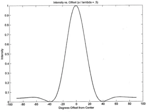
amplitude of the plane wave in the plane of the slit. Leaving aside intermediate steps, the following expression for the intensity as a function of 0, the angle from the center of the slit, is obtained after integrating and squaring equation 2.1:

1(6) = I0 sinc sin 1) (2.2)

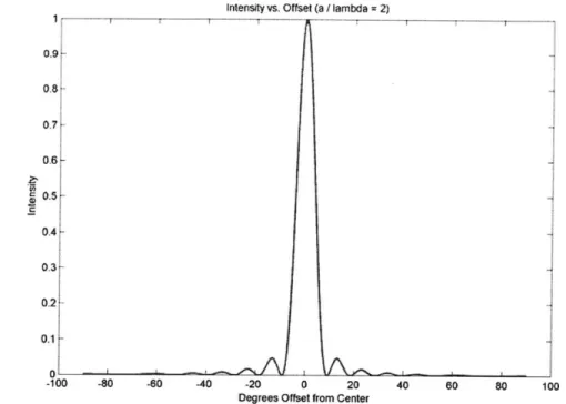
Where Io is a constant, and a is the width of the slit. Plotting this function for different values of a/A gives the following spatial profiles for different slits or element sizes.

Intensity vs. Offset (a I lambda = .5) 0.9 0.8 0.7 0.6 0. 5 0.4 0.3 02 0.1 100 -80 -40 -40 -20 0 20 40 80 80 10 Degrees Offset from Center

Figure 2: Intensity distribution for slit of width a =.5*)

Intensity vs. Offset (a /lambda = 1) 0.91 0~8 0.7' 0-6 04 03w 02 01 0 1--100 -80 -60 -40 -20 0 20 40 60 80 10 Degrees Offset from Center

Figure 3: Intensity distribution for slit of width a = X

0

Intensiy vs. Offset (a I lambda = 2)

-100 -80 -60 -40 -20 0 20

Degrees Offset from Center

1-0,9, 0.8 0.7 0.6 0.5 0.4 0.3 0.1

Figure 4: Intensity distribution for slit of width a = 2*A

N slit diffraction

Forgoing the derivation, it can be shown that for an array of N equally sized slits (or elements) with a center to center separation of d, the intensity profile as a function of offset angle from the center of the array (6), is the following (Ghatak):

a 2 sin(.d _2S

1(6) = sinc _I01 sin 0 L) d . (2.3)

A A sin si

0)1

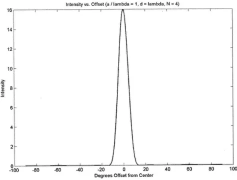
Plots for various values of d and N with a/A equal to 1 are shown below:

13

.4

Intensity vs. Offset (a / lambda = 1, d = lambda. N = 4) 14 " 10i-8 6 4 0 -100

Figure 5: Intensity distribution for 4 slits of width a = A spaced 1 wavelength apart

Intensity vs. Offset (a I lambda = 1, d = lambda, N = 16)

-80 -60 -40 -20 0 20 Degrees Offset from Center

40 60 80 100

Figure 6: Intensity distribution for 16 slits of width a = A spaced 1 wavelength apart

-80 -60 -40 -20 0 20 40 60 80 100

Degrees Offset from Center

300 250 200 150 100 5 0--100

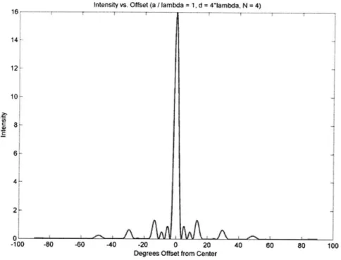
Intensity vs. Offset (a / lambda = 1. d 4*lambda. N = 4)

AJ

AI~AI1I

iv

-100 -80 -60 -40 -20 0 20 Degrees Offset from Center

4

~1

~1

60 80 100

Figure 7: Intensity distribution for 4 slits of width a = A spaced 4 wavelengths apart

Intensity vs. Offset (a / lambda - 1, d = 4*lambda, N = 16)

I fT I i I

I

k

I

A

.

-80 -60 -40 -20 0 20

Degrees Offset from Center 60 80 100

Figure 8: Intensity distribution for 16 slits of width a = A spaced 4 wavelengths apart

It is apparent that adding more elements further focuses the intensity spatially, as this effectively

increases the area of the array. Increasing element spacing also has the effect of further focusing the

15

~

AEA

101N

main beam, but this comes at the expense of increased energy in undesirable areas, called "side-lobes". This increased focusing ability is a large reason why arrays of this nature are useful.

Steering

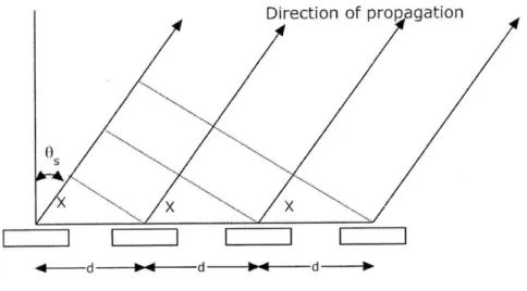
When a phase lag is added between successive elements, it becomes possible to adjust the intensity profile in a chosen direction. In order to determine the delay law between successive elements, and correspondingly find the phase difference between successive elements, it most useful to examine the geometry of the desired wavefront in terms of wave velocity, steering angle, and element spacing.

Direction of propagation

XX

4 1- d 10

Figure 9: Geometric view of beam steering

Using the geometry shown in Figure 9, where the lines without arrows represent the location of the desired constructive interference of the wavefront, the following expression for the distance x is geometrically obtained:

This represents the required distance between the peaks of adjacent transducers in order to steer in the direction 0s The distance x can then be written in terms of the required time delay by introducing the wave velocity and remembering that distance equals rate times time, resulting in:

ta d sin Os

tdel - d inO (2.5)

Finally, the time difference can be converted into a phase shift by utilizing the fact that:

tdel = 3' (2.6)

360'*f

Giving the following final expression for the phase shift (in degrees) between successive elements: 360'*f*d sin 0s (2.7)

C

Thus, for a given operating frequency, speed of sound, and element spacing it is possible to

determine the phase shift between elements to steer the wavefront of the array in a given direction.

Y

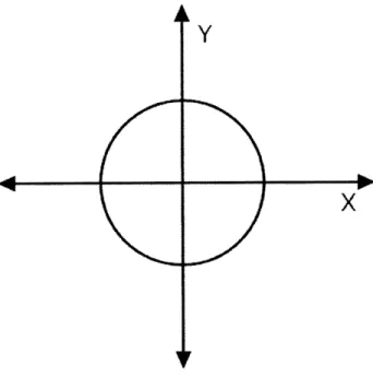
Figure 10: 2D Lens

In addition to steering the wavefront in a desired direction, it is also possible to develop delay laws, or relative phase shifts, that allow the intensity of the wavefront to peak at a desired distance from the array. This is accomplished using a parabolic phase shift akin to that of an optical lens. Observing that the phase transformation resulting from a 2 dimensional lens such as the one in Figure 10 can be written as shown in (2.8) (Goodman):

T(x, y) = exp (-j * (2 foa) * (x 2

+ y2)) (2.8)

Where focal is the focal point of the lens, and x and y are the coordinates at which the incoming wavefront encounters the lens. In order to apply this law to a 1 dimensional phased array, the y coordinate is set to zero, and the phase of a given element for a desired focusing distance is

calculated using the element's x coordinate as depicted in Figure 11. The resulting expression is shown in equation (2.9).

--Figure 11: Array with labeled X axis

Phase(n) = Lexp (-j * 2*ocaL) * (xi)) (2.9)

(2.9) results in a parabolic phase profile whose slope is determined by the desired focal distance.

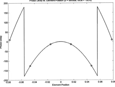
Example phase profiles for varying focusing distance for a six element array with elements spaced one wavelength apart and operating in air at 11 kHz (X=.0312cm) are shown below.

Phase Delay vs. Element Position (d lambda, focal 10cm) 200 150 100 50 0~ -0.06 -0.04 -0.02 0 0.02 0.04 0.06 Element Position

Figure 12: Phase profile for focusing at 10cm with A=3.12cm

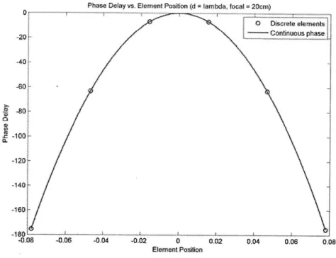
Phase Delay vs. Element Position (d lambda. focal 20cm) 0 Discrete elements -20Continuous phase -40 -80--100f -120 -140 -0.08 -0.06 -0.04 -0.02 0 0.02 0,04 0.06 0,08 Element Position

Figure 13: Phase profile for focusing at 20cm with X=3.12cm

Phase Delay vs. Element Position (d = lambda, focal = 40cm)

0 . . 0 Discrete elements Continuous phase A-5 -20 -301-.40 -80 -0.08 -0.06 -0.04 -0.02 0 0.02 0,04 0.06 0.08 Element Position

Figure 14: Phase profile for focusing at 40cm with A,=3.12

Note that the discontinuity in Figure 12 is the result of the phase delay wrapping around, i.e. a

phase delay of -190' is equivalent to a phase lead of 170'. As might be expected, for further focusing

distances the phase profile flattens out. To focus the array infinitely far away, all elements will be in phase.

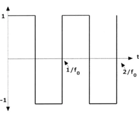
Filtering of Square Waves

t

10 2/f

Figure 15: Example square wave

The phased array system described within this thesis accomplishes the aforementioned steering and focusing calculations in the digital domain. As a result of having only two discrete output levels available for a single channel, it is only possible to generate shifted square waves. In order to drive the transducers at only the desired frequency, these square waves are filtered to suppress the undesired frequency components as much as possible. Using Fourier analysis, the frequency spectrum of the square wave at a frequency of fo shown in Figure 15 can be represented as follows (Weisstein):

f(X) = n=-3,s...-sin (n * 27r * t) (2.10)

All frequencies above the fundamental frequency fo are unwanted and must be filtered out. Luckily,

only odd harmonics are present and the amplitude of the higher order harmonics is already less than the amplitude of the fundamental. Therefore, the filtering requirements for removing these

harmonics are not too strict, and the chosen low pass filter easily suppresses the effects of the higher order harmonics.

Chapter 3

Software Interface

Overview

The focus of this chapter will be the software used to control the phased array. The chapter will begin with a description of the aspects of the array which can be adjusted and controlled in

software. Next, a description of the LabVIEW interface will be provided followed by an outline of the MATLAB script used by LabVIEW to generate the digital waveforms. This is followed by an

overview of the capabilities of the GP-24100 arbitrary waveform generator and a summary of the advantages and limitations of generating digital waveforms as the basis for a phased array as chosen for this project.

Overview of User Controls

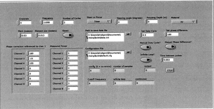
The following is a list of inputs available to the user of this system and a brief description of each. For reference, the user interface can be seen in Figure 16.

Channels The number of elements in the array.

Frequency The desired operating frequency of the array.

Cycles The number of cycles at the desired operating frequency that will be generated. In pulse mode this is the length of the pulse, in continuous mode this determines only the length of the waveform that is looped and should be set to a small number to increase the speed of waveform generation.

Pitch The center to center distance of the elements in the array. Element size The width of a single element in the array.

Phase correction Relative to element 1, the phase shift to apply to each channel in order to compensate for differences present in the analog portion of each

channel.

Measured power The measured output power of each channel at a 50 percent duty cycle. If desired, the software can compensate for differences in the analog amplification between channels by adjusting the duty cycle of the channels.

Steering angle The desired angle to steer the wavefront when in steering mode. Focusing depth The desired focal length when in focusing mode.

Steer or Focus Choose whether to steer or focus the wavefront.

Manual duty cycle Choose whether to manually set a duty cycle for all channels or if the duty cycle for each channel should be calculated from the measured powers.

Set duty cycle When in manual duty cycle mode, this value will be used for all channels.

Manual phase difference Choose whether to manually set a phase offset between successive channels or if the phase for each channel should be calculated from the

____________________desired steering angle or focusing depth.

Set phase difference When in manual phase difference mode, this will be used as the phase difference between adjacent channels.

Material Choose the material that the array will be operating in. This determines the speed of sound used in calculations.

Infinite loop Determines whether the generated waveform will be looped indefinitely or pulsed at a chosen interval.

Time between pulses Set the minimum time between pulses when in pulse mode. Note that the pulse rate is not well controlled and the time between pulses can vary, but will never fall below this value.

Configuration file path The location on the host PC of the configuration file for the GP-24100. Path to save data file The location on the host PC to save the data file containing the

generated waveform.

Sto When in pulse mode, this aborts operation. Reset When in continuous mode, this aborts operation.

Lab VIEW Interface

The purpose of the LabVIEW interface is to provide the user of the array with a front end which controls MATLAB scripts and Windows DLL calls to the GP-24100. LabVIEW is responsible for passing the user inputs along to the MATLAB script which will be described in the following section. After MATLAB has processed the input and produced the desired digital pattern, LabVIEW configures the GP-24100 using the supplied configuration file and user inputs by making DLL calls to application controlling the GP-24100. After the pattern is loaded onto the GP-24100, LabVIEW commands the device to begin outputting the loaded data using the supplied settings. For a detailed view of the LabVIEW block diagram, see Appendix B.

Generation of basic digital pattern

The generation of the digital waveform to be output to the GP-24100 is done using a MATLAB script. The first step to generating the desired digital square wave is to calculate the nominal time that a channel should be at the logic levels "high" or "low" for a single cycle at the desired operating frequency and a 50 percent duty cycle. This is done using the following simple formula.

Tonnom = TOffnom = n * .5 (3.1)

frequency

Next, this time must be converted into an equivalent number of digital samples (or clock cycles) at the GP-24100 clock frequency. The nominal samples on and off are calculated by dividing the desired time on and off by the time of a single sample and then rounding to obtain the nearest possible integer number of samples as follows:

Samples-onnom = round( Tonnom ) (3.2)

While any clock frequency up to 100MHz is possible, a higher clock frequency allows for increased precision, so it does not make sense to lower the operating clock. These values are used for

reference throughout pattern generation to ensure that all channels contain the same number of samples per cycle for arbitrary duty cycles.

Duty Cycle Calculation

To adjust for a difference in gain between channels in the analog portion of the signal processing chain, a technique has been developed to set the duty cycle of each channel such that the amplitude of the fundamental frequency at each channel is reduced to match the lowest measured amplitude. The amplitude of the fundamental frequency of a square wave of amplitude A and duty cycle D can be shown to be:

Amp = * (1 - cos(27rD)) (3.3)

A plot of the amplitude at the fundamental frequency versus duty cycle for can be seen in Figure 17,

as well as measured results for various duty cycles and the corresponding fundamental amplitude as reported by a digital oscilloscope. The input to filter curve represents the reported fundamental amplitude of a square wave with the corresponding duty cycle, and the output to fiber curve represents the reported fundamental amplitude after that square wave has been filtered to eliminate higher order harmonics.

Normalized Amplitudes vs. Duty Cycle _05 0.5-I E4 < 4 0.4-0.2 0.1 -0 0 1 02 0.3 0.4 0.5 0.6 07 0.8 0.9 1 Duty Cycle

Figure 17: Fundamental amplitude vs. duty cycle of square wave

Recognizing that the amplitude at the fundamental is a maximum for D equals .5, the channel with

the smallest measured amplitude is kept at a duty cycle of .5. The desired duty cycle for all other

channels is calculated by assuming the gain in the channel is a constant and then calculating the

value of D that will reduce the measured amplitude for that channel to the smallest measured

amplitude among all channels. The result is the following expression for the duty cycle of a channel:

D = 2r* Cos-(- (. 2026423673 * r2 *; Q ) (3.4)

Where Ad is the desired amplitude and Am is the measured amplitude for that channel. Using this it

is possible to digitally correct for gain mismatches between channels.

Generation of Individual Channels

With the duty cycle determined for each channel, whether it was calculated from measured amplitudes or input by the user, it is now possible to calculate the proper number of samples each

channel should be kept high and low. The technique is the same as in the general case, only now the times are adjusted using the determined duty cycle:

1 Ton = * D (3.5) frequency 1 Ton = * (1 - D) (3.6) frequency Ton Samples on = round(clock-period )(3.7)

Samples off = round(cToff )(3.8)

To create a full waveform for each channel, all that remains is to append the calculated number of ones and zeros in succession for the chosen number of cycles. With this done, the result is N channels consisting of square waves with varying duty cycles.

Generation of Full Digital Pattern

The final step is to apply a phase shift to the channels which need it, and to combine the channels into a single output file which can be read by the GP-24100. The phase shift for each channel is calculated based on the user's desired steering direction or focusing depth as described in the steering and focusing sections of Chapter 2, or taken from the manual phase shift input. Once a phase shift has been determined for each channel, the phase value is converted into a time delay, which is finally converted into a number of samples at the clock frequency using the following expression:

_si phase (39

tshift = 2nfrequency (3.9)

cycleshift = round( tshift

) (3.10)

Hard coded phase compensation is taken into account by using (3.9) and (3.10) to again convert phase into samples and then adding the two results to get the total samples to shift. The final step is to move the start of each channels pattern the proper number of samples, effectively changing the channels phase relative to where it began. Then the shifted channels are combined into a matrix which is written to a text file.

GP-24100

The relevant capabilities of the GP-24100 for this project are its 8 megabytes of embedded memory, 16 bits of data output, 6 bits of control output, and adjustable clock frequency up to 100MHz. The embedded memory creates a limit on the length of the pattern that can be loaded onto the device. The number of cycles this limit entails depends on the chosen operating frequency of the array as well as the clock frequency of the GP-24100. The 16 data bits limit the maximum number of channels the device can control to 16, and likewise the 6 control bits limit the number of switches or settings in the analog portion of the signal path that can be modified using the GP-24100 output.

The maximum clock frequency of 100MHz results in a limit on the phase precision between channels. The phase precision that can be obtained for a desired operating frequency can be found

by using the fact that the minimum time step that can be controlled with a 100MHz clock is:

Tperiod =

/100MHz

And the phase angle for a time delay is:

Phase = 3600 * frequency * tdelay (3.12)

As the frequency increases, the minimum phase step that can be commanded increases with it, reducing the precision of the array. See Figure 18 for a plot of minimum phase step compared to operating frequency.

Minimum Phase Step vs. Operating Frequency of Array

1

10"1

-103 10d 110

Operating Frequency

Figure 18: Minimum phase step as a function of operating frequency

&3 100 CD to CL E E₂₁₀ - -ORW-A06w

Chapter 4

Hardware

Overview

The analog hardware portion of this phased array consists of three subsections. The first is the low pass filter IC responsible for eliminating all undesirable higher order harmonics from the digital square wave output by the GP-24100. The second subsection is responsible for amplifying the filter output and driving the transducers which make up the array. Finally, there are a number of power management circuits which generate the power supply voltages needed to run the filters and amplifiers.

Low Pass Filtering

The low pass filter chosen for this project is the LTC6603 from Linear Technologies. This chip provides two channels which can operate in fully differential or single ended mode. It provides a 9th order low pass filter with a linear phase response along with an adjustable cut off frequency and gain. The schematic of the chip as utilized for this project is shown in Figure 19. What follows is a brief description of components and inputs which significantly alter the behavior of the IC as relevant to its use in this project. For a more detailed overview of the operation of this IC, see the datasheet provided by Linear Technology.

A

I

7

I

I

I~i

I

F-Wq .hane'

~

Figure 19: Schematic of low pass filter IC

Component Name Value

Cin .1uF

Ccm luF

Ccap .1uF

Rb 100k Ohm

T1 2N2222a

Table 2: Component values for filter

The value of the capacitors in this circuit are dictated by the datasheet and do not determine the behavior of the filter. The component which largely affects the operation of the filter is the resistance attached to the Rbias _{pin. This resistance controls the frequency of the filter's internal} clock according to the following relation:

fclk = 247.2MHz * 10k (4.1)

The clock frequency is then related to the cutoff frequency of the low pass filter according to equation (4.2):

fcutoff -

y

This holds true when the LPFO and LPF1 pins are at a logic level low. If LPFO is increased to a logic level high the cutoff frequency is increased by a factor of 4, and if LPF1 is increased to a logic level high the cutoff frequency is increased by a factor of 16. These effects are not cumulative, i.e. the largest active multiplier sets the cutoff frequency. The minimum high level voltage is 2 Volts and the maximum low level voltage is .8 Volts. Vcontrol2 and Vcontrol3 are provided by the control outputs of the GP-24100. In addition, Vcontroll is also supplied by the GP-24100 and provides a reduction of the resistance seen at the Rbias pin when set to high through the BJT switch, giving further control over the cutoff frequency.

Amplification

LT1221

V

Figure 20: Schematic of transducer driving amplifier

Component Name Value

Cin .1uF

Rin 100k Ohms

R1 3.3k Ohms

R2 470 Ohms

A schematic for the amplifiers which drive the array elements is shown in Error! Reference source not found.. The circuit utilizes an operational amplifier (op-amp) configured as a

non-inverting amplifier. The gain of this circuit depends on the values of R1 and R2 according to the following formula:

Gain = 1 + - (4.3)

Rz

The op-amp chosen for this circuit is the LT1221. It has a gain-bandwidth product of 150MHz. The gain in this configuration is 8 and this gain will therefore hold all the way up to 18MHz, well beyond the reasonable operating region of the digital portion of the array.

Power Circuitry

Three different supply voltages are required to power the filter and amplifiers. The amplifiers require +/- 14 Volts and the filter requires +3.5 Volts. The -14 Volts and +3.5 Volts are generated from an externally supplied +14 Volts.

The -14 Volts required to provide the amplifiers with a dual rail supply is generated using the LT1054 switched capacitor voltage converter.

'II

-144Vs

Figure 21: Schematic of voltage inverter

Component Name Value

Cin 2.2uF

Cout 1OOuF

Ccap 1O0uF

Rb 10k Ohms

T1 2n222

Table 4: Component values for voltage inverter

This IC is capable of providing up to 100mA of output current. The BJT transistor at the output is required to prevent the voltage at the Vout pin from being pulled up to a value above ground. Since this circuit exclusively powers the operational amplifiers in the system and the supply current in the op-amps flows from the positive supply voltage to the negative supply voltage, it is very likely that Vout could be charged to a positive value if the transistor were removed from the circuit.

The +3.5 Volts required to power the LTC6603 is generated using the LT1763 low dropout linear regulator.

+14

Volts

GND

+3.8

Volts

OUT

R 2

Figure 22: Schematic of filter power supply

Component Name Value

Cin 10uF

Cout 10uF

R1 261k Ohms

R2 124k Ohms

Table 5: Component values for filter power supply

The output voltage of this circuit is controlled via feedback to the ADJ pin. The output voltage can be adjusted from 1.22 Volts to 20 Volts according to the following formula:

Vout = 1.22V 1+ + Iadj * R1 (4.5)

RD

iadj = 30nA (4.6)

As indicated in the schematic, for the component value selected in this system Vout is equal to 3.8 Volts.

Chapter 5

Measurements

Test Setup

To examine the capabilities of the designed phased array, tests were run in an open air environment. Various steering and focusing profiles were chosen and a receiving piezoelectric transducer was used to measure the signal power at chosen spatial locations. In this way, a profile of the acoustic radiation pattern was determined for a given steering or focusing setting. In order to choose an operating frequency for the array in this environment, two frequency scans were

conducted. The first scan measured the power at the receiver over a range of with no signal present in order to determine the noise background. Next, the scan was repeated with the array

transmitting at max amplitude with all elements in phase at the frequency of interest in order to determine the signal level possible at that frequency. The two results can be seen in Figure 23.

Signal to Noise Rabo of Test Environment

Operating Frequency

Figure 23: Signal and noise comparison of test environment

11 KHz, the frequency with the highest signal level to noise level ratio, was chosen as the operating

frequency for the array in this environment. Note that at higher frequencies (above 50kHz) signal transmission is dominated by electromagnetic radiation rather than acoustic waves, making this test setup unsuitable for ultrasonic applications.

All of the following measurements were taken using an array of four elements of width

1.3cm spaced 3cm apart.

Beam steering results

The following figures depict the spatial radiation pattern at a distance of 38cm from the array. Data points were taken in the range from -22.5' to 22.50 with a step size of 2.5' between

successive measurements.

Received Power (normalized) vs. Receiver Offset (11kHz CW 0 degree transmitter offset)

- Theoretical 0 -E~ Mensured 0.8 0.7 0.8-0.4 0.3 -0.2 0.1 -30 -20 -10 0 10 20 30

Degrees Offset from Center

Received Power (normalized) vs. Offset from Center (Steering for -11 degrees) -25 -20 -15 -10 1'-0.9 0.8 0.7 0.6 0.5 0.4 0.3 0.2 0.1

Figure 25: Measured spatial radiation pattern for a 4 element array steered for -11 degrees

1 0.9 0.8 0.7 0.6 0.5 0.4 0.3 0.2 0.1 0--25

Received Power (normalized) vs. Offset from Center (Steering for -20 degrees)

-20 -15 -10 -5 0 5 10

Offset from Center (Degrees) 15 20

Figure 26: Measured spatial radiation pattern for a 4 element array steered for -20 degrees

These results show a clear ability to direct the radiation from the array in a preferred direction.

However, there is still some imprecision in the results that could stem from a number of factors.

-5 0 5 10 15 20 2

Offset from Center (Degrees)

---

_{4 e}

₀

The first factor is that the steering calculations are done using a fixed speed of sound, when in actuality the speed of sounds varies with air temperature and humidity. A 6% variation in the speed of sound (which is the equivalent of changing the air temperature from 900 Fahrenheit to 00

Fahrenheit) changes the steered angle by just over 10 Even more significant is the spacing between elements. If the elements are actually 2.8cm apart rather than 3cm, the steered angle changes by just over 1.50. The dependence of the steering on these factors, coupled with the difficulty in creating a perfectly regulated testing environment, help to explain the variation between the actual peaks and the desired location of the peak.

Beam focusing results

The following figures depict the received power at various distances from the array. Measurements were taken at distances in the range from 2cm to 25cm in front of the array, with a

step size of 1cm between measurements.

Received Power vs, Receiver Distance (11kHz CW) 0,05 No focusing 0.045- 0.04-o.035-L 0.031 0.025-0 _M I 0-015f 1 0.01 0.005 0 -- -5 15 20 25

Distance from Array (cm)

Received Power vs. Receiver Distance (11kHz CW) 0.03-0.025 0.02-0.015 0.01 0 5 10 15 20

Distance from Array (cm)

Figure 28: Received power vs. distance from array for focusing at 7cm

Received Power vs. Receiver Distance (11kHz CW)

0.02 5 -Z 0,015 0 0. -U E 0.01 10 15

Distance from Array (cm)

Figure 29: Received power vs. distance from array for focusing at 12cm

These results show a clear change in the intensity distribution from focusing attempts. However, they are subject to the same uncertainties as steering, namely variation in the speed of sound and

imprecision in the actual distance between elements. Furthermore, the results are affected by resonances created by adjusting the position of the receiver. When the receiver is very close to the

array and is at a distance near a multiple of the wavelength, a resonant cavity is created; skewing the results from what would be the ideal case with a non-interfering receiver.

Chapter 6

Conclusion

This thesis presented a phased array system capable of arbitrarily controlling the phase of up to 16 transducers. The shifted waveforms required to direct the array are generated digitally on a personal computer using LabVIEW and MATLAB. These waveforms are then output using the GP-24100, resulting in shifted square waves. Finally, the square waves are filtered and amplified before being applied to the transducers.

Measurements were conducted on a 4 element array operating in air at 11 KHz to demonstrate both steering and focusing of the array. Results clearly show that manipulating the preferred direction and focal distance of acoustic radiation is possible. Inaccuracy is evident in the results and is likely due to uncertainty regarding the precise speed of sound and the exact pitch of the array.

Possible improvements to this system include a more carefully manufactured structure to support the transducers, providing exactness in pitch calculations. Furthermore, the measurement process could be automated to provide finer resolution in data acquisition. In software, it should be possible to increase the capabilities of the array to include such features as steering and focusing at the same time. Hardware improvements could include amplifiers with increased gain for higher signal power, as well as adjustable gain for additional compensation if required.

Bibliography

Ajoy K. Ghatak, K. Thyagarajan. Optical electronics. Cambridge: Press Syndicate of the

University of Cambridge, 1989.

Bevan B. Baker, E. T. Copson. The Mathematical Theory of Huygens' Principle. New York: Chelsea Publishing Company, 1987.

Ghatak, Ajoy. Optics. New Delhi: Tata Mcgraw-Hill, 2005.

Goodman, Joseph W. Introduction to Fourier Optics. Greenwood Village: Roberts and Company Publishers, 2005.

S. Egusa, Z. Wang, N. Chocat, Z. M. Ruff, A. M. Stolyarov, D. Shemuly, F. Sorin, P. T. Rakich,

J.

Joannopoulos & Y. Fink. "Multimaterial piezoelectric fibres." Nature Materials (2010).

Walter Heywang, Karl Lubitz, Wolfram Wersing. Piezoelectricity: Evolution and Future of a Technology. Berlin: Springer, 2008.

Weisstein, Eric W. Fourier Series--Square Wave. 30 April 2010. 26 July 2010 <http://mathworld.wolfram.com/FourierSeriesSquareWave.html>.

Appendix A: MA

TLAB

Code

%TNPUTS FROM LAEVTEW: ath, steer, channels, f:eq, fcal, cycles, Pm, Pofl,

shift, fdcc, dcycle, 1 hard- no , sTpase, hardJphse, distnce,

ck freuency, max of 1 0

-clock freq 100e6;

clock-period 1 / clockfreq;

%define pattern a s emt v for now

pattern = [;

-norminal time on

Ton nom = (1 / freq) *.5;

nominal time off

Toff nom = (1 / freq) * .5;

%numb-er of samples to be on and oftf

samplesonInom = round(Tonnom/clockperiod); samplesoff nom = round(Toffnom/clock_period); %length of basic pattern

basic_length = samplesonnom + samples_off nom;

%generate duty cycle for each channel

%check if manual duty cycle is enable

if (dcycle > 0)

%if yes, set duty cycles from input

D(1:channels) = hard dcycle;

else

%otherwise look at lowest measured power and attempt to set all

%channels to that cower

Pg = min(Pm);

D = (1/(2*pi)) .* acos(1 - (.2026423673*pi^2 * Pg ./ Pm));

D = real(D);

end

%generate all channels

for t=l:channels

basic pattern = ;

%time while on for a given duty vcl

Ton = (1 / freq) * D(t);

%time while off for a gven d utv cycle

Toff = (1 / freq) * (1-D(t));

%n Umber of samples to be on or of f

samples on = round(Ton/clockperiod); samples-off = round(Toff/clock_period);

echeck

wl( (samples on + samples off) < basic-length + 1)

samples off = samples off + 1;

ena

%genra ept tern gin calclted a samle on and off pe c e

Seperate potions f the cycle (on and off)

pattern on = ones(l, samples-on);

pattern off = zeros(l, samples off)

for i=1:(2*cycles) if(mod(i,2) == 1)

basic pattern = [basic pattern pattern-on];

else

basic pattern = [basic pattern pattern off];

end

%h u rr en t channlO by amoun t equal to half the d f rence be tween

ampeson and samples on nm (or samples of:f and samp f

%this is to attempt to leave the phase unchanged after duty cylce mod ific~ati on

if(samples on < samples on nom)

dshift = (samples on nom - samples on) / 2;

shifty = basic pattern(basic length - abs(dshift):end);

basic pattern = [shifty basic pattern];

basic pattern = basic pattern(1:basic length);

end

if(samples off < samples off nom)

dshift = (samples off nom - samples-off) / 2;

shifty = basic pattern(basic length - abs(dshift):end);

basicpattern = [shifty basicpattern];

basic pattern = basic pattern(l:basic length);

ena

%append newly generated channe.l to toLa paLtern

pattern = [basicpattern' pattern];

end

%ene rate phase s.ift for e ctanne

%sLart by converting desired steering di rcion to radians

shift = pi * shift / 180;

waveletngth of sound

lambda = v sound/freq;

cho ses eth er sterin or Iocus 1ia or ow

if (steer == 1)

cphiase sh ft cal t a.~t i on fereach channe. (r aLtie a. channe )

cop- c-urrt channel o pattern 1

pattern_1 - pattern(:, (channels - 1))';

s'.check

chse

if(hard phase > 0)

Convrt hard phase of fset to radians and shi -ccording a to

curen channelasl

p = rem( ((setphase*l)*(pi / 180)), 2*pi);

else

scalculate Dhase to shift current channel in radians gi ven a direction to shl to and distance between elements

p = rem( (1*2*pi*distance*sin(shift) / lambda), 2*pi);

end

%equivalent time de'lav for calculated phase shift

ts = p / (2*pi*freq);

Slock

cycles to shift for given time delay

cshift = round( (ts) / clockperiod);

%a-py phase compensat ion

%clock cycles to shift for given phase correction

cc = round ( ((poff(1) * ( pi / 180) * (1 / (2 * pi * freq))) / clock_period) );

cshift = cc + cshift;

ocopy amount to shift from end of pattern, move to start, resize pattern to

%origi-nal length

if(cshift > 0)

shifty = pattern_l((length(basic_pattern) - abs(cshift)):end); pattern_1 = [shifty pattern_1];

pattern_1 = pattern_l(1:length(basicpattern)); end

%OR copy amount to shift from start of pattern, move to end, resize

%pattern to original length if(cshift < 0)

shifty = pattern l(1:abs(cshift)); pattern_l = [pattern_1 shifty];

pattern_1 = patternl((length(shifty) + 1):end); end

.replace current channel with shifted channel

pattern(:, (channels-1)) = patternl';

end

else

ecalau

k = (2*pi)/lambda;

a at eerpoints f each element in the aaray

a

arv sizer

array-width = distance*(channels - 1) + element-size;

pac.e centerpints properly

for n = 1:channels

centerpoints(n) = elementsize/2 + distance*(n-1);

%shift centerpoints to ce centered at zero

centerpoints = centerpoints - arraywidth/2;

%phase shCit fo each ca cu ated cnter p int and given f ocal length

phasef = angle(exp(-j*(k/(2*focal)).*centerpoints.^2));

timef phasef / (2*pi*freq);

%clock cycl es to shift for given tim delay

cshift = round( (timef) / clock-period);

%shi ft each channel the orocer amou

for l=1:channels

%copy current channel to patternIl

pattern_1 = pattern(:,(channels + 1 - 1))';

if(cshift(l) > 0)

shifty = pattern_l((length(basicpattern) - abs(cshift(l))):end);

pattern 1 = [shifty pattern_1];

pattern_1 = pattern_l(1:length(basicpattern));

end

%OR copy amlountr. so shi ft lfom sta rt C of pattern, move to end, resize

spattern

if(cshift(l) < 0)

shifty = pattern_l(1:abs(cshift(l)));

pattern_1 = [pattern_1 shifty];

pattern_1 = patternl((length(shifty) + 1):end);

end

replace current channel with shifted channel

pattern 1 = pattern l';

pattern(:, (channels + 1 -1)) = pattern_1;

end end

for y=channels:15

pattern fill = zeros(length(basic pattern), 1);

pattern = [pattern-fill pattern];

' PC' ) ;

Appendix B: LabVIEW Block Diagram

Inserts a time delay into the calling VI.

This Express VI is configured as follows: D,elay Time: 0.003 s