Imaging of structures in the high-latitude ionosphere: model comparisons

HAL Id: hal-00316429

https://hal.archives-ouvertes.fr/hal-00316429

Submitted on 1 Jan 1998

HAL is a multi-disciplinary open access

archive for the deposit and dissemination of sci-entific research documents, whether they are pub-lished or not. The documents may come from teaching and research institutions in France or abroad, or from public or private research centers.

L’archive ouverte pluridisciplinaire HAL, est destinée au dépôt et à la diffusion de documents scientifiques de niveau recherche, publiés ou non, émanant des établissements d’enseignement et de recherche français ou étrangers, des laboratoires publics ou privés.

Imaging of structures in the high-latitude ionosphere:

model comparisons

D. W. Idenden, R. J. Moffett, M. J. Williams, P. S. J. Spencer, L. Kersley

To cite this version:

D. W. Idenden, R. J. Moffett, M. J. Williams, P. S. J. Spencer, L. Kersley. Imaging of structures in the high-latitude ionosphere: model comparisons. Annales Geophysicae, European Geosciences Union, 1998, 16 (8), pp.969-973. �hal-00316429�

Imaging of structures in the high-latitude ionosphere:

model comparisons

D. W. Idenden1_{, R. J. Mo€ett}1_{, M. J. Williams}2_{, P. S. J. Spencer}2_{, L. Kersley}2

1_{School of Mathematics and Statistics, University of Sheeld, The Hicks Building, Sheeld, S3 7RH, UK} 2_{Department of Physics, University of Wales, Aberystwyth, SY23 3BZ, UK}

Received: 15 September 1997 / Revised: 10 April 1998 / Accepted: 14 April 1998

Abstract. The tomographic reconstruction technique generates a two-dimensional latitude versus height electron density distribution from sets of slant total electron content measurements (TEC) along ray paths between beacon satellites and ground-based radio receivers. In this note, the technique is applied to TEC values obtained from data simulated by the Sheeld/ UCL/SEL Coupled Thermosphere/Ionosphere/Model (CTIM). A comparison of the resulting reconstructed image with the `input' modelled data allows for veri®-cation of the reconstruction technique. All the features of the high-latitude ionosphere in the model data are reproduced well in the tomographic image. Reconstruct-ed vertical TEC values follow closely the modellReconstruct-ed values, with the F-layer maximum density (NmF2) agreeing generally within about 10%. The method has also been able successfully to reproduce underlying auroral-E ionisation over a restricted latitudinal range in part of the image. The height of the F2 peak is generally in agreement to within about the vertical image resolu-tion (25 km).

Key words. Ionosphere (modelling and forecasting; polar ionosphere) á Radio Science (instruments and

techniques)

1 Introduction

Signi®cant progress has been made since the early 1990s in the development of radio tomography as a new experimental technique for the study of the spatial distribution of the electron density in the ionised atmosphere (Kersley and Pryse, 1994). Independent veri®cation of the method has been obtained at auroral

latitudes from observations using the EISCAT incoher-ent scatter radar (Kersley et al., 1993; Walker et al., 1996). It is in the hostile environment of the highest latitudes that ionospheric tomography o€ers consider-able potential, with its ability to image spatial structures over a wide region from a limited number of ground stations. The present work reports results from a study of the use of tomography in the high-latitude ionosphere in which independent veri®cation has been obtained using the Sheeld/UCL/SEL Coupled Thermosphere/ Ionosphere/Model (Fuller-Rowell et al., 1996).

2 Ionospheric tomography

Ionospheric tomography uses radio signals from satel-lites received at a chain of stations approximately aligned in the sub-satellite track. Each receiver provides a sequence of measurements of total electron content (TEC) with a constant unknown o€set along the receiver-satellite ray path. Thus, a large number of relative TEC measurements along intersecting ray paths are obtained. These are inverted in a reconstruction algorithm to create a spatial image in two dimensions of the electron density. Transmissions from satellites in the former Navy Navigation Satellite System (NNSS) are used in ionsopheric tomography, these satellites being in near circular polar orbits at altitudes of about 1100 km. A number of di€erent reconstruction methods have been used in ionospheric tomography, with much e€ort directed to minimising the limitations imposed by the lack of horizontal ray paths in satellite-to-ground geometry.

The reconstruction technique for the present work uses a quadratic programming (QP) approach, (Spencer, 1998). QP methods involve solving linear equations such that a quadratic objective function relating the unknown is minimised. In the current application the constant TEC o€sets are eliminated by taking di€erences in TECs between neighbouring ray paths. Di€erence ray-path line integrals are then solved for a pixel-based representation

of the ionosphere, such that the electron density within each pixel is positive. Stable reconstructions are ensured by solving simultaneously for a continuous background ionosphere, de®ned by the linear sum of a number of functions derived from Chapman pro®les. By using the objective function to minimise the di€erence between the two representations, stable solutions are obtained over a range of peak heights and pro®le shapes. This technique also ensures physically realistic solutions, and produces absolute, not relative, electron densities.

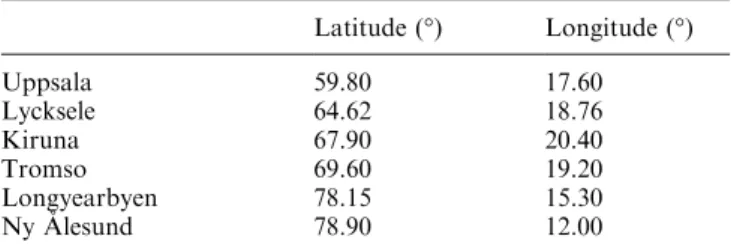
The receiver sites chosen for this simulation are the six locations in Scandinavia that have been used on a campaign basis by the Aberystwyth group for experi-mental studies of the high-latitude ionosphere using the tomographic method. The coordinates of the stations are listed in Table 1.

3 CTIM model description

The tomographic reconstruction technique was applied to slant TECs, with an unknown constant o€set, calculated from data obtained using results from the Sheeld/UCL/SEL Coupled Thermosphere/Iono-sphere/Model (CTIM) (Fuller-Rowell et al., 1996). It should be noted that relative, that is not absolute, TEC values form the input to the reconstruction algorithm used in the present study. Only the essential features of the CTIM model relevant to the present work are given here. More detailed descriptions can be found in the aforementioned reference. Model electron densities are calculated in the semi-Lagrangian (Fuller-Rowell et al., 1987; 1988) high-latitude ionosphere code that solves the coupled equations of continuity and momentum on straight `open' ®eld lines for the major species in the F-layer and topside, O+ _{and H}+_{, poleward of ‹35°}

latitude. The ®eld lines extend from an altitude of 100 km to 10 000 km and are ®xed in longitude and latitude, with separations of 18° and 2° respectively. In the present work, the input E ´ B, drifts and precipita-tion patterns come from the empirical models of Foster et al. (1986) and Fuller-Rowell and Evans (1987) respectively. These models are each parametrised by the hemisphere power index based on TIROS/NOAA precipitating particle measurements and are mutually consistent. The boundary conditions of chemical equi-librium at the bottom and zero ¯ux at the top of the ¯uxtable are imposed for the O+ _{ion. While chemical}

equilibrium at 100 km is also assumed for H+_{, account}

is taken of the polar wind by imposing an

empirically-based ¯ux at 10 000 km (Allen et al., 1986). The concentrations of the molecular ions, N2+, O2+ and

NO+_{, and the atomic ion N}+_{, are calculated by}

assuming chemical equilibrium. Ion temperatures are computed by solving the energy balance equation, which assumes that the rate at which heat is gained from the electron gas and by frictional heating is equal to the rate at which it is lost to the neutral air.

The thermospheric code solves the coupled momen-tum, continuity and energy equations by an explicit numerical scheme. Neutral temperatures, winds and densities are calculated on a global grid with the same horizontal resolution as the ionospheric code and with 15 ®xed pressure levels between altitudes of 80 km and 400 to 600 km depending on conditions. The calculation of coupling terms such as the ion drag force (Lorentz force), and Joule heating require ionospheric densities and conductivities. Poleward of ‹35° these are supplied by the high-latitude ionospheric code, Elsewhere the values are provided by the empirical model of Chiu (1975). Conversely, in the high-latitude code, calcula-tions of the heat exchange with the neutral gas, ion-neutral frictional heating, ®eld aligned ion-ion-neutral momentum transfer, and chemical production and loss rates require thermospheric temperatures, composition, densities, and winds. These parameters are provided by the thermospheric code. Thus, the thermospheric and ionospheric codes are fully coupled at high latitudes. 4 Model starting conditions and outputs

Model electron densities were calculated for the De-cember solstice (day 355) and convection and precipi-tation patterns keyed to a hemispheric power index of 6, corresponding to a KPof 3). The starting conditions for

the simulated satellite pass were obtained initially by running the model under steady-state conditions until the results become diurnally reproducible, which in this case was after four days. The simulated satellite pass began when the satellite was at latitude of 30° on the 15° meridian at 19:06 UT. The satellite was assumed to be travelling northwards in a polar orbit at an altitude of 1100 km, typical of the Navy Navigational Satellite System (NNSS) satellites used to obtain slant TECs experimentally. Model electron densities were integrated above 100 km along ray paths between the satellite and each receiving station (Table 1) from which the satellite would be visible. This set of slant TECs obtained from model data were written to a ®le of identical format to that obtained experimentally from a real satellite pass and used as input to the tomographic reconstruction algorithm. The path of the simulated satellite pass is shown in Fig. 1, superimposed on a contour plot of model NmF2 values at 19:18 UT, midway through the pass. Also shown are the positions of the northernmost and southernmost stations in the receiving chain.

The electron densities at the layer peak illustrate features that are characteristic of the high-latitude ionosphere in winter. The tongue of dayside ionisation from sunlit lower latitudes can be seen feeding into the

Table 1. Geographic coordinates of satellite receiving stations Latitude (°) Longitude (°) Uppsala 59.80 17.60 Lycksele 64.62 18.76 Kiruna 67.90 20.40 Tromso 69.60 19.20 Longyearbyen 78.15 15.30 Ny AÊlesund 78.90 12.00

polar cap in the post-noon sector. The polar hole is also clearly evident, where ¯ux tubes circulate in winter darkness trapped in the dawn convection cell, though the geometry of the present pass does not intersect this region. A narrow band of enhanced density can be seen at auroral latitudes in the evening sector, with a steep wall leading into the main trough on the equatorwards side also clearly visible.

5 Results

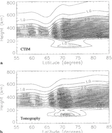
The tomographic reconstruction technique was applied to the data set of TEC values obtained from the model results as described. The modelled and reconstructed electron densities are shown as contour plots, in a latitude versus height plane, in Fig. 2a,b respectively. It can be seen that all of the major features are reproduced in the tomographic image. These can be most easily identi®ed by reference to the polar plot in Fig. 1. The tongue of ionisation feeding from the dayside across the polar cap in the convective ¯ow can be identi®ed with the maximum in the image at about 80°N latitude. The auroral zone, with a boundary blob surmounting the poleward wall of the trough, and underlying auroral-E layer can also be seen. The trough itself, with steep poleward wall and shallower gradient on the equator-ward side leading to the mid-latitude ionosphere, has also been reproduced in the image. The overall impres-sion gained from comparison of image and model is that the horizontal features are well replicated. In the vertical, the gradient of the bottomside appears

mar-ginally less steep than in the original, while the topside scale height di€ers slightly, causing the densities at the layer peak in the boundary blob and tongue of ionisation to be a little greater than those in the model. The tongue of ionisation, therefore, is a little less well-de®ned in the image.

More objective comparisons have been made in Fig. 3a±c, where the vertical TEC, the density at the layer peak (NmF2) and the height of the F2 peak (hmF2) are plotted as functions of latitude, for both modelled and reconstructed values. It can be seen that the tomographic technique gives vertical TEC values that are accurate to much better than 10% in general. This agreement is excellent bearing in mind that relative values of slant TEC were used as input to the reconstruction algorithm. The reconstructed NmF2 values show good agreement with the originals, but overestimate the densities in the trough minimum, and through the poleward wall leading to the boundary blob. By contrast, in the region of the tongue of ionisation the peak density in the image is some 10% below that of the model and it is in this region that the poorest agreement is found. The positions of the minimum and maximum associated with the trough are well within the one degree resolution of the model. The image was created on a 0.25° latitudinal grid. The values of hmF2 have been estimated using a curve-®tting technique through the pixels about the layer peak. The agreement is within ‹ one pixel height for both

Fig. 1. Northern Hemisphere polar contour plot of modelled winter solstice NmF2 values extending down to 40° latitude. Values on the bold contours are in units of 1010_m)3_{. Contours are separated by} 5 ´ 1010_m)3_{. The tick marks on the bold contours show the direction} in which NmF2 decreases. The dotted black line shows the simulated satellite path. Also shown are the positions of the southermost and northernmost receiving stations at Uppsala (U) and Ny AÊlesund (N)

respectively _{Fig. 2a, b. Contour plots of a modelled and b reconstructed electron} density distributions for the altitude/latitude slice below the simulated satellite track at 15°E longitude. Contour values are in units of 1010_m)3_{. The positions of the mid-latitude trough, the auroral region} and the polar cap tongue of ionisation can be identi®ed

reconstruction (25 km) and model (20 km) throughout the latitudinal range, though the image height exceeds that of the model everywhere apart from in the mid-latitude section. However, it can be noted that, apart from in the trough minimum itself, the form of the height change of the layer peak is followed in the image. A comparison of the vertical pro®le shapes from both model and image, at three latitudes, is shown in Fig. 4a± c. In general, there is very good treatment, though the densities in the high topside are consistently underesti-mated by a small amount throughout the entire latitu-dinal range of the reconstruction. At 60°N the peak density in the image is about 5% too large, though the peak heights show good agreement. Di€erences in the pro®les at 70°N can be attributed largely to the slight discrepancy in the peak height, though the tomographic technique has overestimated the peak density by a few percent. The auroral-E layer has been reproduced in the image, though its density is larger than in the model. At 80°N the main di€erence is in the density at the peak, though the discrepancy is still less than 10%.

6 Discussion

The work described has demonstrated that the tomo-graphic reconstruction technique is highly e€ective at

imaging ionospheric features at high latitudes. The method replicates well the horizontal structures in the ionisation, though the lack of horizontal ray paths in satellite-to-ground geometry results in greater uncer-tainty in the imaging of the vertical pro®le. The present results show that the quadratic programming method used here has been able to reproduce most of the essential features of the vertical structure of the ionisation, including the situation when there is an underlying auroral-E layer over only a limited latitudi-nal extent of the image. The discrepancies in the densities around the F2 layer peak are generally less than 10%, while di€erences in peak height are close to the limit set by the pixel resolution. The departures in pro®le shape in the high topside between model input and the reconstructed image can be attributed to the limitation imposed on the current work by the use in the quadratic programming method of only Chapman-type pro®les. Modi®cations to the method to incorporate a wider range of possible vertical ionospheric pro®les in the high topside could result in better agreement in that region. Improvements in the reproduction of the density at the peak of the layer would also be expected from this change. In essence, the tomographic method redistrib-utes the line integral of the density, the total electron content, throughout the pro®le, so that small

discrep-Fig. 3a±c. Comparisons of modelled (solid) and reconstructed (dotted) a vertical TEC (´ 1016_m)2_{), b (´ 10}11_m)3_{) NmF2 and c hmF2 (km)} values

Fig. 4a±c. Comparisons of modelled (solid lines) and reconstructed (dotted lines) altitude pro®les of electron density at latitudes of a 60°N, b 70°N and c 80°N

ancies in topside shape are compensated by more noticeable changes in peak density. While there are still improvements to be made, the present work shows that ionospheric tomography has advanced to a stage where it can yield reliable reproductions of the essential broad features of the high-latitude ionosphere.

Acknowledgements. The work was supported by PPARC awards GR/K06112 and GR/K98797 at Sheeld and Aberystwyth respectively. MJW acknowledges the support of PPARC research studentship.

Topical Editor D. Alcayde thanks D. Rees for his help in evaluating this paper.

References

Allen, B. T., G. J. Bailey, and R. J. Mo€ett, Ion distributions in the high-latitude topside ionosphere, Ann. Geophysicae, 4, 97, 1986. Chiu, Y.T., An improved phenomenological model of ionospheric

density, J. Atmos. Terr. Phys., 37, 1563, 1975.

Foster, J. C., J. M. Holt, R. G. Musgrove, and D. S. Evans, Ionspheric convection associated with discrete levels of particle precipitation, Geophys. Res. Lett., 13, 656, 1986.

Fuller-Rowell, T. J., and D. S. Evans, Height integrated Pederson and Hall conductivity patterns inferred from the TIROS-NOAA satellite data, J. Geophys. Res., 92, 7606, 1987.

Fuller-Rowell, T. J., D. Rees, S. Quegan, R. J. Mo€ett, and G. J. Bailey, Interactions between neutral thermospheric composition and the polar ionisation using a coupled ionosphere-thermo-sphere model, J. Geophys. Res., 92, 7744, 1987.

Fuller-Rowell, T. J., D. Rees, S. Quegan, R. J. Mo€ett, and G. J. Bailey, Simulations of the seasonal and universal time varia-tions of the thermosphere and ionosphere using a coupled, three-dimensional, global model, Pure Appl. Geophys., 127, 189, 1988.

Fuller-Rowell, T. J., D. Rees, S. Quegan, R. J. Mo€ett, M. V. Codrescu, and G. H. Millward, A coupled thermosphere-ionosphere model (CTIM), in STEP Handbook on Ionospheric Models, Ed. R. W. Schunk, 217, 1996.

Kersley, L., and S. E. Pryse, Development of experimental ionospheric tomography, Int. J. Imag. Syst. Tecn., 5, 141, 1994.

Kersley, L., J. A. T. Heaton, S. E. Pryse, and T. D. Raymund, Experimental ionospheric tomography with ionsonde input and EISCAT veri®cation, Ann. Geophysicae, 11, 1064, 1993. Spencer, P. S. J., A new solution to the problem of ionospheric

tomography using quadratic programming, Radio Sci. (in press), 1998.

Walker, I. K., J. A. T. Heaton, L. Kersley, C. N. Mitchell, S. E. Pryse, and M. J. Williams, EISCAT veri®cation in the devel-opment of ionospheric tomography, Ann. Geophysicae, 14, 1413, 1996.