Discovering and Reconciling Semantic
Conflicts: A Data Mining Perspective
Hongjun Lu, Weiguo Fan, Cheng Hian Goh, Stuart E. Madnick, David W. Cheung Sloan WP# 3957 CISL WP# 97-04
May 1997
The Sloan School of Management Massachusetts Institute of Technology
Discovering and Reconciling Semantic Conflicts: A
Data Mining Perspective
Hongjun Lu
Weiguo Fan
Cheng Hian Goh
Department of Information Systems & Computer Science
National University of Singapore
{luhj,fanweigu,gohch} @iscs.nus.sg
Stuart E. Madnick
David W. Cheung
Sloan School of Mgt
Dept of Computer Science
MIT
Hong Kong University
[email protected]
[email protected]
Abstract
Current approaches to semantic interoperability require human intervention in detect-ing potential conflicts and in defindetect-ing how those conflicts may be resolved. This is a major impedance to achieving "logical connectivity", especially when the number of disparate sources is large. In this paper, we demonstrate that the detection and reconciliation of semantic conflicts can be automated using tools and techniques developed by the data mining community. We describe a process for discovering such rules and illustrate the effectiveness of our approach with examples.
1 Introduction
A variety of online information sources and receivers (i.e., users and applications) has emerged at an unprecedented rate in the last few years, contributed in large part by the exponential growth of the Internet as well as advances in telecommunications technology. Nonetheless,
this increased physical connectivity (the ability to exchange bits and bytes) does not necessarily lead to logical connectivity (the ability to exchange information meaningfully). This problem is sometimes referred to as the need for semantic interoperability [6] among autonomous and heterogeneous systems.
Traditional approaches to achieving semantic interoperability can be identified as either tightly-coupled or loosely-coupled [5]. In tightly-coupled systems, semantic conflicts are iden-tified and reconciled a priori in one or more shared schema, against which all user queries are formulated. This is typically accomplished by the system integrator or DBA who is responsible for the integration project. In a loosely-coupled system, conflict detection and resolution is the responsibility of users, who must construct queries that take into account potential conflicts and identify operations needed to circumvent them. In general, conflict detection and recon-ciliation is known to be a difficult and tedious process since the semantics of data are usually present implicitly and often ambiguous. This problem poses even greater difficulty when the number of sources increases exponentially and when semantics of data in underlying sources changes over time.
It should be clear from the preceding discussion that automating the detection and recon-ciliation process will be an important step forward in achieving the intelligent integration of information. In this paper, we show how data mining techniques can be gainfully employed to this end. Our strategy consists of the application of statistical techniques to overlapping subsets of data present in disparate sources, through which rules for data conversion may be extracted. The remainder of this paper is organized as follows. Section 2 presents a scenario in which integrated access to heterogeneous information sources is required. We observed that when-ever information content in disparate sources overlap, we will have an opportunity for engaging in the automatic discovery of conflicts and their resolution. Section 3 presents a statistical ap-proach for conflict detection and resolution and introduces the supporting techniques. Section 4 presents details of three experiments which are used in illustrating and validating the approach taken. Finally, Section 5 summarizes our findings and describes the issues which need to be resolved in the near future.
LOCALDB:
hotel (hcode, location, breakfast, facilities, rate);
REMOTEDB:
hotel (hcode, state, breakfast, facilities, rate); tax-rate (state, tax-rate);
hotel tax-rate
hcode state meal bath rate state rate
1001 1 0 0 50 1 6
1002 2 1 1 80 2 10
1003 1 1 2 100 3 15
3001 1 1 0 120 4 18
Figure 1: Two example databases.
2 Motivational Example
Consider the scenario depicted in Figure 1. Both databases keep information about hotels, for which some are identical in both databases. For the purpose of this discussion, we assume that key-values used for identifying individual hotels are common to the two databases: e.g., the hotel with hcode 1001 in both LOCALDB and REMOTEDB refers to the same hotel.
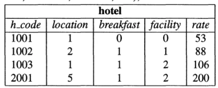
Observe however that although both databases have an attribute rate, different values are reported by the two databases even when the same real world entity is referenced. This anomaly arises from the fact that the two databases have different interpretation of rate: in the case of REMOTEDB, hotel rates are reported without taking applicable state taxes into consideration; on the other hand, hotel rates in LOCALDB are reported as charges "after-tax". Intuitively, we say that a semantic conflict exists between REMOTEDB and LOCALDB over attribute rate.
The meaningful exchange of information across different systems requires all semantic conflicts to be resolved. For instance, it would not be meaningful to write a query which com-pares hotel rates in REMOTEDB to those in LOCALDB without reconciling the conflict over attribute rate in the two databases. In the current example, this conflict can be resolved by
hotel
hcode location breakfast facility rate
1001 1 0 0 53
1002 2 1 1 88
1003 1 1 2 106
adding the tax-amount to the hotel rates reported in REMOTEDB. Notice that the computation of tax-value requires the multiplication of the hotel rates in REMOTEDB with a correspond-ing tax rate correspondcorrespond-ing to the state in which the hotel resides. We refer to the operation underlying the data transformation as a conversion function. Despite the critical role it plays in enabling semantic interoperability, the identification of appropriate conversion functions is a difficult task given that the assumptions underlying data representation are not always made explicit.
In general, conversion functions may take on various different forms. For example, it may be a lookup table which maps one string representation to another (e.g., "IBM" to "Interna-tional Business Machine"), or it may be any arbitrary "black-box" function (e.g., a dvips program which transforms a . dvi file to a . ps file). For our purpose in this paper, we con-sider only conversion functions which are arithmetic expressions. Although this represents only a subset of all possible conversion functions, arithmetic conversions are commonly en-countered in practise in a variety of different domains and are therefore important in their own right.
The remaining discussion will be presented using the relational data model without any loss of generality. For simplicity, we will use Horn clauses for representing conversion functions. For the example described earlier, we will write
L.hotel(hcode, state, breakfast, facilities, roomrate2)
-R.taxrate(state, taxrate), R.hotel(hcode, state, breakfast, facilities, roomratel), roomrate2 = (1 + 0.01 * tax-rate) * roomratel.
In the rest of this paper, we will demonstrate how conversion functions such as the one above can be discovered through the use of tools and techniques developed by the data mining com-munity.
3 A Statistical Approach for Conflict Detection and
Resolu-tion
Discovery of conversion functions proceeds in three steps. In Step 1 (semantic relevance anal-ysis), we use the techniques of correlation analysis to isolate attributes which are potentially semantically-related. In Step 2, we may rely on human intervention to identify attributes in
distinct databases which are to be treated as synonyms (even though these may embody se-mantic conflicts). Finally, in Step 3 (Quantitative Relationship Analysis), we apply regression analysis to generate the relevant conversion functions that allow values in one databases to be transformed to values that are meaning in a different context.
In the remainder of this section, we furnish the details of the statistical techniques employed in our approach.
3.1 Semantic Relevance Analysis
Given two sets of attributes from two databases, the objective of semantic relevance analysis is to find those attributes which either represent the same real world properties, or are derivable from each other. Such analysis can be conducted at two levels: at the metadata level or at the data level. In this study, we only discuss the second: i.e., we will attempt to isolate a subset of the attributes which are semantically-related by analyzing the data set, as opposed to relying on a thesaurus that tries to make sense of the attribute names (e.g., as in suggesting that attributes revenue and income are related).
If we view the attributes as variables, the problem we have on hand is similar to the problem of statistical correlation analysis. Given two variables, X and Y and their measurements (xi, Yi); i = 1, 2, .. ., n, we shall attempt to measure the strength of association between the two variables by means of a correlation coefficient r. The value of r is between -1 and +1 with r = 0 indicating the absence of any linear association between X and Y. Intuitively, larger values of r indicate a stronger association between the variables being examined. A value of r equal to -1 or 1 implies a perfect linear relation. While correlation analysis can reveal the strength of linear association, it is based on an assumption that X and Y are the only two variables under the study. If there are more than two variables, other variables may have some effects on the association between X and Y. Partial Correlation Analysis (PCA), is a technique that provides us with a single measure of linear association between two variables while adjusting for the linear effects of one or more additional variables. Properly used, partial correlation analysis can uncover spurious relationships, identify intervening variables, and detect hidden relationships that are present in a data set.
In our study, we use PCA to analyze the semantic relevance among attributes. Given two databases D1 and D2, we can treat the records in relations as measurements. Let R1 (Al, Al,..., Al) with primary key Al be a relation from D1, and R2 (A2, A2,... ,A2) with
primary key Al be a relation from D2. We also assume that two records r1 of R1 and r2of R2
refer to the same "real world" entity if rl.Al = r2.A2. Therefore, we can form measurements using records with the same key value from the two relations. Partial correlation analysis can be then applied to the data sets with (m + n - 2) variables (where m and n are the number of attributes in the two relations under investigation). The details of the various steps will be illustrated in next section.
Note that, correlation and semantic relevance are two different concepts. A person's height and weight may be highly correlated, but it is obvious that height and weight are different in their semantics. However, since semantic conflicts come from the difference in representation scheme and such representational difference is uniformly applied to each entity, high correla-tion should exist among the values of semantically related attributes. Correlacorrela-tion analysis can at least isolate the attributes which are likely to be related to one another for further analy-sis. In our approach exemplified in this paper, this step provides a preliminary clustering of semantically-related attributes which are then presented to respective user groups, who must now define the attributes which are to be treated as synonyms. Synonyms nonetheless may continue to embody semantic conflicts. When these conflicts can be resolved through arith-metic transformations, the underlying quantitative relationship can be uncovered automatically as described in the next section.
3.2
Quantitative Relationship Analysis
The discovery of quantitative laws from large data sets is a classic machine learning problem: to this date, various systems have been reported in the literature. Examples of these systems in-clude BACON [4], ABACUS [2] and COPER [3]. BACON, being one of the earliest systems, has made some interesting re-discoveries in physics and chemistry [4]. ABACUS improved upon BACON and is capable of discovering multiple laws [2]. In the case of COPER [3], phys-ical laws which can be modeled by a polynomial function can also be uncovered. A recently reported system, KEPLER [7], is an interactive system which is able to check data correctness and discover multiple equations. Another system, FORTY-NINER, borrows solutions from the early systems and adjusts them to the specific needs of database exploration [8].
One of the basic techniques for discovering quantitative laws is a statistical technique known as regression analysis. Thus, if we view the database attributes as variables, the re-lationships we are looking for among the attributes are nothing more than regression functions.
For example, the equation roomrate2 = (1 + 0.01 * tax_rate) * roomratel can be viewed as a regression function, where roomrate2 is the response (dependent) variable, tax_rate and room-ratel are predictor (independent) variables. In general, there are two steps in using regression analysis. First step is to define a model, which is a prototype of the function to be discovered. For example, a linear model of p independent variables can be expressed as follows:
Y = o +l3X + 2X2 +...3pXp +
where /3o,1 ,..., l3p are model parameters, or regression coefficients, and p is an unknown random variable that measures the departure of Y from exact dependence on the p predictor
variables.
With a defined model, the second step in regression analysis is to estimate the model param-eters i1, ... , l3p. Various techniques have been developed for the task. The essence of these
techniques is to fit all data points to the regression function by determining the coefficients. The goodness of the discovered function with respect to the given data is usually measured by the coefficient of determination, or R2. The value R2 ranges between 0 and 1. A value of 1 implies perfect fit of all data points with the function.
In our experiments reported in the next section, regression analysis is used primarily to discover the quantitative relationships among semantically-related attributes. One essential difference between the problem of discovering conversion functions and the classic problem of discovering quantitative laws is the nature of the data. Data from experimental results from which quantitative laws are to be discovered contains various error, such as measurement er-rors. On the other hand, semantic conflicts we are dealt with are due to different representations which are uniformly applied to all entities, the discovered function that resolves the conflicts should apply to all records. If the database contains no erroneous entries, the discovered func-tion should perfectly cover the data set. In other words, funcfunc-tions discovered using regression
analysis should have R2 = 1.
In some instances, the R2 value for a regression function discovered may not be 1. For example, this may be the case when the cluster does not contain all attributes required to solve the conflicts; in which case, no perfect quantitative relationship can be discovered at all. More-over, it is also possible that the conflicts cannot be reconciled using a single function, but are reconcilable using a suitable collection of different functions. To accommodate for this
pos-hcode location breakfast facility L.rate meal bath R.rate taxrate
1001 1 0 0 53 0 0 50 6
1002 2 1 1 88 1 1 80 10
1003 1 1 2 106 1 2 100 6
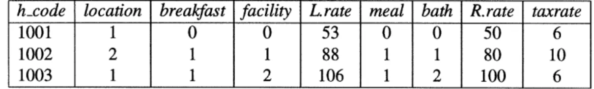
Figure 2: The relation obtained by joining relations in REMOTEDB and LOCALDB. sibility, we extend the procedure by partitioning the data set (whenever a suitable regression function cannot be found) and attempting to identify appropriate regression function for each of the partition taken one at a time. This partitioning can be done in a number of different ways. For our purpose, we use the simple heuristic of partitioning the data set using categorical at-tributes present in a relation. The rationale is, if multiple functions exist for different partitions of data, data records in the same partition must have some common property, which is most likely reflected by values assumed by some attributes within the databases being investigated.
4 Automatic Discovery of Conversion Functions
To provide a concrete illustration of this approach proposed in the preceding section, we de-scribe below three experiments. The first two are based on the scenario introduced in the motivational example; the last presents a simplified version of a real example which we have encountered.
4.1 Experiment One
We shall consider the databases REMOTEDB and LOCALDB as shown earlier. Since hotel and taxrate are in the same database, we assume that they do not have any conflicts on the attribute state. To simplify the ensuing discussion, we shall assume that these two tables are "joined" to yield the relation shown in Figure 2; the attribute rate in LOCALDB and REMOT-EDB are prefixed with L and R respectively to avoid any ambiguity. The attributes in this relation will be used as inputs to Step 1 of our procedure and serve as the basis for identifying attributes which are semantically-related. For simplicity, we shall also ignore attributes meal and bath in the joined database since they have the same value as breakfast andfacility.
Table 1: Domain values used in materializing the synthetic databases. attribute state taxrate facility breakfast R.roomrate values 0-40 1-18 {0, 1, 2} {0, 1} 20-500
semantic knowledge in the form of conversion functions, we created the synthetic databases corresponding to LOCALDB and REMOTEDB. This is accomplished by generating the values of the attributes identified earlier using a uniform distribution, according to Table 1. Values of L.roomrate are generated using the following formula:
L.roomrate = (1 + 0.01 * taxrate) * R.roomrate The number of tuples in the dataset is 1000.
We now present detailed descriptions of the three steps corresponding to our strategy.
1. Identifying semantically related attributes
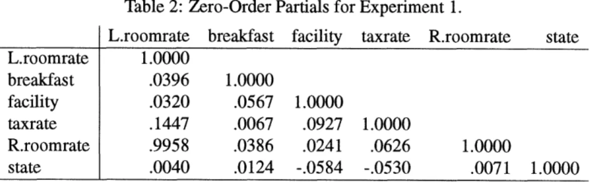
To identify attributes which may be semantically-related, a partial correlation analysis is performed on the dataset. Table 2 lists the result.
Table 2: Zero-Order Partials for Experiment 1.
L.roomrate breakfast facility taxrate R.roomrate state L.roomrate 1.0000 breakfast .0396 1.0000 facility .0320 .0567 1.0000 taxrate .1447 .0067 .0927 1.0000 R.roomrate .9958 .0386 .0241 .0626 1.0000 state .0040 .0124 -. 0584 -. 0530 .0071 1.0000
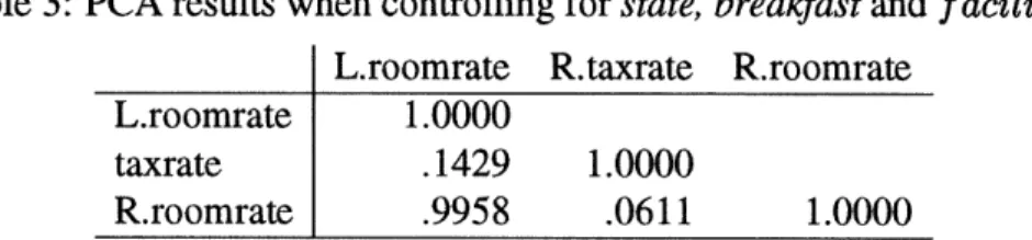
It can be seen that if 0.1 is chosen as a threshold, L.roomrate, taxrate, and R. roomrate will be considered to be correlated. To verify this, we further perform a PCA analysis while controlling for the other three attributes, i.e. state, breakfast, and facility. Table 3 shows the result of analysis:
Table 3: PCA results when controlling for state,
L.roomrate R.taxrate R.roomrate L.roomrate 1.0000
taxrate .1429 1.0000
R.roomrate .9958 .0611 1.0000
We can see from Table 3 that L. roomrate and R. roomrate indeed have a very strong linear relationship. But the relationship between L.roomrate and R.taxrate is not so obvious (0.1447). To further determine whether L.roomrate and R.taxrate are correlated, we make another partial correlation analysis between them by controlling R.roomrate. The result is shown below in Table 4:
Table 4: PCA results when controlling for R. roomrate. L.roomrate R.taxrate
L.roomrate 1.0000
taxrate .8975 1.0000
This result indicates that L.roomrate does correlated highly with taxrate. We there-fore conclude that attribute L.roomrate is highly related to two attributes, taxrate and R.roomrate, in the remote database.
2. Defining the synonyms
From a user or application perspective, certain attributes present in different databases may be treated as synonyms. Thus the rate attribute in both LOCALDB and REMOT-EDB are treated as synonyms (having the same meaning). Notice that they two attributes may or may not be identical syntactic tokens: i.e., having the same attribute name (al-though they happen to be the same in this instance). Furthermore, two attributes may be viewed as synonyms by one user and are yet semantically distinct from another user's viewpoint. Hence, a knowledgeable user may understand the semantic disparity between hotel rates reported in REMOTEDB and LOCALDB and therefore choose to treat the two attributes as different. For this reason, it is mandatory for synonyms are to be
fined by users depending on their understanding. This however does not mean that users will have to peruse through the thousands of attributes which are present in disparate databases. Clearly, the attributes which have been identified in Step 1 above serve as a useful starting point whereby potential synonyms can be identified.
Notice that there is no right or wrong synonyms. If two attributes are identified as syn-onyms, they will be used as input to the next step in the discovery process in which an attempt is made to identify the relationship between the two. Two attributes which are semantically-related in some way may however not be labeled as synonyms. For instance, the attribute rate could have been treated as distinct in REMOTEDB and LO-CALDB. This however will not pose any problem so long as the user do not attempt to compare them under the assumption that they are referring to the same thing.
3. Discovering the relationship
The final step in our process is to find the quantitative relationship among attributes which are identified as synonyms. For the example at hand, we need to find the re-lationship among L.roomrate, taxrate and R.roomrate, assuming that L.roomrate and R.roomrate are identified as synonyms.
To perform the regression analysis, we choose one of the synonyms as the dependent variable. Suppose L.roomrate is chosen for this purpose, with taxrate and R. roomrate as independent variables. Since we have two independent variables, a multiple regression model is used. Let Y denote L.roomrate, x1 and x2 denote taxrate and R.roomrate
respectively. The regression analysis is to find the coefficients, /i3, 1 < i < 3 of the following model:
Y = fPlx + 32X + 33XX 1X2 + (1) By applying the multiple regression analysis to the given dataset, we obtain the following result:
P1 = -4.61989E-14
p/3 = 0.010000
e = 0.000000
Since 31 is negligible, we obtain the following by substituting the variables with the original attribute names:
L.roomrate = R.roomrate + 0.01 * taxrate * R.roomrate (2) The preceding result can be rewritten into the following Horn clause
L.hotel(hcode, state, breakfast, facilities, roomrate2)
+-R.tax(state, taxrate), R.hotel(hcode, state, breakfast, facilities, roomratel), roomrate2 = (1 + 0.01 * taxrate) * roomratel.
which is what we have used in creating the synthetic databases for this experiment.
4.2 Experiment Two
In this experiment, we modified the test data set by deleting the attribute taxrate. In other words, we have a data set of 1,000 tuples, comprising of the attributes: (hcode, state, L. roomrate, breakfast, facility, R. roomrate).
1. Identifying semantically-related attributes & define synonyms
Similar to what described in the previous experiment, we concluded from the partial correlation analysis that L.roomrate is highly correlated to R.roomrate. As before, the user may choose to treat L.roomrate and R.roomrate as synonyms. This prompts us to proceed on with the next step.
2. Discovering the relationships
Applying the regression analysis to the data set, we obtained the following:
where the coefficient of determination R2 = 0.99123. 3. Partitioning the data set
Since R2 is not equal to one, we may suspect that the equation obtained does not
rep-resent the true relationship among the attributes. (A high-value for R2 may however be acceptable if the values are known to be "noisy".) One approach for circumventing this problem is to partition the data set so that a more "consistent" relationship can be identi-fied. For this purpose, we note that there are three categorical attributes: state, breakfast, and facility, with 40, 2, and 3 distinct values respectively. Consequently, we partition the dataset according to each of the three attributes in turn and regression analysis was
applied to each partition. The results can be summarized as follows: * Partitioning based on state
Since there are 40 distinct values in the dataset, 1000 tuples were partitioned into 40 partitions. For each partition, regression analysis was applied. We obtained the following results:
State Equation discovered R2 0 L.roomrate = 1.00 * R.roomrate 1
1 L.roomrate = 1.09 * R.roomrate 1 ..
38 L.roomrate = 1.08 * R.roomrate 1
49 L.roomrate = 1.04 * R.roomrate 1
* Partitioning based on breakfast
There are 2 distinct values for breakfast in the data set, 1000 tuples were partitioned into 2 partitions. The result of regression analysis is as follows:
Breakfast Equation discovered R2
1 L.roomrate = 1.06 * R.roomrate - 0.133591 0.99189 2 L.roomrate = 1.07 * R.roomrate - 1.724193 0.99121
* Partitioning based on facility
There are 3 distinct values for facility in the data set, 1000 tuples were partitioned into 3 partitions. The result of regression analysis is as follows:
Facility Equation discovered R2
1 L.roomrate = 1.066 * R.roomrate - 1.702022 0.99235 2 L.roomrate = 1.058 * R.roomrate + 0708756 0.99187 3 L.roomrate = 1.076 * R.roomrate - 1.728803 0.99070
It is obvious that state is the best choice for achieving a partitioning that yields a consis-tent relationship.
From the equation that is discovered, we can create a new relation, called ratio, which reports the tax-rate for each of the 40 states:
ratio(0, 1.00). ratio(l, 1.09).
ratio(38, 1.08). ratio(39, 1.04).
This in turn allows us to write the conversion rules:
L.hotel(hcode, state, breakfast, facilities, roomrate2) +
ratio(state, ratio), R.hotel(hcode, state, breakfast, facilities, roomratel), roomrate2 = 1 + ratio * roomratel.
4.3 Experiment Three
In this final experiment, we created two synthetic relations which are presumably obtained from two distinct sources:
stock (scode, currency, volume, high, low, close); stkrpt (scode, price, volume, value);
Relation stk rpt is derived from the source relation stock. For this experiment, we generated 500 tuples. The domain of the attributes are listed in the following table, together with their variable names used in the analysis.
Variable Relation Attribute Value Range X1 stock, stkrpt scode [1, 500]
X2 stkrpt price stock.close*exchange-rate[stock.currency] X3 stkrpt volume stock.volume * 1000
X4 stkrpt value stkrpt.price * stk rpt.volume X5 stock currency 1, 2, 3, 4, 5
X6 stock volume 20-500
X7 stock high [stock.close, 1.2*stock.close] X8 stock low [0.85*stock.close, stock.close]
X9 stock close [0.50, 100]
It can be seen that, there are rather complex relationship among the attributes. We proceed with conflict detection and reconciliation as before.
1. Identifying correlated attributes
The zero-order partial correlation analysis on the data set gave the result as shown below:
X3 X4 1.0000 .3243 -. 0645 1.0000 -. 0307 -. 0309 -. 0349 1.0000 .5416 .3243 .3331 .3318 .3357 X5 1.0000 -. 0645 -. 0245 -. 0217 -. 0193 X6 1.0000 -.0307 -. 0309 -. 0349 X7 X8 X9 1.0000 .9905 .9946 1.0000 .9959 1.0000 X1 1.0000 .0508 -. 0829 .0425 -. 0311 -. 0829 .0762 .0661 .0725 X1 X2 X3 X4 X5 X6 X7 X8 X9 X2 1.0000 -. 0607 .7968 .6571 -. 0607 .4277 .4355 .4397
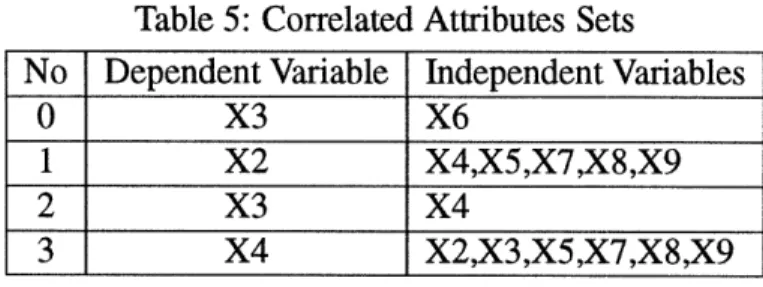
Using 0. 1 as the threshold value and treating variables representing attributes from stkrpt as the dependent variables, we identify the following correlated variable sets:
_ _
----Table 5: Correlated Attributes Sets
No Dependent Variable Independent Variables
0 X3 X6
1 X2 X4,X5,X7,X8,X9
2 X3 X4
3 X4 X2,X3,X5,X7,X8,X9
2. Discovering relationships among related attributes
Each correlated attribute set was analyzed using regression analysis to discover the rela-tionships.
* SetO
Since the coefficient of X3 and X6 is 1 and the values of X3 are not equal to that of X6, linear regression analysis was conducted on these two variables. The following result was obtained:
X3 = 1000 * X6 (4)
This is consistent with the semantics of data used in creating the synthetic databases. * Set
A brute force method is to use the following model which consider all one and two variable terms: X2 = B1*X4+B2*X5+B3*X7 (5) + B4*X8+B5*X9 + B6*X4*X5+B7*X4*X7 + B8*X4*X8+B9*X4*X9 + B10*X5*X7+Bll*X5*X8 + B12*X5*X9
The following regression equation was obtained with R2 = 0.90602:
X2 = 1.2762 * X5 + 1.6498 * X7 + 1.0075 * X8 (6) - 2.0270 * X9 - 2.4475 * X5 * X7
- 0.5275 * X5 * X8 + 3.8573 * X5 * X9
Since the the coefficient of determination R2
#
1, we partitioned the data according to the only categorical variable X5. Since X5 has five distinct values, the 500 tuples were partitioned into 5 partitions. Furthermore, the result of model 5 reveals that coefficients B1,B6,B7,B8, and B9 are zero. We can construct for each partition asimpler model
X2 = B3*X7+B4*X8+B5*X9 (7)
The regression results are given below:
X5 equation discovered R2 0 X2 = 0.4 * X9 1 1 X2 = 0.7 * X9 1 2 X2 = 1.0 * X9 1 3 X2 = 1.8 * X9 1 4 X2 = 5.8 * X9 1
In fact, the coefficient shown in Table 2 are the exchange rates used in generat-ing stkrpt.price from stock.close based on stock.currency. The regression analysis correctly discovered this fact automatically.
* Set 2:
As the R2 value of the regression analysis on the whole data set is not equal to 1, we repeat the regression analysis after partitioning the data set based on X5. The results are as follows:
Data Set X5 Equation Discovered R2 nonpartitioned all X3 = 0.0012 * X4 + 232938.0964 0.10517 partition 0 X3 = 0.2005 * X4 + 163787.2507 0.37291 1 X3 = 0.1259 * X4 + 154285.2230 0.41848 2 X3 = 0.0068 * X4 + 180850.1938 0.38318 3 X3 = 0.0054 * X4 + 144068.7345 0.35892 4 X3 = 0.0016 * X4 + 126240.6993 0.50320
In both instances, no consistent relationship is found. * Set3:
The regression analysis on set 4 yields the following result:
X4 = X2 * X3 (8)
with R2 = 1.
The above results can now be summarized in the following conversion rule: stkpt(scode, price, volume2, value)
-stock(scode, currency, volumel, , , close), exchange(currency, rate), volume2 = 1000 * volumel, price = close * rate, value = price * volume2.
exchange(0, 0.4). exchange(l, 0.7). exchange(2, 1.0). exchange(3, 1.8). exchange(4, 5.8).
where exchange is a new relation with two attributes (currency, rate), in which rate is presumably the exchange-rate for converting other currencies into the currency used in stkrpt.
5 Conclusion
The quest for semantic interoperability among autonomous and heterogeneous information systems has led to a proliferation of prototypes. However, as far as we know, no one has yet done any work on the automatic detection and discovery of semantic conflicts. In this paper, we have presented the motivation for this problem, and have demonstrated how conflict detection and resolution can be mostly automated using various statistical techniques. We also presented three experiments in which the techniques are applied to uncover hidden relationships between data elements. While it is clear that we have only addressed a small subset of the problems, we are convinced that the work reported here remains significant for the role it plays in breaking the ground for an important class of problems.
The astute reader may object to the approach proposed in this paper by pointing out that the statistical techniques are expensive and cannot be used to support ad hoc queries at real-time. Our response is that it is never our intention to apply the regression methods at real-time. On the other hand, data analysis should be performed off-line and at the time when a new system is brought into the "federation" of inter-operating systems. The rules which are discovered during this process can be used as input to the definition of a shared schema where the conflicts are being resolved. In loosely-coupled systems where shared schemas are not defined a priori, the rules may be stored as part of a user's profile which can be drawn upon (as part of the local knowledge base) whenever a query is to be formulated.
We are currently examining extensions to this work that will allow it to be incorporated into a Context Interchange System [1]. The key observation here is that the extraction of the conversion function alone is not sufficient, and that further work is needed to be able to also uncover the meta-data that is associated with different information sources. For example, in the case of Experiment 2, it is not good enough to identify the ratios (state-tax) that are needed for computing the tax-value: it would have been more valuable if we are able to match the ratios to yet another data source furnishing the state-tax percentage and figure out instead that different hotels have different tax rates by virtue of its location. Thus, if we know indeed that all hotels reported in a given database have a uniform tax rate of 6%, we might formulate a hypothesis that these are all hotels located in Massachusetts. In principle, these conclusions can be derived using the same statistical techniques as those which we have described. Further work however remains necessary to verify their efficiency.
References
[1] BRESSAN, S., FYNN, K., GOH, C., JAKOBISIAK, M., HUSSEIN, K., KON, H., LEE, T.,
MADNICK, S., PENA, T., Qu, J., SHUM, A., AND SIEGEL, M. The COntext INterchange mediator prototype. In Proc. ACM SIGMOD/PODS Joint Conference (Tuczon, AZ, 1997). To appear.
[2] FALKENHAINER, B., AND MICHALSKI, R. Integrating quantitative and qualitative dis-covery: The abacus system. Machine Learning 4, 1 (1986), 367-401.
[3] KOKAR, M. Determining arguments of invariant functional description. Machine Learning
4, 1 (1986), 403-422.
[4] LANGLEY, P., SIMON, H., G.BRADSHAW, AND ZYTKOW, M. Scientific
Discovery: An
Account of the Creative Processes. MIT Press, 1987.
[5] SCHEUERMANN, P., YU, C., ELMAGARMID, A., GARCIA-MOLINA, H., MANOLA, F.,
MCLEOD, D., ROSENTHAL, A., AND TEMPLETON, M. Report on the workshop on
heterogeneous database systems. ACM SIGMOD RECORD 4, 19 (Dec 1990), 23-31. Held at Northwestern University, Evanston, Illinois, Dec 11-13, 1989. Sponsored by NSE [6] SHETH, A., AND LARSON, J. Federated database systems for managing distributed,
het-erogeneous, and autonomous databases. ACM Computing Surveys 3, 22 (1990), 183-236. [7] WU, Y., AND WANG, S. Discovering functional relationships from observational data. In
Knowledge Discovery in Databases (The AAAI Press, 1991).
[8] ZYTKOW, J., AND BAKER, J. Interactive mining of regularities in databases. In Knowl-edge Discovery in Databases (The AAAI Press, 1991).