HAL Id: hal-00316936
https://hal.archives-ouvertes.fr/hal-00316936
Submitted on 1 Jan 2001
HAL is a multi-disciplinary open access
archive for the deposit and dissemination of
sci-entific research documents, whether they are
pub-lished or not. The documents may come from
teaching and research institutions in France or
abroad, or from public or private research centers.
L’archive ouverte pluridisciplinaire HAL, est
destinée au dépôt et à la diffusion de documents
scientifiques de niveau recherche, publiés ou non,
émanant des établissements d’enseignement et de
recherche français ou étrangers, des laboratoires
publics ou privés.
Cluster magnetic field observations in the
magnetosheath: four-point measurements of mirror
structures
E. A. Lucek, M. W. Dunlop, T. S. Horbury, A. Balogh, P. Brown, P. Cargill,
C. Carr, K.-H. Fornaçon, E. Georgescu, T. Oddy
To cite this version:
E. A. Lucek, M. W. Dunlop, T. S. Horbury, A. Balogh, P. Brown, et al.. Cluster magnetic field
obser-vations in the magnetosheath: four-point measurements of mirror structures. Annales Geophysicae,
European Geosciences Union, 2001, 19 (10/12), pp.1421-1428. �hal-00316936�
Annales
Geophysicae
Cluster magnetic field observations in the magnetosheath:
four-point measurements of mirror structures
E. A. Lucek1, M. W. Dunlop1, T. S. Horbury1, A. Balogh1, P. Brown1, P. Cargill1, C. Carr1, K. -H. Fornacon2, E. Georgescu3,4, and T. Oddy1
1Space and Atmospheric Physics, The Blackett Laboratory, Imperial College, London, UK 2Institut f¨ur Geophysik und Meteorologie, Technische Universit¨at Braunschweig, Germany 3Max-Planck-Institut f¨ur extraterrestrische Physik, Garching, Germany
4Institut of Space Sciences, Bucharest, Romania
Received: 21 March 2001 – Revised: 20 June 2001 – Accepted: 27 June 2001
Abstract. The Cluster spacecraft have returned the first
si-multaneous four-point measurements of the magnetosheath. We present an analysis of data recorded on 10 Novem-ber 2000, when the four spacecrafts observed an interval of strong mirror-like activity. Correlation analysis between spacecraft pairs is used to examine the scale size of the mir-ror structures in three dimensions. Two examples are pre-sented which suggest that the scale size of mirror structures is
∼1500–3000 km along the flow direction, and shortest along the magnetopause normal (< 600 km), which, in this case, is approximately perpendicular to both the mean magnetic field and the magnetosheath flow vector. Variations on scales of
∼750–1000 km are found along the maximum variance di-rection. The level of correlation in this direction, however, and the time lag observed, are found to be variable. These first results suggest that variations occur on scales of the or-der of the spacecraft separation (∼ 1000 km) in at least two directions, but analysis of further examples and a statistical survey of structures observed with different magnetic field orientations and tetrahedral configurations will enable us to describe more fully the size and orientation of mirror struc-tures.
Key words. Magnetosphenic physics (magnetosheath; plasma waves and instabilities)
1 Introduction
Magnetosheath waves have previously been studied using both single (e.g. Anderson et al., 1994; Lacombe et al., 1995; Lucek et al., 1999) and more rarely dual spacecraft data (Tsu-rutani et al., 1982; Fazakerley and Southwood, 1994a,b; Hu-bert et al., 1998; T´atrallyay and Erd¨os, 2000).With the launch of the four Cluster satellites in 2000, simultaneous four-point measurements are available for the first time, which, in prin-ciple, allow us to examine the scale and motion of waves in three dimensions. In this paper, we concentrate on one type
Correspondence to: E.A. Lucek ([email protected])
of magnetosheath signature that is consistent with mirror-mode structures, and draw examples from magnetic field data recorded by the four Cluster fluxgate magnetometers (FGM) (Balogh et al., 2001, this issue) on 10 November 2000, when the Cluster spacecraft made extensive measurements in the sheath. At this time, orbital apogee was situated at 19:15 LT in the dusk side magnetosheath, and at this position the Clus-ter spacecraft spent several hours in the magnetosheath. We present the first results of a study to calculate the scale size of these mirror-like structures in three dimensions. Further studies will draw on other datasets, in particular plasma den-sity and temperature measurements for the confirmation of mirror mode identification, as well as extending the analysis presented here.
Mirror structures are strongly compressive, non-propagating magnetic field fluctuations in which the magnetic field magnitude is anti-correlated with plasma density. They are linearly polarised with a maximum variance direction which typically lies at about 10–20◦ to the mean magnetic field direction (Erd¨os and Balogh, 1996), but can reach an angle of ∼ 40◦to the magnetic field under conditions of high temperature anisotropy (e.g Price et al., 1986; Schwartz, 1998). Studies of long intervals of well developed mirror-like activity, observed by ISEE 1 and 2 (Hubert et al., 1998), and by Equator-S in the dawn side magnetosheath (Lucek et al., 1999), also demonstrated that the maximum variance direction is closely aligned with the magnetopause boundary, at least in the region close to the magnetopause. Near noon, mirror structures are often separated from the magnetopause by a region populated by electromagnetic ion cyclotron (EMIC) waves, which are associated with a region of plasma density depletion and high temperature anisotropy (T⊥/T||) (Anderson et al., 1994;
Phan et al., 1994). Such conditions are most usually met when the interplanetary field has a northward component and plasma pile up occurs at the magnetopause. At a location in the flanks of the magnetosheath, where the plasma velocity is a significant fraction of the upstream solar wind velocity and has a direction that is close to parallel to
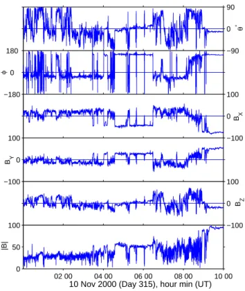
1422 E. A. Lucek et al.: Cluster magnetic field measurements in the magnetosheath −90 0 90 θ ° −180 0 180 φ ° −100 0 100 B X −100 0 100 BY −100 0 100 B Z 02 00 04 00 06 00 08 00 10 00 0 50 100 |B|
10 Nov 2000 (Day 315), hour min (UT)
Fig. 1. Spin averaged magnetic field data in GSE coordinates from Cluster 4 recorded between 00:00 and 10:00 UT on 10 November 2000 (day 315). Panels show magnetic field elevation and longitude angles in degrees, the three components and the magnitude in nT.
the magnetopause surface, EMIC waves are less likely to be found. Mirror structures, however, are found to be very common in this region (Lucek et al., 1999).
Single spacecraft measurements can be used to calculate the scale sizes of mirror structures along the flow direction, if the flow velocity is known, but are not sufficient to de-termine the scale size and orientation in three dimensions. Dual spacecraft observations provide more information, but still leave some ambiguities in establishing the characteris-tics of these features (Fazakerley and Southwood, 1994a,b; Hubert et al., 1998; T´atrallyay and Erd¨os, 2000). In prin-ciple, simultaneous four-point measurements can be used to determine mirror mode size and scale in three dimensions, as well as any dependence of these properties on other parame-ters, such as magnetosheath flow velocity and magnetic field orientation relative to the flow. The separation of the space-craft relative to the scale size of the structures is important, however, with the exception of two satellites separated along the flow direction. If two spacecraft see completely different features, then this implies that the scale size along the space-craft separation vector is smaller than the spacespace-craft separa-tion magnitude, but the exact value cannot be deduced. If a spacecraft pair see identical features, then it is implied that the scale length in that direction is significantly longer than the spacecraft separation, but again the value cannot be cal-culated. Most information is gained when a spacecraft pair sees similar, but not identical signatures. Under these
condi-tions, when the scale along the spacecraft separation vector on which variations in the structures occur is of the order of the separation magnitude, then comparison of the signatures at the two satellites can be used to make an estimate of the gradient of the magnetic field change. Therefore, in order to build up a complete picture, observations made with different tetrahedron sizes and orientations are needed.
In this paper, we identify an interval when the magnetic field signatures are consistent with mirror-mode structures. During this time, the tetrahedron configuration was such that pairs of spacecraft had separation vectors approximately aligned with three key directions: the direction of maximum variance of the magnetic field fluctuations, which is close to the background magnetic field direction and, in this case, predominantly in the ZGSEdirection; the direction of
mini-mum variance, which is close to the estimated magnetopause normal direction; and the intermediate variance direction, which, in this case, is likely to be approximately aligned with the magnetosheath flow vector. We present an analysis of the scale lengths in each of these directions.
2 Correlation of signatures between different space-craft pairs
Figure 1 shows an overview of the magnetosheath data recorded by Cluster 4 on 10 November 2000. The pan-els show the magnetic field elevation angle, the magnetic field longitude angle, and three components, all in GSE co-ordinates, and the magnetic field magnitude. The angles are shown in units of degrees, and the field components and magnitude are in nT. Data at a resolution of one vec-tor per spacecraft spin are shown. Two main intervals of compressional wave activity occur, between ∼ 01:30 and
∼03:30 UT, and between ∼ 06:50 and 08:55 UT. These in-tervals are separated by several magnetopause encounters (Dunlop et al., 2001, this issue). The final crossing in this set, at ∼ 06:20 UT, was caused by a large change in up-stream solar wind conditions, observed by Wind at approxi-mately (83.5 RE, −86.5 RE,7.0 RE) GSE, when the solar
wind velocity increased from 640 to 870 km/s at 06:20 UT with an associated density rise, causing a significant pulse in solar wind ram pressure. We identify the magnetic field signatures during these intervals as consistent with mirror-mode structures. They are strongly compressive and close to linearly polarised, with a maximum variance direction that lies within ∼ 20◦of the background magnetic field direction.
The minimum variance direction lies within 10–25◦of the
lo-cal magnetopause normal, estimated as described by Dunlop et al. (2001, this issue), suggesting that the structures lie in a plane approximately parallel to the magnetopause bound-ary. Therefore, although we are unable to make a defini-tive mode identification, we assume that these signatures are mirror-mode structures.
The typical duration of the mirror structures observed on this day is only 2–3 s, which we ascribe to the high upstream solar wind velocity, and the location of the spacecraft on the
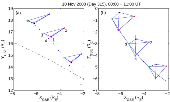
−8 −6 −4 −2 12 13 14 15 16 17 18 19 X GSE (RE) Y GSE (R E ) −8 −6 −4 −2 −7 −6 −5 −4 −3 −2 −1 0 X GSE (RE) Z GSE (R E ) 3 4 1 2 1 2 3 4 10 Nov 2000 (Day 315), 00:00 − 11:00 UT (a) (b)
Fig. 2. Cluster orbit and tetrahedron configuration on 10 November 2000 (day 315) in (a) the X − YGSEplane, and (b) the X − ZGSEplane.
The orbit track of Cluster 3 is shown: dots indicate hours, and the asterisk shows the start of the interval. A dotted line indicates that the component not plotted, e.g. ZGSE in (a), is negative, while a solid line indicates that the third component is positive. The tetrahedron is
shown, expanded by a factor 10, every 4 hours with the Cluster spacecraft represented using the usual colour convention (1-black, 2-red, 3-green, 4-magenta). The dashed line on (a) shows a cut through a Sibeck model magnetopause location for the observed upstream solar wind conditions.
dusk flank, where the magnetosheath plasma has been accel-erated to a significant fraction of the solar wind speed. Since the duration of each mirror drop out is so short, we use the magnetic field data at 22 vectors/second, calibrated as de-scribed by Balogh et al. (2001, this issue), for the analysis presented in the following sections.
Figure 2 shows the configuration of the Cluster satellites between 00:00 and 11:00 UT on 20 November 2000, which covers the period in which mirror structures were observed. Panel (a) shows the spacecraft separation projected onto the
X − YGSEplane and panel (b) plots the orbit projected onto
the Y − ZGSEplane. The dashed line indicates the location of
a Sibeck model magnetopause (Sibeck et al., 1991), with in-put parameters appropriate for the upstream solar wind con-ditions, which is included for reference. The orbit of one spacecraft (Cluster 3) is shown in each plot, with hourly markers plotted as dots on the orbit. The dotted portion of this line indicates when the third component in each case is negative, and the solid portion of the line indicates that the third component is positive. For example, in Fig. 2a, the tetrahedron is below the X − ZGSE plane, i.e. with
nega-tive ZGSE throughout. The asterisk indicates the start of the
interval. The tetrahedron, expanded by a factor 10 relative to the reference orbit, is shown every four hours with black, red, green and magenta representing spacecraft 1, 2, 3 and 4, respectively.
In this paper, we first present the analysis of mirror structures seen during one minute (08:23–08:24 UT) on 10 November 2000. These mirror structures are representative
of an hour of mirror activity which was bounded by magne-topause encounters. We then consider a second interval con-taining mirror structures, from the previous minute of data acquisition which, while less typical, demonstrates a further property of these mirror-mode observations.
2.1 Interval 1: 08:23–08:24 UT
Figure 3 shows a short interval of mirror activity observed between 08:23 and 08:24 UT on 10 November 2000. The format of the panels is the same as in Fig. 1, but here the data from all four spacecraft are plotted, with black, red, green and magenta used to represent data from spacecraft 1, 2, 3 and 4, respectively. Although there are obvious differences between some spacecraft pairs, the power spectra of the mag-netic field magnitudes are statistically similar within errors. Figure 4 shows the power spectra of the magnetic field com-ponents in the maximum variance directions, calculated us-ing a multi-taper method (Percival and Walden, 1993), ob-served by the 4 spacecraft during two minutes of mirror ac-tivity. The same colour convention is used. The blue trace shows the power spectrum of the intermediate variance com-ponent from Cluster 3 in order to demonstrate that the power is predominantly in compressional, with linearly polarised fluctuations. The power spectra of the intermediate variance components at the other spacecraft are similar. Two minutes of data are used in order to resolve better the low end of the frequency spectrum. The traces from the four spacecraft are similar within statistical errors, indicated by the 90%
confi-1424 E. A. Lucek et al.: Cluster magnetic field measurements in the magnetosheath −90 0 90 θ ° −180 0 180 φ ° −20 0 20 Bx −50 0 50 By 0 50 100 Bz 08 23 000 08 23 15 08 23 30 08 23 45 08 24 00 50 100 |B|
10 Nov 2000 (Day 315), hour min sec (UT)
Fig. 3. One minute of magnetic field data showing mirror-like ac-tivity. Panels have the same format as in Fig. 1. Data from all four spacecraft are shown using the same colour-coding as in Fig. 2.
dence level shown on the bottom left of the plot. Each power spectrum of the maximum variance component has the same form, with approximately equal power as a function of fre-quency at the lowest frequencies (although the trace for Clus-ter 4 has a suggestion of a broad enhancement at ∼ 0.15 Hz) with a break in the spectrum between 0.3–0.4 Hz, after which the power falls off as frequency increases. There is signifi-cantly lower power in the intermediate variance component at Cluster 3, and at each of the other spacecraft (not shown). The position of the break point corresponds to the scale of the shortest mirror structure, of ∼ 2–3 s, and is at a signifi-cantly lower frequency than the local proton gyro-frequency, shown on Fig. 4 as a vertical dashed line. From Fig. 4 it can be seen that the break in the power spectrum occurs at the same place for each of the traces, and that the power levels are the same within the 90% confidence limit. Therefore al-though the particular structures may be different, the sets of mirror structures observed by the four satellites are statisti-cally similar.
From the orbital configuration at 08:00 UT (the last ex-panded tetrahedron shown on the orbit segment in Fig. 2), it can be seen that the position vectors of Cluster 1 (black) and 4 (magenta) relative to Cluster 3 (green) lie approxi-mately parallel to the nominal magnetopause in the X −YGSE
plane, but that Cluster 1 is at a similar Z location, while Clus-ter 4 is at a significantly lower position in Z. ClusClus-ter 2 (red) lies significantly further from the magnetopause, deeper in the magnetosheath, at a distance of ∼ 660–700 km along the
10−2 10−1 100 101 102 10−6 10−4 10−2 100 102 Power (n T 2 /Hz) 10 Nov 2000 08:22 - 08:24 UT f (Hz)
Fig. 4. Power spectra of the maximum variance magnetic field com-ponent measured by all four spacecraft between 08:22 and 08:24 UT of 10 November 2000 (day 315). The blue line shows the power spectrum of the intermediate variance component observed by Clus-ter 3. The vertical dashed line shows the proton gyro-frequency es-timated using the background magnetic field magnitude of ∼ 65 nT.
magnetopause normal from satellites 1 and 3. The magnetic field at this time is only 11 − 13◦from the ZGSEdirection,
and so Cluster 1 and Cluster 4 are likely to lie close to the same field line since they are very close in the X − YGSE
plane with a large separation in ZGSE(Fig. 2b).
Figure 5 shows a comparison of the magnetic field magni-tudes observed at the different spacecraft. Cluster 3 is used as the reference spacecraft for three of the panels, but a com-parison of Cluster 1 and 4 is also shown because their relative position vector is likely to be nearly parallel to the average magnetic field direction. The top panel shows the magnetic field magnitude observed at spacecraft 3 (in green) and at spacecraft 1 (in black). From this panel, it is clear that there is an extremely good correlation between the two satellites throughout the interval, and both satellites sample essentially the same structures. This is also clear from the top panel of Fig. 6, which shows the same data when the trace from Clus-ter 1 has been shifted by 0.61 s. Figure 7 shows the cross-correlation function between these two data sets in the black trace. The cross-correlation coefficient has a peak value of 0.98, and a time lag of 0.61 s using 1346 data points.
From the orbit plots it can be seen that the separation vec-tor between Cluster 1 and Cluster 3 lies approximately paral-lel to the magnetopause boundary in the X − YGSE plane,
while there is little separation in Z. Although we do not have measurements of the magnetosheath flow velocity vec-tor on this day, it is likely that it lies close to the Cluster 1 – Cluster 3 spacecraft separation vector. Variance analysis of the mirror structures shows that the Cluster 1 – Cluster 3 separation vector also lies within ∼ 15◦of the intermediate variance direction. During this interval, the spacecraft sep-aration along the X − YGSE plane was ∼ 490 km, and so
0 40 80 |B| (nT) 0 40 80 |B| (nT) 1−3 0 40 80 |B| (nT) 4−3 08 23 000 08 23 15 08 23 30 08 23 45 08 24 00 40 80
10 Nov 2000 (Day 315), hour min sec (UT)
|B| (nT)
2−3
4−1
Fig. 5. A comparison of the magnetic field magnitude seen at dif-ferent spacecraft pairs. The panels show Cluster 1 (black) and 3 (green), Cluster 4 (magenta) and 3 (green), Cluster 2 (red) and 3 (green) and finally Cluster 1 (black) and 4 (magenta).
this location in the magnetosheath, so far in the dusk flank, we expect the magnetosheath velocity to have been acceler-ated back to a significant fraction of the solar wind ity in this region. The estimate of the magnetosheath veloc-ity is consistent, therefore, with the solar wind velocveloc-ity of 870 km/s observed by Wind, lying upstream. Using the esti-mated magnetosheath velocity implies that the scale size of the mirror structures in the flow direction, which is likely to be close to the intermediate variance direction, is of the or-der of 1500–3000 km, which is significantly larger than the spacecraft separation. This estimate assumes that the veloc-ity is entirely along the Cluster 1 – Cluster 3 separation vec-tor, but the excellent correlation between the signatures at the two spacecraft suggests that the two velocity components perpendicular to the separation vector are likely to be small relative to the velocity magnitude.
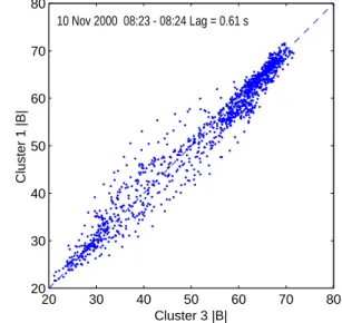
Figure 8 shows the scatter plot of the two data sets, with the lag of 0.61 s applied. There is clearly a very high corre-lation, but although the extrema show little scatter, the in-termediate magnetic field values show more scatter. This arises from very small changes in the delay between the two satellites, which has the largest effect when the gradient of the field is large. If higher frequency waves were superim-posed on the mirror structures, then the relative movement between such waves and the mirror structures would cause greater scatter at the extrema.
The second panel of Fig. 5 shows the magnetic field mag-nitude seen by Cluster 3 (in green) and that measured by Cluster 4 (in magenta). Comparison with the top panel shows that the correlation is significantly lower, with the satellites apparently sampling different structures in some regions as a result of their different locations, while observing simi-lar structures in others. The cross-correlation function
be-0 40 80 |B| (nT) 0 40 80 |B| (nT) 1−3 0 40 80 |B| (nT) 4−3 08 23 00 08 23 15 08 23 30 08 23 45 08 24 00 0 40 80 |B| (nT)
10 Nov 2000 (Day 315), hour min sec (UT)
2−3
4−1
Fig. 6. The same data as in Fig. 5, but one data set is shifted by the time of the peak cross-correlation coefficient. Cluster 3 is used as the reference in the top three panels, and Cluster 1 is used as the reference in the bottom panel.
tween these two traces is shown in Fig. 7 by the solid ma-genta line. Here, the peak correlation coefficient is lower (0.54) at a longer lag of 1.8 s, calculated using 1346 data points. The plots of the Cluster tetrahedron orbit in Fig. 2 show that this spacecraft pair has a very similar separation vector in the X − YGSE plane as Cluster 1 and 3, but that
they have a significantly larger separation in Z. Comparison of the spacecraft separation vector with the maximum vari-ance direction of the mirror structures shows that the mir-ror structures lie at ∼ 40◦to the vector separating Cluster 3
and Cluster 4. Assuming that the same structures are ob-served by Cluster 3 and Cluster 4, and that the structures are elongated along the maximum variance direction, Cluster 4 passes through each mirror structure at a location separated by approximately 500 km along the maximum variance di-rection from the Cluster 3 crossing location. Although the magnetosheath velocity vector is not known, assuming that the plasma velocity is close to the convection velocity mea-sured between Cluster 1 and Cluster 3, an expected time de-lay occurs between the signatures at Cluster 4 and Cluster 3 which is ∼ 0.6 s, significantly shorter than the observed de-lay. A more precise comparison is not possible without direct measurement of the magnetosheath velocity vector.
The second panel of Fig. 6 shows the two data sets where the magnetic field measured by Cluster 4 has been shifted by 1.8 s. From this plot, it can be seen that when the two satel-lites appear to observe the same structures, the time delay is not as stable in this case as for the previous case. The bot-tom panel of Fig. 6 shows that a similar situation is observed when data from Cluster 1 and Cluster 4 are compared. These spacecraft lie almost vertically one above the other, but still show a significant time delay at the peak correlation (shown in the dotted magenta line in Fig. 7). Since Cluster 1 and
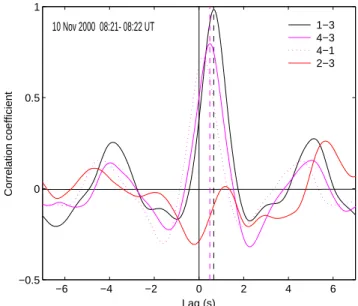
1426 E. A. Lucek et al.: Cluster magnetic field measurements in the magnetosheath −6 −4 −2 0 2 4 6 −0.5 0 0.5 1 Lag (s) Correlation coefficient 1−3 4−3 4−1 2−3 10 Nov 2000 08:23 - 08:24 UT
Fig. 7. Cross-correlation functions between the spacecraft pairs shown in Fig. 5: Cluster 1 and 3 (solid black trace), Cluster 4 and 3 (solid magenta trace), Cluster 4 and 1 (dotted magenta trace) and finally Cluster 2 and 3 (solid red trace).
Cluster 3 observe the same structures with little or no evolu-tion during the time taken for the structures to convect from one to the other, the difference in the signatures observed by Cluster 1 and 4 (and Cluster 3 and 4) is likely to indi-cate a spatial variation rather than a temporal one. The lower level of correlation and the variable time delay might reflect changes in the size and form of the mirror structures along the maximum variance direction. There might also be a con-tribution to the lower correlation level from the two craft occasionally observing different structures. If a space-craft separation vector were to lie parallel to the maximum variance direction, then a good correlation at near zero lag should be observed. One such example has been found which will be discussed in the next section.
The third panel in Fig. 5 shows the magnetic field magni-tudes measured by Cluster 2 (red) and 3 (green). Here, there is a low correlation between the two signals, and the red trace in Fig. 7 shows that the peak correlation coefficient is less than 0.25. Any impression of anti-correlation between the traces is likely to arise from the statistically similar nature of the data, and is not evident in the cross-correlation function. There are occasions when the data from the two spacecraft are similar, but it is not clear whether these similarities occur by chance, or whether they represent real, but rare occasions when the same feature is seen at both spacecraft. The orbit plot shows that the two spacecraft have approximately the same Z coordinate, but that they have a separation of about 660 km projected along the magnetopause normal (derived from Dunlop et al. (2001, this issue)) and that Cluster 2 is situated deeper in the magnetosheath than Cluster 3 or the other spacecraft. It appears, therefore, that the largest varia-tion in mirror structure characteristics occurs along the mag-netopause normal, and that the scale length in this direction is
20 30 40 50 60 70 80 20 30 40 50 60 70 80 Cluster 3 |B| Cluster 1 |B| 10 Nov 2000 08:23 - 08:24 Lag = 0.61 s
Fig. 8. A scatter plot of the magnetic field magnitude measured at Cluster 1 plotted against that measured at Cluster 3, at a time delay of 0.61 s, which corresponds to the peak of the cross-correlation function.
generally smaller than the spacecraft separation of ∼ 660 km. 2.2 Interval 2: 08:22–08:23 UT
Figure 9 shows the data recorded between 08:22 and 08:23 UT, a minute earlier than the data discussed in the pre-vious section. The format of Fig. 9 is the same as Figs. 5 and 6, and Fig. 10 shows the equivalent set of correlation func-tions as shown in Fig. 7. In this case, the maximum variance direction of the mirror structures is within only ∼ 5◦of the
mean field direction, and is also closer to the ZGSEdirection.
Again, there is an excellent correlation between Cluster 1 and Cluster 3, with a delay of 0.66 s, which is consistent with a velocity of about 815 km/s. In this case, however, Cluster 4 and Cluster 3 show very well correlated signatures, with a de-lay of 0.48 seconds which is consistent with the same veloc-ity, assuming that the structures are closely aligned with the maximum variance direction, which, in this case, lies within 27◦of the Cluster 3 – Cluster 4 separation vector.
Cluster 1 and Cluster 4, which lie almost vertically above one another at the same X − Y location, now show a well correlated signature with a shorter delay, also consistent with the structure being aligned with the maximum variance di-rection, which is within 3◦of the mean magnetic field
direc-tion and 18◦ of the spacecraft separation vector. Although
satellites 1 and 4 see the same structures, variations are seen between the depths of the mirror structures at Cluster 1 and 4, which have a separation along the maximum variance di-rection of about 750 km. This variation is not seen when comparing Cluster 1 and Cluster 3, which have a separation vector which is nearly at 90◦to the maximum variance direc-tion. Once again, Cluster 2 and Cluster 3, which have a sep-aration along the magnetopause normal of ∼ 660 km, do not observed the same structures, and in this case, the maximum
0 40 80 |B| (nT) 0 40 80 |B| (nT) 1−3 0 40 80 |B| (nT) 4−3 08 22 00 08 22 15 08 22 30 08 22 45 08 23 00 0 40 80 |B| (nT)
10 Nov 2000 (Day 315), hour min sec (UT)
2−3
4−1
Fig. 9. A comparison of the magnetic field magnitudes measured at different spacecraft pairs in the same format as Figs. 5 and 6.
correlation coefficient is even lower than in the previous ex-ample.
3 Discussion
We have demonstrated the potential of simultaneous four-point measurements using very simple analysis methods ap-plied to 2 short intervals of mirror activity. The results sug-gest that within these mirror structures, the correlation length along the flow direction is of the order of 1500–3000 km. The scale of the mirror structures is smallest along the estimated magnetopause normal in both examples, which is within 10– 25◦of the minimum variance direction, and is approximately
perpendicular to both the mirror structure maximum variance direction (close to the background magnetic field vector) and the flow direction. No correlation is observed between space-craft separated by approximately 660 km along this direction. In the direction along the maximum variance direction, variations between spacecraft are observed on scales of
∼750 km. The delay between observations at different spacecraft pairs during interval 2 (08:22–08:23 UT) appears to be consistent with that expected for structures elongated along the maximum variance direction, but significant dis-crepancies appear to exist in the delays found in interval 1 (08:23–08:24 UT). It is not clear what causes this effect, al-though it might arise from the mirror structures having dif-ferent orientations between the two intervals. One observed difference between the two intervals is that during interval 2, Cluster 1, 3, and 4 have much smaller separations along the minimum variance direction than during interval 1. The level of correlation, therefore, might arise from a periodicity in the mirror structure field (e.g. Fazakerley and Southwood, 1994a,b; T´atrallyay and Erd¨os, 2000), where the spacecraft sample different, but statistically related structures. We note,
−6 −4 −2 0 2 4 6 −0.5 0 0.5 1 10 Nov 2000 08:21- 08:22 UT Lag (s) Correlation coefficient 1−3 4−3 4−1 2−3
Fig. 10. The cross-correlation functions for the data shown in Fig. 9, in the same format as Fig. 7.
however, that direct measurements of the magnetosheath flow velocity are necessary in order to explore this further. Our results are in agreement with previous observations (e.g. Fazakerley and Southwood, 1994b; Hubert et al., 1998) which showed that the mirror structures were elongated ap-proximately along the background magnetic field direction. Fazakerley and Southwood (1994b) showed that the scale transverse to the structure was of the order of 1000–3000 km, which is consistent with our measurement of the scale along the flow direction, but they note that this estimate might have contributions from two different scales perpendicular to the maximum variance direction, depending on how the space-craft sampled the structures. Hubert et al. (1998) showed that the shortest scale was approximately along the magnetopause normal, consistent with our results, but their estimate of this scale length was ∼ 1300–1900 km, which is significantly longer than our upper limit of ∼ 660 km. Hubert et al. (1998) found that the longest scale length, approximately along the background field direction, exceeded ∼ 3000 km. This is not inconsistent with our observations of changes in the signa-tures between spacecraft separated by ∼ 750 km along the maximum variance direction (∼ parallel to the background magnetic field direction), since this implies that the extent of the structures in this direction is significantly larger than the spacecraft separation. Hubert et al. (1998) found an interme-diate scale exceeding ∼ 2500 km which is larger than our ob-servation of a scale of ∼ 1500–3000 km approximately along the flow direction which, is in this case, is nearly perpendic-ular to both the background magnetic field and the estimated magnetopause normal.
From just two intervals, the tetrahedral configuration does not change sufficiently to make a full study of the mirror structure size and orientation. Examination of further
ex-1428 E. A. Lucek et al.: Cluster magnetic field measurements in the magnetosheath amples where the magnetic field has a different orientation
is essential to confirm which directions provide the best or-der for the observations. A statistical study of many intervals with different spacecraft separations and configurations rela-tive to the flow and magnetic field directions can, in principle, be used to calculate the correlation lengths of the structures along each direction. A further consideration is the possible dependence of the mirror structure scale size on the magne-tosheath flow velocity, which should be taken into account in such a study. If mirror structure scale sizes in at least two directions are of the order of the spacecraft separation, then methods such as normal fitting and time delay analysis for velocity calculations (e.g. Schwartz, 1998) must be applied with caution, since the structures might show significant cur-vature on the spacecraft separation scales.
Acknowledgements. Analysis of Cluster data at Imperial College is
supported by PPARC. Details of the upstream solar wind conditions were obtained from Wind plasma data made available by K. Ogilvie at NASA GSFC through the CDAWeb, set up by the NASA/GSFC Space Physics Data Facility and the National Space Science Data Center. The location of Wind was found using the NASA/GSFC SSCWeb.
Topical Editor G. Chanteur thanks C. Mazelle and another ref-eree for their help in evaluating this paper.
References
Anderson, B. J., Fuselier, S. A., Gary, S. P., and Denton, R. E.: Magnetic spectral signatures in the Earth’s magnetosheath and plasma depletion layer, J. Geophys. Res., 99, 5877–5891, 1994. Balogh, A., Carr, C. M., Acu˜na, M. H., Dunlop, M. W., Beek, T.
J., Brown, P., Fornacon, H., Georgescu, E., Glassmeier, K.-H., Harris, J., Musmann, G., Oddy, T., and Schwingenschuh, K.: The Cluster Magnetic Field Investigation: overview of in-flight performance and initial results, Ann. Geophysicae, (this issue) 2001 .
Dunlop, M. W., Balogh, A., Cargill, P., and the FGM team: Clus-ter observes the Earth’s magnetopause: co-ordinated four-point measurements, Ann. Geophysicae, (this issue), 2001 .
Erd¨os, G. and Balogh, A.: Statistical properties of mirror mode structures observed by Ulysses in the magnetosheath of Jupiter,
J. Geophys. Res., 101, 1–12, 1996.
Fazakerley, A. N. and Southwood, D. J.: Mirror instability in the magnetosheath, Adv. Space Res., 14, 7, 65–68, 1994a.
Fazakerley, A. N. and Southwood, D. J.: Theory and observations of magnetosheath waves, in Solar wind sources of magnetospheric ultra-low frequency waves, Geophys. Monogr. Ser., 81, (Eds) En-gebretson, M., Takahashi, K., and Scholer, M., 147–158, AGU Washington, D. C., 1994b.
Hubert, D., Lacombe, C., Harvey, C. C., Moncuquet, M., Russell, C. T., and Thomsen, M. F.: Nature, properties, and origin of low-frequency waves from an oblique shock to the inner mag-netosheath, J. Geophys. Res., 103, 26 673–26 798, 1998. Lacombe, C., Belmost, G., Hubert, D., Harvey, C. C., Mangeney,
A., Russell, C. T., Gosling, J. T., and Fuselier, S. A.: Density and magnetic field fluctuations observed by ISEE 1–2 in the quiet magnetosheath, Ann. Geophysicae, 13, 343–357, 1995. Lucek, E. A., Dunlop, M. W., Balogh, A., Cargill, P., Baumjohann,
W., Georgescu, E., Haerendel, G., and Fornacon, K.-H.: Identi-fication of magnetosheath mirror modes in Equator-S magnetic field data, Ann. Geophysicae, 17, 1560–1573, 1999.
Percival, D. B. and Walden, A. T., Spectral analysis for physical ap-plications, Cambridge University Press, Cambridge, UK, 1993. Phan, T.-D., Paschmann, G., Baumjohann, W., Sckopke, N., and
L¨uhr, H.: The magnetosheath region adjacent to the dayside mag-netopause: AMPTE/IRM observations, J. Geophys. Res., 99, 121–141, 1994.
Price, C. P., Swift, D. W., and Lee, L.-C.: Numerical simulation of nonoscillatory mirror waves at the Earth’s magnetosheath, J. Geophys. Res., 91, 101–112, 1986.
Schwartz, S. J.: Shock and discontinuity normals, Mach num-ber, and related parameters, in: Analysis methods for multi-spacecraft data, (Eds) Paschmann, G. and Daly, P. W., ESA Pub-lications Division, Noordwijk, The Netherlands, 1998.
Sibeck, D. G., Lopez, R. E., and Roelof, E. C.: Solar wind control of the magnetopause shape, location and motion, J. Geophys. Res., 96, 5489–5495, 1991.
T´atrallyay, M. and Erd¨os, G.: Mirror mode fluctuations in the terres-trial magnetosheath, in: The Solar Wind-Magnetosphere System 3, (Eds) Biernat, H. K., Farrugia, C. J., and Vogl, D. F., Verlag der ¨Osterreichischen Akademie der Wissenschaften, 2000. Tsurutani, B. T., Smith, E. J., Anderson, R. R., Ogilvie, K. W.,
Scudder, J. D., Baker, D. N., and Bame, S. J.: Lion roars and non-oscillatory drift mirror waves in the magnetosheath, J. Geophys. Res., 87, 6060–6072, 1982.