Economic theory and estimation of the demand for consumer durable goods and their utilization : appliance choice and the demand for electricity

-N

ECONOMIC THEORY AND ESTIMATION OF THE DEMAND FOR CONSUMER DURABLE GOODS AND THEIR UTILIZATION:

APPLIANCE CHOICE AND THE DEMAND FOR ELECTRICITY

by

Jeffrey Alan Dubin

A.B. University of California, Berkeley (1978)

Submitted In Partial

to the Department of Economics Fulfillment of the Requirements

For the Degree of Doctor of Philosophy

at the

Massachusetts Institute of Technology May 1982

Signature of Author

Signature Red acted

Certified by Accepted by_

Signature

Signature

Redacted

Redacted

Archives JUN 2 2 1982

1

I'POP011IF's

DURABLE GOODS AND THEIR UTILIZATION:

APPLIANCE CHOICE AND THE DEMAND FOR ELECTRICITY by

Jeffrey Alan Dubin

~

Submitted to the Department of Economics on May 17, 1982 in partial fulfillment of the requirements for the Degree of Doctor of Philosophy at the Massachusetts Institute of Technology

ABSTRACT

This thesis develops the theory of durable choice and utilization. The basic assumption is that the demand for energy is a derived demand arising through the production of household services. Durable choice is associated with the choice of a particular technology for providing the household service. Econometric systems are derived which capture both the discrete choice nature of appliance selection and the determination of continuous conditional demand.

Conditional moments in the generalized extreme value family are derived to extend discrete continuous econometric systems in which discrete choice is assumed logistic. An efficiency comparison of various two-stage consistent estimation techniques applied to a single equation of a dummy endogenous simultaneous equation system is undertaken and asymptotic distributions are derived for each estimation method.

Using the National Interim Energy Consumption Survey (NIECS) from 1978

we estimate a nested logit model of room air-conditioning, central air-conditioning, space-heating, and water heating. The estimated probability choice model is used to forecast the impacts of proposed building standards for newly constructed single family detached residences. Monthly billing data matched to NIECS is analyzed permitting seasonal estimation of the demand for electricity and natural gas ty households.

The theory of price specification for demand subject to a declining rate struc-ture is reviewed and tested. Finally, consistent estimation procedures are used in the presence of possible correlation between dummy variables indicating appli-ance ownership and the equation error. The hypothesis of simultaneity in the demand system is tested.

Signature redacted

Thesis Supervisor: Dr. Daniel L. McFadden Title: Professor of Economics

-3-S JEFFREY ALAN DUBIN

BIOGRAPHY Personal Data

Date of Birth: _{January 24, 1957 (Berkeley, California)} Married to Jacqueline Mary Dubin

Education

A.B. _{(Economics) University of California, Berkeley, 1978, with} highest honors and with great distinction.

Academic Appointments

Reader (Economics), University of California Berkeley, 1977.

Research Assistant (Economics), Massachusetts Institute of Technology, with Professor Daniel L. McFadden, 1979-1981.

Teaching Assistant (Economics), Massachusetts Institute of Technology, Graduate Applied Econometrics (appointment for Spring 1982).

Memberships in Scholarly and Professional Organizations Phi Beta Kappa

American Economic Association The Econometric Society

University of California, Lifetime Alumnus Professional Service

Referee to Review of Economic Studies and Bell Journal of Economics Fellowships, Scholarships, Honors, and Awards

Edward Frank Kraft Prize 1974-1975

Honor Roll 1974-1978 University of California, Berkeley Phi Beta Kappa 1978

Department Citation in Economics, University of California, Berkeley, 1978

ACKNOWLEDGEMENTS

There are several people who have made this thesis possible.

First I wish to thank my thesis committee Daniel McFadden, Ernst Berndt, and Franklin Fisher. Ernie and Frank read and commented on early drafts of this work and provided general guidance during this last year. My mentor and friend Dan McFadden provided very important advice and support and much of his valuable time. It has been a great pleasure to work as an apprentice under Dan during the last three years and I owe him a principal intellectual debt in teaching me the art and science of econometrics.

I wish to acknowledge further the support and understanding of my parents over the many years of my education. This thesis must be dedicated to them. I want to mention my oldest and dearest friend, Harry Kraus, who often encouraged me to complete this work and who introduced me to my wife Jackie. Jackie suffered with me the joys and trials of completing an empirical thesis. I am indebted to her for her help with typing and assembling of the manuscript.

I acknowledge the support of NSF 7920052-SOC., NSF 80-16043-DAR through Dan McFadden, the typing staff of the MIT Energy Laboratory, and the Department of Economics at MIT for fellowship support during the first two years in graduate school.

Jeffrey Alan Dubin May 17, 1982

-5-TABLE OF CONTENTS

Pages Introduction and Summary

1. Overview ... 2. The Residential Energy Consumption Process... 3. _{Economic and Statistical Issues in Modelling}

the Choice of Durables and their Utilization.... 4. Organization of Thesis... Chapter One - On the Theory and Estimation of Consumer

Durable Choice and Utilization

1. Introduction... 2. Classical Models of Consumer Durable Choice... 3. Consumer Durable Choice and Appliance Technology 4. Appliance Technology and Two-Stage Budgeting....

5. Econometric Specification for Models of Durable Utilization... 6. Summary and Conclusions... Chapter Two - Rate Structure and Price Specification in

the Demand for Electricity 1. 2. 3. 4. 5. Introduction...

Specification of Price: Theory...

Specification of Price: Empirical Results..

Measurement of Price: Theory and Estimation

Summary and Conclusions...

Chapter Three - Estimation of Nested Logit Model for Appliance Holdings

1. Introduction... 2. Nested Logit Model of Appliance Choice... 3. Residential Heating and Comfort... 4. Room Air Conditioner Choice Model... 5. Water Heat Choice Model... 6. Space Heat Choice System...

7. Central Air Conditioning Choice ...

8. The Effect of the ASHRAE 90-75 Building Standards on the Saturation of Alternative HVAC Systems.... 9. Summary and Conclusions...

... 7 ... 9 ... ... 11 ... 13 17 22 29 44 52 59 61 62 71 85 106 ... 108 ... 109 ... 116 ... 119 ... .... 126 ... 133 ... 149 ... 156 ... 158 Chapter Four 1. Introduction ... 2. Demand for Electricity by Aggregated Billing Period 3. Demand for Natural Gas by Aggregated Billing Period 4. Consistent Estimation of the Demand for Electricity and Natural Gas ... 5. Summary and Conclusions... ... 159

... 160

... 171

... 173

Appendix One - A Review of the Appended NIECS Data Base and

the Monthly Billing Data... 1. The Appended NIECS Data Base... 2. Reprocessing the Monthly Billing Data...

3. Use of Billing Data to Obtain Marginal Prices... 4. Adaptation of Annual Thermal Model to Monthly

Billing Data...

5. Case Study of Household Number 1271... 6. Computer Programs and Selected Output... Appendix Two - Conditional Moments in the Generalized

Extreme Value Family... Appendix Three - Two-Stage Single Equation Estimation

Methods: An Efficiency Comparison... Glossary... References---... 189 191 194 202 206 223 236 259 ... 296 ... 322 ... 325

-7-INTRODUCTION AND SUMMARY

Economic Theory and Estimation of the Demand for Consumer Durable Goods and their Utilization: Appliance Choice and the Demand for Electricity

I. Overview

In the years 1947 to 1972 the United States experienced an almost seven-fold increase in the use of electricity. The early 1970's brought the interwined problems of depleting oil resources, increased

dependence on oil imports and a heightened need for a consensus in national energy policy. However, increasing concern over the safety of nuclear power mitigated the trend toward pervasive electrification and the nation's all-electric future.

The need to quantify the responsiveness of electricity utilization to various energy policies rose rapidly in the energy turbulent 1970's. This need was felt all the way down to home owners who became concerned with efficiency and costs of alternative heating and cooling systems. Of

course home owners who had witnessed an increase in their energy budget from 26% in 1972 to 33% in 1980 knew all too well that the composition of their appliance stock greatly influenced their usage.1

Energy researchers also noted the importance of durable stocks in the energy demand process.2 Yet, only in very recent attempts have econometric simulation models allowed policy scenarios simultaneously to affect appliance holdings and resultant usage. In one direction are aggregate studies which fit average appliance saturations to the time

trend of income, prices, and other socio-economic variables. This approach is best exemplified in the modeling efforts of Hirst and Carney (1978). Other aggregate based studies are extensively reviewed in Hartman (1978, 1979).3

In contrast to the aggregate studies, several attempts to model jointly the demand for appliances and the demand for fuels by appliance

have been completed using cross-sectional micro level survey data.4

The use of disaggregated data is desirable as it avoids the confounding effects of either misspecification due to aggregation bias or

misspeci-fication due to approximations in rate data.

Either approach has a common objective in modeling household energy consumption patterns from which to evaluate conservation and load management policies. For example, can we evaluate the welfare and distributional impacts of proposed government policies to decontrol the price of natural gas? How rapidly do consumers repond to rising energy prices? What are the differences between the energy consumption of owner-occupiers and tenants? What are the implications for public information programs that provide energy efficiency labeling and building and appliance standards? Does the marketplace offer sufficient incentives to pursue appropriate levels of conservation; what actions should govern-ment take, if any, to encourage conservation? Can we quantify the long and short-run responses to policy actions and describe the time path of conservation?

To answer these questions in a logical fashion requires us to conceptualize the residential energy consumption process.

-9-II. The Residential Energy Consumption Process

Figure 1 illustrates the residential energy consumption process. Household demographics, household income, fuel prices, equipment prices, and climate are inputs to a residential choice process which

determines appliance and dwelling characteristics. Included in

appliance characteristics are fuel types, capacities, efficiencies,

and holdings. Included in dwelling characteristics are structure

type, size, and thermal integrity. Given the appliance and housing stock, households react to policy and market variables such as energy prices, efficiency standards, etc. to determine energy usage by

appliance and by fuel type. Each policy question may be traced in its

effects through the diagram in Figure 1. For example, consider a

proposed change in the building code which would require all new

dwellings to meet a baseline thermal integrity standard through wall and ceiling insulation. The increased thermal integrity in the housing stock

would alter the structure of operating and capital costs of available heating and cooling systems available for purchase. Changes in expected operating and capital costs would produce a predictable shift in the saturations of alternative heating and cooling systems. Furthermore, the demand for fuels by appliance would be different to reflect the

increased thermal integrity of the dwelling and the resultant changes

in the marginal costs of providing these services. For details

con-cerning the implementation of a large scale energy forecasting model the reader should consult Goett (1979) and Cambridge Systematics/WEST (1979).

For the purposes of forecasting, the residential energy consumption

Figure 1

The Residential Energy Consumption Process

DDGRAPHIC

jEDULE:

Ha

PLICY

VARIABLES:

ENERGY

FOICASTS

Source: Cambridge Systematics (1979)

USING

AND APLIANCE

CHOICE

HOUSING STOCK

APPLIANCE STOCK

ENERGY

USE

NO

ELECTRICITY

LOAD:

ANNUAL

SEASONAL AND )AILY LOADS

a

decision is made. Conditional on the housing decision, appliance port-folios are chosen by the household, and finally, energy demand is

determined conditional on the choice of appliance stock. For the purposes of estimation, however, it must be recognized that the demand for durables and their use are related decisions by the consumer. Econometric specifications which ignore this fact lead to biased and inconsistent estimates of price and income elasticities. It is to these issues that we now turn.

III. Economic and Statistical Issues in Modelling the Choice of Durables and Their Utilization

Economic analysis of the demand for consumer durables suggests that such demand arises from the flow of services provided by durables ownership. The utility associated with a consumer durable is then best characterized as indirect. Durables may vary in capacity, effi-ciency, versatility, and of course will vary correspondingly in price. Although durables differ, the consumer will ultimately utilize the

durable at an intensity level that provides the "necessary" service. Corresponding to this usage will be the cost of the derived demand for the fuel that the durable consumes. The optimization problem posed is thus quite complex. In the spirit of the theory the consumer unit must weigh the alternatives of each appliance against expectations of future use, future energy prices, and current financing decisions.

The specification of econometric demand systems for fuel

usage presupposes that consumers can detect prevailing marginal fuel rates in the presence of automatic appliances, billing cycle variations, and limited information on appliance operating characteristics.

tests to determine the exogeneity of appliance dummy variables typically included in demand for electricity equations. Their approach derives an indirect utility function which is consistent with the specification of a partial demand equation. The indirect

utility function is used to predict portfolio choice while the

demand equation predicts conditional electricity usage.5 The demand system consists of simultaneous equations with dummy endogenous variables (Heckman (1978, 1979)) and may be thought of as a switch-ing regression with a structure analyzed by Lee (1981), Goldfeld and Quandt (1972, 1973, and 1976), Maddala and Nelson (1974 and 1975), and

Fair and Jaffee (1972).

Employing a logistic discrete choice model of all electric versus all natural gas space and water heat systems combined with conditional demand for electricity, Dubin and McFadden (1979) reject the hypothe-sis that unobserved factors influencing portfolio choice are independent of the unobserved factors influencing intensity of use.

The purpose of this thesis is to analyze the residential demand for electricity and natural gas conditional on the choice of space heat, water heat, central and room air conditioning choice utilizing the

National Interim Energy Consumption Survey (NIECS) 1978 survey of 4081 households. The model developed in this thesis is intended to have the flexibility to be included into a large micro-simulation forecasting system (such as the Residential End-Use Energy Policy

-13-System (REEPS)).6 The thesis further extends the theoretical develop-ment of durable choice and utilization and seeks to examine the

hypothesis of simultaneity between appliance choice and electricity and natural gas demand. The thesis is organized into four chapters and three appendices.

IV. Organization of Thesis

In Chapter One we develop the theory of durable choice and utili-zation. The basic assumption is that the demand for energy is a derived demand arising through the production of household services. The technology which provides the household service is the appliance durable. _{Durable choice is then associated with the choice of a}

particular technology from a set of alternative technologies. Using results from household production theory, we derive econometric systems

which capture both the discrete choice nature of appliance

selection and the determination of continuous conditional demand. Chapter two reviews the theory of price specification and con-siders the comparative static analysis of demand subject to a declining block rate schedule. We further investigate the statistical endogeneity of prices whose construction requires utilization of the observed

consumption level, and determine price specification within a sample of 744 households surveyed in 1975 by the Washington Center for Metropolitan

Studies (WCMS). We finally consider the construction of marginal prices using the WCMS data and monthly billing data from NIECS.

Chapter Three describes the estimation of a discrete choice model for room air-conditioning, central air-conditioning, space heating,

and water heating. The form of the appliance choice model results from the assumption that the unobserved components of utility have a generalized extreme value distribution. A particular form of this distribution is considered which implies that the choice of room air conditioning given the choice of central air conditioing is independent of the choice of space heat system given the choice of central air conditioning. Water heat fuel choice is assumed to depend only on the choice of space heat system.

Chapter Four presents the estimation of the demand for electri-city and natural gas. Consistent estimation procedures are used in the presence of possible correlation between the dummy variables

indicating appliance holdings and the equation error term. We perform tests for simultaneity using the methods of Hausman (1978). Estima-tion is based on monthly billing data matched to each household in the NIECS survey. The monthly billing data provides an excellent time profile of usage which permits the determination of individual seasonal effects.

The main text of the thesis is followed by three technical appendi-ces. The first appendix describes the processing of the NIECS

data and the creation of an appended NIECS data base. It further describes the creation of marginal electricity and natural gas prices based upon the theory of Chapter Two and describes the use of a network thermal model to provide unit energy consumptions for alternative

-15-The second appendix presents the calculation of various con-ditional moments in the generalized extreme value family. These

results extend the analysis given in Dubin and McFadden (1979) for the case of discrete continuous econometric systems where discrete choice is assumed logistic. Finally, this appendix provides the conditional expectations used in selectivity type corrections of dummy endogenous variable systems in which the probability system is nested logistic.8

The third appendix considers an efficiency comparison of various two-stage consistent estimation techniques applied to a single

equation which is linear in parameters but possibly non-linear in the interaction of a dummy endogenous variable and other exogenous

explanatory variables. This class of models covers the demand system estimated in Chapter Four as well as the system of Dubin and McFadden (1979) and Heckman (1979). Asymptotic distributions are derived for each estimator using the methods of Amemiya (1978, 1979).

Footnotes

1. "Annual Report to Congress, Volume Two: Data, "U.S. Department of Energy, Energy Information Administration Report

DOE/EIA-0173-(80)/2 (April, 1981), p. 9.

2. Classical studies of aggregate electricity consumption given appliance stocks are Houthakker (1951), Houthakker and Taylor

(1970), and Fisher and Kaysen (1962). A number of other studies postulate an adaptive adjustment of consumption to long-run equilibrium, which can be attributed to long-run adjustments

in holdings of appliances; see Taylor (1975).

3. The Hartman review describes both single fuel and inter-fuel substitution models. Among the single fuel demand studies based on aggregate data, Hartman includes Acton, Mitchell, and Mowill _{(1976), Acton, Mitchell, and Mowill (1978),}

Anderson (1973), Chern and Lin (1976), Hartman and Werth

(1979), Mount, Chapman and Tyrell (1973), Wilder and Willenborg

(1975), and Wilson (1971).

4. Cross-section studies with this structure are McFadden-Kirschner-Puig (1977), the residential forecasting model of the California Energy Conservation and Development Commission (1979), the

micro-simulation model developed by Cambridge Systematics/West for the Electric Power Research Institute described in Cambridge Systematics/West (1979), Goett (1979), and Goett, McFadden, and Earl (1980).

5. Related work in the area of discrete/continuous econometric systems is given in McFadden (1979), Duncan (1980a), Duncan and Leigh (1980), Duncan (1980b), Hay (1979), King (1980), Lee and Trost (1978), McFadden and Winston (1981), and Hausman and Trimble (1981).

6. See Cambridge Systematics/West (1979) for a description of REEPS. 7. See McFadden and Dubin (1982) for details about the thermal model

developed to provide capacity and baseline usage of alternative heating and cooling systems in NIECS single family detached dwellings.

8. The nested logit model is described in McFadden (1978, 1979, and 1981).

-17-CHAPTER I

ON THE THEORY AND ESTIMATION OF COfjSUMER DURABLE CHOICE AND UTILIZATION

This chapter reviews and extends the economic and econometric models of consumer durable choice, holdings,and utilization. Examples are drawn primarily from the literature on electricity demand and appliance choice but much of the exposition is consistent with a wider realm of household behavior. For instance, the methodology could be used to develop a model of household automobile choice and utilization without substantive

modification.

Consumer durable models are usefully classified by their treatment of durable utilization in addition to the frequent distinction between

holdings and purchase. Broadly speaking, a purchase model analyzes the decision to acquire a durable stock while a holdings model attempts to explain how the stock evolves during its economic life.

Examples of pure holdings models are Diewert (1974) who uses the classical stock-flow model to analyze the demand for money over time, and Griliches (1960) who uses a stock-adjustment model to estimate the demand for farm equipment. Pure purchase or choice models are considered by Chow (1957) in the context of the demand for automobiles, Cragg and Uhler

(1970), Cragg (1971), and Li (1977) for housing choice. Appliance purchase models are considered by McFadden-Kirschner-Puig (1977).

Examples of holdings and utilization models are the classical

stock-flow utilization studies of aggregate electricty consumption given applicance stocks by Houthakker (1951), Houthakker and Taylor (1970), and Fisher and Kaysen (1962). Stock-adjustment models with utilization are treated in the work of Balestra and Nerlove (1966) on the demand for

natural gas.

Purchase _{or choice models for durable goods which jointly}

consider utilization are very recent. Dubin and McFadden (1979), Hartman (1979), and Hausman (1979) all consider discrete choice models of

appliance ownership and corresponding utilization.

In general, any model of consumer durable choice should consider: 1) the distinction between the decision to purchase a stock of durable

goods and the decision to hold or replace that stock,

2) the inherent "discreteness" of durable goods, e.g., while additional cooling may be provided by an individual room air-conditioner, available units offer only fixed ranges of capacity,

3) the imperfect or non-existence of rental markets for durable re-sale,

4) the sizable transaction and installation costs often connected with the decision to retrofit or upgrade a durable stock,

5) the intertemporal utility maximization problem that results from the inherently dynamic choice of a durable stock and the utilization of that stock over its lifetime,

6) _{the characterization of any solution to be conditioned on information} available to the consumer at the time the decision is made; the

modifications to that solution as new information becomes available, e.g., technological innovation or change in the relative costs of alternative fuels, and

7) _{the link between a durable good and the technology which it often} embodies.

Unfortunately, previous literature has failed to incorporate all of these crucial points in a consistent model of durable choice behavior. For

example, the classical holdings model of consumer durables as presented in Diewert (1974) assumes perfect foresight, perfect rental markets, and a flow of services that results from a stock of durable goods

which depreciates but may be augmented continuously. This

capital-theoretic framework fails to integrate the purchase decision with the decision to utilize or change the durable stock. The initial choice of durable stock with given features is crucially important, however, since the realization of levels or rates of change of key economic variables which differ from the consumer's ex-ante predicted values may make the ex-ante optimal durable choice ex-post nondesirable. Faced with low resale values of his durable stock, non-accessibility to markets for re-sale, or high transaction costs involved with the decision to

retrofit, the consumer would not be expected to change his durable stock often and perhaps only when very large changes in utility had occurred. Furthermore, prices of durable goods reflect their capitalized rents and

hence tend to have values which become significant fractions of

consumers' budgets. The resolution of financing large initial set-up costs may directly affect durable choice when some consumers' access

to capital markets is limited. This may indirectly affect the choice of other economic goods and thus affect consumer welfare.

The importance of initial purchase is derived from the notion that once a durable stock is purchased it will remain intact for many years. The classical model de-emphasizes the purchase decision by allowing

"putty-putty" flexibility in durable stocks.

It would be unfair to say that the classical model cannot treat

-19-aspects of transaction costs and limited rental markets. Such factors

may be incorporated into stock-flow models but invariably surface in

their effects on the "user cost of capital." A change in the user cost of capital induces an immediate and continuous response in the desired level of durable stock.

As an alternative to the classical model, consider the general discrete choice model. The discrete-choice model assumes that the

purchase, holding, and replacement decisions correspond to differences in utility values crossing threshold levels. The decision to change the level of durable holdings is viewed as a discrete movement from one dur-able portfolio combination to another. This change is typically costly and occurs infrequently for the usual consumer.

The discrete and classical models of individual choice behavior

differ in that the former does not assume that the stock of durable goods can be changed continuously. Thus differences between desired and actual

stocks are not instantaneously or adaptively actualized as in the classical model. Finally, depreciation itself is often a stochastic phenomenon which represents durable failure and necessitates a repair or replacement decision on a very discontinuous basis. These distinctions are potentially important since they may imply rather different choice behavior by consumers. A comparison of the predictive abilities of the discrete choice approach with the classical model of durable choice awaits our empirical results.

The bulk of this chapter then is concerned with rigorously developing a theoretical and econometric framework for analyzing durable choice from a discrete choice perspective. We begin the chapter by reviewing several classical models and investigate their extensions. In Section II, we

turn to the development of the discrete choice approach by considering two examples.

The first example motivates the characterization of durable selection as the choice of a particular technology for producing household services which yield direct satisfaction to the consumer. This link to household

production theory relaxes the assumed proportionality relationship between flows and stocks in the classical model. The second example explores the engineering characterization of durable selection which emphasizes the trade-offs between operating and capital costs. The engineering approach is shown to be the natural dual to a general utility maximization model which incorporates the aspects of discrete choice, household production and the trade-off between operating and capital costs.

In Section IV, we seek conditions on technology and preferences under which household production of durable services follows a two-stage plan. In the first stage, consumers determine optimal production service levels and in the second stage choose input combinations which produce these services at minimum cost. Section V introduces several econometric models of discrete choice and utilization with explicit attention given

to the link with the theoretical model and the treatment of stochastic components. A final section provides a summary and conclusions.

II. Classical Models of Consumer Durable Choice

This section reviews the classical stock flow model and the user cost of capital concept. We then modify the stock-flow model to allow a fixed coefficient technology and an element of discreteness in the durable stock.

1. Stock-Flow Model

For simplicity we discuss a two-period consumer choice model with complete markets and perfect information. Assume that in each period, consumers derive utility from consumption of a non-durable good, denoted by q, and from consumption of the flow of services provided by the stock, K, of a durable good. Here we assume that the flow of services is

proportional to the stock and denote the intertemporal utility function S by U(qj, q₂, K₁, K₂) where the stock variables replace the flow variables by

a change in units. The basic notation to be used in this section is:

q = consumption of non-durable good in period j p = spot price of non-durable good in period j

K = stock of durable good in period j

S = savings in period j

v = spot price of durable good in period

j

W = income in period

j

D = purchases of durable good in period

j

= _{depreciation rate}

i = interest rate

In keeping with the spirit of this model, we assume that income is exogenously determined in each period and that spot prices are known with certainty. In this classical framework, the durable good K is defined over a

continuous range and is assumed to depreciate continuously at rate w.

-23-Three equations determine the relationships among the state variables: (1) W₁ - p₁q, - v₁K₁ = S.

(2) W₂ + S₁(1i) = p₂q₂ + v₂D₂

(3) K₂ = D2 + (1-w)K₁

Equation (1) states that cash flow in period 1 is income in period 1 less expenditures on durable and non-durable goods in period 1.

Equation (2) similarly states that expenditures on durable and

non-durable goods in period 2 must equal disposable income defined by income in period 2 and the second period value of the first period cash flow. In (3), the level of durable stock in period 2 is determined by purchases of the durable good in period 2 plus the net (after

depreciation) level of stock of durable good from period 1. Note that we set S2 = 0 which is the two period model constraint and have implicitly set D = K₁ which implies from (3) that the consumer begins period 1 without any durable stock. This implies a minor asymmetry between periods 1 and 2 which is basic to finite time horizon models.

We combine equations (1) and (2) to obtain:

(4) W1 + W₂/(1+i) = p₁q, + p₂q2/(1+i) + v₁K₁ + v₂D₂/(1i)

In (4), expenditures are allocated over the two periods so that their present discounted value is equal to wealth, i.e., the present discounted value of income. Combining equation (4) with equation (3) we obtain:

(5) W₁ + W₂/(1+i) = p1q1 + p2q2/(1+i) + [v1 - ((1-)/(1+))v₂] ' K

+ [v_{2/(1+i)] * K}

Equation (5) now has the usual form of a budget constraint set for the utility function U[ql, q₂, K₁, K21. _{The "price of Ki, [v1 - ((l-w)/(1+i))v}

2],

is the "user cost of capital" or "rental equivalent price". Purchasing

one unit of durable good has an associated cost of vi. After one 3

period, (1-w) units of the durable stock will remain due to

depreciation. The present discounted value of the revenue from reselling the (1-w) units of durables at price v2 is [(1-w)v2/(1+i)]. The net

price is then clearly the difference.

An essential feature of the stock-flow model of durable holdings is the definition of rental equivalent prices. This is accomplished through

rearrangement of the budget constraint set and does not involve the preferences defined by U[ql, q₂, K1, K 2]. The extension of the

definitions of user cost and rental equivalent prices where there are more than two periods is straightforward.

Diewert performs precisely this generalization and estimates rental equivalent prices for durable commodities. He then fits a flexible intertemporal indirect utility function using the defined prices.

Diewert (1974) and others have noted that the concept of user cost

may be related to the rate of nominal appreciation or depreciation in

capital value of the durable good. Specifically, let k =

(v₂-vl)/v₁ so that:

(6) Lv1 - ((1-w)/(1+i))v2 = v111 - ((1-w)/(1+i))(1+k) ].

A first-order Taylor approximation implies that the second term can be

written as v₁[i + w - k]. When second period prices are unknown and consumers use estimated values for k, it is possible that the user cost term may be negative. This would, unrealistically, imply optimally unbounded

purchase of the durable in the first period.2 One method of smoothing the connection between the predicted changes in durable stocks implied by changes in the rental equivalent price is to postulate a lag structure in which stocks of durables adjust partially in the direction of the

difference between desired and actual holdings. The stock-adjustment variants of the stock-flow model require strong assumptions both in their theory and in their estimation.

The components of user cost v₁, i, w, and k are in reality specific to a particular consumer and a particular durable type. An important generalization to be considered below is the case of a population of consumers with heterogeneous tastes and with choices defined over a broad range of durable categories.

2. Consumer Choice of Fixed Coefficient Technology with Operating Costs We now extend the stock-flow model of durable choice to incorporate the effects of operating costs. Here we link the durable choice to the selection of a technology for producing a given end-use service.

Consider the classic example of a light bulb which may be regarded as a durable good. That is, it represents the technology for producing so many candle hours of lighting service while requiring the basic fuel

input of electricity. In this example it is reasonable to assume that the energy service ratio defining electricity input per unit of service output is constant. This assumption is equivalent to assuming that lighting services are delivered by a fixed-coefficient technology.

To extend the neo-classical durable choice model, define:

x. = consumption of input commodity

e = energy service ratio

=j spot price of input commodity

Equations (1) and (2) are modified in equations (7) and (8) respectively to include purchase of the input commodity

(7) W, - p₁q, - w₁x₁ - vjK₁ = S₁

(8) W₂ + S₁(1+i) = p₂q₂ + w₂x₂ + v₂,₂

Equation (3) remains unchanged while the technology for constant energy service ratio is:

(9) x . = e - K.i for j = 1,2

3 J

Although the energy service ratio is assumed constant for the present, it would more generally be related to the rate of depreciation and fuel or durable type, etc. Combining equations (3), (7), (8), and (9) we obtain:

(10) [W₁ + W₂/ (1+i)] = p₁q₁ + p₂q2/(1+i) + [v1 - ((1-w)/(1+))v₂ + w₁ e]K1

+ [(v₂ + _{w2 a)/ (J+i ) ]K2}

The "price" of K₁, [vI - ((1-w)/(1+i))v₂ + w₁e], consists of

the rental equivalent price as defined above plus the term wle which represents the input price per unit of service.

Provided that production technologies for end-use service exhibit constant returns to scale, it is clear that the user cost concept can be extended to include operating costs. Technologies which do not exhibit constant returns to scale are considered below.

3. Neo-Classical Choice of Discrete Durable Stock

Some attempts have been made to incorporate discreteness in a single-period neo-classical framework.3 To highlight the salient

features of this approach, suppose that consumers either own one unit of durable stock, K1 = 1, or they do not, Ki = 0. Assume that consumers

derive utility U[q₁, K1] from a flow of services assumed proportional

to the durable stock and from consumption of a single non-durable good. The one-period budget constraint is:

(11) Wi = p₁q₁ + v1K1

The durable good is purchased when

(12) U(W₁ - v1)1p1, 1] > U[W1/p1, 0]

For concreteness, assume U[q₁, K₁] = (Kl+k ? . q with k > 0.

Then condition (12) implies:

(13) (1+k1)a . [(W1-v1)/p(1-a) > [ka (1-a)

If we let d₁ be the constant [(1+k₁)/k1]a(l-a) then condition (13) holds

when W1 > d1v1/(1-d1 ). The income level W0 = d v /(1-d1 ) marks a

threshold level of expenditure delineating durable and non-durable owners. The generalization of this simple example to a population of consumers with heterogeneous tastes motivates a probabilistic choice system.

To generate a probabilistic choice system we might assume that the behavioral parameter a has a distribution F [t] in the population. Let

Fd [t] denote the cumulative distribution function for d1 induced by the

distribution of a. Then from (12) we have:

(14) Prob[durable is purchased] = Prob[W₁ ? 0

W/ +v

1)

In the next section, we consider the specification of more general probabilistic choice systems for durable-technology choice consistent with the specification of demand for end-use service.

-29-III. Consumer Durable Choice and Appliance Technology

The demand for energy by the household is a derived demand arising through the production of household services. The technology which provides household services is embodied in the household appliance durable. To understand the residential demand for energy we must therefore understand the residential demand for durable equipment.

Assume that a household faces a decision in which a space heating system is being considered. This decision may arise as a result of the installation of a heating system in new construction, as part of a technological.upgrading of the existing stock (the "retrofit" decision), or from replacement due to existing system failure. Observational

experience suggests that households choose a temperature profile during a 24-hour period which they attempt to attain using their heating system. For some households this may involve setting the thermostat at one temperature during the day and at another level at night. Other

households rely on thermostat timers or simply the "feel" of the coldness in the air.

The degree to which a given housing structure loses heat to the colder outside is related directly to the size of the various exposed

surfaces and their conductivity to heat flow as well as the absolute temperature differential. Insulation in the walls and ceiling and the presence of storm windows all lower the overall thermal conductivity of the housing shell and hence the requirements on a heating system to maintain a given comfort level. As the temperature differential between

inside and outside increases, the capacity of a system for providing delivered BTU's of heat may be reached. Recommended construction

practice suggests that a space heating system should provide adequate heating capacity against all but the coldest 1 percent of the heating season.4 It is thus an engineering decision which determines required capacity.

Given the capacity of the system, households then choose among

available technologies and delivery systems. For example, space heating is commonly provided by central forced air, wall units, hot water

radiators, etc. Each system is available at a corresponding capital cost. _{In choosing a given space heating system type, consumers face an} economic decision in which they compare the initial dis-utility of purchasing the capital equipment with the future utility of the heating services provided by its operation.

The simultaneous consideration of ex-ante purchase and ex-post utilization apply to a wide variety of appliance durables.5 _Assume

that the consumer faces a set B of possible appliance designs. We

distinguish between variable parameters, a, and fixed design parameters, K, _{in the definition of b = (a,K) E} B. Examples of characteristics which are fixed in the design and construction of a given appliance and not subject to variation by consumer are capacity, size, voltage, recovery rate, reli-ability, appearance, durreli-ability, and range of operation. Other fixed factors concern the affect of the structure on appliance technology. Examples of structural parameters are the size of the dwelling, the number of rooms, and the thermal integrity of the dwelling.

Variable parameters consist primarily of environmental factors and perhaps the outcome of a random failure of an appliance or a random change in technological performance.

- 31_1I

-Environmental factors are typically beyond the control of the individual. Structural parameters are variable in the longest run in which major structural changes can be effected. Important exceptions to this include a change in the thermal integrity of the dwelling resulting from installation of insulation or storm windows.

An appliance production plan, Y = {Yt, t = 1, 2, ...L} consists

of netput vectors Yt (t, Xt) where components of Zt are positive outputs and components of Xt are positive inputs. The production plan Y is feasible when Y is a member of the restricted technology set V(b) corresponding to design vector b c B. Outputs of a production plan corresponding to a given appliance technology are end-use services which yield direct utility to the individual. Examples of

residential services are degree hours of heating or degree hours of cooling, degree hours of maintained water temperature, loads of dishes washed, etc.

Inputs to an appliance technology would include labor, labor and materials for maintenance, and primarily fuel. Fuel input would almost certainly be determined by choice of a fixed design parameter. Joint production is possible and provides a natural framework for the

technology of space-conditioning in which one durable good provides both cooling and heating capability.

We assume that individuals maximize an intertemporal utility function U[Z,Z0] where Z are the outputs of an appliance production plan, and Z is a consumption plan in traded commodities Zt, with

Zo = {ZOt, t = 1, 2,...L}. We further assume that individuals

contract for inputs on future markets with vector PX and price vector PZo for traded commodities Z0 _{subject to a budget constraint in wealth W.}

consumer at cost HEK]. The consumer's problem is then: max UCZ,Z0_{] subject to:}

PXX + P~o Z0 W - H[K] and Y = (Z,-X) e V(b) for b = (a,K) e B.

We will see that the assumption of a distribution for utility in the population and the finiteness of the set K leads to probability choice

systems in which each possible resultant technology has a well-defined selection probability. To illustrate these concepts and elucidate their connection to other work we consider two examples.

Example one considers a choice between two alternative technologies for producing identical final services. Example two considers the choice among a continuum of technologies for producing identical final services, each technology available at a pre-specified price. These examples

illustrate that the general ex-ante selection of techology will involve both discrete and continuous choices. Each example also suggests a natural cost minimization dual which takes service levels parametrically. Example 1

Our first example assumes a one-period world in which consumers have the choice of two technologies for providing an identical end-use

service. The isolated choice of a gas or an electric clothes dryer for providing a given service level, e.g., pounds of dry clothes per day, fits into this category.

Suppose that the alternative technologies are given by Y = f 2

and Y = f2(x2;a) _{with respective purchase prices of}

v and v2'

Vectors x₁ and x₂ represent inputs to the respective technologies and may be purchased at prices p₁ and p₂. The parameters

a are assumed fixed in the short run and are independent of technology choice. Conditioning production on the parameters 7 in the function f

-33-corresponds to the notion of a restricted technology set used above. Note that the durable appliance technology is available in exactly two varieties in contrast to the classical stock-flow model where capital is assumed to be the input to household production.

We assume that preferences are representable by a single period utility function U[Y₁,Y_{2] where Y1 is the end-use service level} provided by either of the alternative technologies and Y2 is a transferable numeraire or Hicksian commodity.

The consumer's decision problem is to make an ex-ante technology choice recognizing that ex-post, income I will be allocated between expenditures on input commodities and all other goods to achieve maximal utility in goods and services.

The indirect utility corresponding to the choice of the first technology is:

(15) V[I - v₁, pl;a] = max U[Y₁,Y₂] subject to: 1

2-Y = f₁(x₁;a) and pYx + vI + I

Similarly the indirect utility corresponding to the choice of the second technology is:

(16) VLI - v₂' p₂;7] = max U[Y 2 ] subject to 2

Y f₂(₂;a) and p₂x₂ + v₂ + y2 I

In principle, indirect utility is conditioned on the utility and

production functionals as well as the parameters T. We have followed the usual convention in suppressing these arguments.

Consumers will choose technology 1 if and only if: (17) V[I - v₁,

pi;T]

This implies that unconditional indirect utility is given by:

(18) V*[I - V_{1 9} I - v2' P19 p2;T] = max (V[I - vi, p1;-, V[I - v2$ P2;a])

In this example, ex-ante choice between technologies is discrete. Either technology 1 is purchased or technology 2 is purchased. This choice has an immediate income response through the purchase price v . In a multi-period model we will consider the financing aspects of durable purchase.

The budget set in final goods and services corresponding to the first technology is:

(19) c = ₁, ,(YY₂)eR2 I = f( ; p x + Y₂ + v < I ; x 2 0 } When the production function f ₁(xi;) _{is invertible, (19) may be} written:

(20) 1 =Y )c+ p2 1 [Yp + ₂ = I - v11

where f1 _[Y,;1]

denotes the assumed non-negative quantity of input x

necessary to produce service level Y₁ given the variable parameters a.

Assume that the technology is smooth so that the marginal rate of substitution and its rate of change can be calculated on the boundary of c₁. From (20):

(21) dY2/dY1 = -p1/fi(xi; a) < 0 and

f"(x₁;a). p₁ (22) d/dx₁ [dY₂/dY₁] P ₁;a)]2 % 0

Y2 C~f'(x1 T12

where we have assumed for convenience that f is strictly increasing and concave in its first argument and that p₁ is positive. The set c₁ is

-35-illustrated in Figure 1. Y₂ I-V1 c B D Y Figure 1

We assume that fi(O;a) = 0 so that zero utilization of the input conmodity results in point A of the budget set. Strict convexity of the budget set is implied by (22). The budget set corresponding to the

second technology is the area beneath the dotted line connecting points C and D. _{Figure 1 illustrates a situation in which maximal utility in}

final goods and services is achieved at points E and F corresponding to ex-ante choice of technologies 1 and 2 respectively. In this example, maximal utility would be achieved through choice of technology 1.

The indifference curves for utility at points E and F are drawn to reflect the necessary tangency conditions.

The Lagrangian for (15) (with multipliers xi and x₂) is:

The first-order conditions are: 3

(24) L x = _X ifi(xl; a -X ₂P₁ = 0,)

(25) LY = U2 jYl', 2 X2 = 0, and ₃

2

(26) L = U₁[Y , Y2] + =0.

Combining (24), (25), and (26) we obtain the tangency condition:

2)-U₁[Y, Y20 l

2 X11

(27) = -

-U2 [Y, ' 2] X2 fi(x,;T)

Equation (27) simply equates the marginal rate of substitution between end-use services, Y and all other goods, Y2, to the marginal cost of

1' producing _{Y .}

Equation (23) reveals that Roy's identity continues to hold for input or "intermediate" goods. Using the envelope theorem:

(28) L₁ - and

(29) L, = -x 1X₂. From (28) and (29) we have:

-V2 L - v_1'I 9 p] -L ₂

[I

(30) VjLI - vj, p₁j = L₁

lI

Dubin and McFadden (1979) have used this result along with simple assumptions about technology to derive a consistent econometric choice and utilization system.

We have, thus far, assumed strict concavity of the production function

Y 1 _{= ;a) which implies the strict convexity of budget constraint set}

c . _{When the production function is in fact linear in xi, the}

-37-is flat and we may define a service price for end-use consumption which is constant. Furthermore, linearity in the input good x, insures that the average efficiency of production defined by the service level

achieved per quantity of input utilized is constant.

The appropriate extension of the concept of average efficiency to cases in which production exhibits decreasing returns to scale is the notion of marginal efficiency. We define the marginal efficiency of production resulting from input x as the marginal product of x

conditioned on all variable design parameters. This definition implies that the electrical efficiency of providing cooling-degree hours of air-conditioning will depend on climate, usage levels, insulation, capacity of the air-conditioning unit, etc. _{The quantity p} x/fj(x₁;a)

in (27) may be interpreted as the end-use service price for Y. We see that the end-use service price or marginal cost of Y ₁ is the price of input commodity x_{1 divided by the marginal efficiency of x}

1.

This example has considered the choice of alternative technologies with fixed purchase prices for production of an identical end-use service. Our next example considers a similar choice situation but allows service price to vary according to the selection of certain fixed design parameters.

Example 2

Let U[Y] denote the single-period utility derived from consumption of service level Y. Suppose that the technology for Y is given by

Y = f~x;Kj. _{For simplicity we assume that Y, x, and K are scalars where} x represents an input commodity and K represents a fixed design

parameter. _{In the light bulo example, K might be interpreted as a} measure of durability, or K might measure an upper limit to cooling

capacity or efficiency level for an electric air conditioner. The fixed design component determines the purchase price within the function H[K]. The function H[K] is assumed known in this example but in practice would be estimated from engineering and marketing data.

The consumer's problem is to distribute income, I, optimally between the initial purchase price H[K] and operating cost to achieve maximal utility. This problem can be formulated as:

(31) max U[Y] subject to Y = f[x; K] and px + H[K] S I, which is clearly equivalent to:

(32) max U[f[x; K]] subject to px & I - H[K]

Maximization of (31) conditional on K yields indirect utility

U[f[I - H(K))/p]; K]).

Total utility is then max U(f[(I - H(K))/p ; K]) which leads to the K

following first order condition:

(33) f2[(I - H(K))/p ; K] _ H'(K)

fl[(I - H(K))/p ; K] p

From (33) or by inspection one finds that (32) is clearly the dual to the minimization problem:

(34) min [H(K) + px] subject to Yo f(x;K) where Yo represents a pre-chosen service level. The duality between the maximization problem in (32) and the minimization problem in (34) is a consequence of the monotonic transformation of the production function f by the utility function U. The duality exhibited in this example illustrates a deeper

issue of separability to be confronted in Section IV.

-39-illustrated. Suppose first that H(K) = rK where r is interpreted as the price of attribute K. The maximization problem in (32) is illustrated in Figure 2 where the indifference surface denoted by U is given by:

U = {(x,K) U[f(x;K)] = c}

for some constant level of indirect utility c. The budget set, B, is given by the area below the line p-x + rK = I.

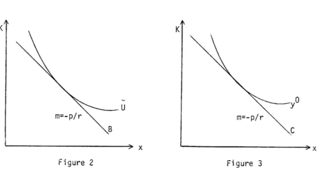
K K 0 U m=-p/r _m=-p/r B C x > x Figure 2 _{Figure 3}

Figure 3 similarly illustrates minimization of isocost, c = p -x + rK, subject to the isoquant determined by y = f(x;K). Tangencies in Figures 2 and 3 represent first-order condition (33).

Hartman's (1979) adapatation of Hausman's (1979) theoretical franework considers precisely the minimization problem: min (p-x + rK) subject to y = f(x;K). Hartman specifies the service demand y as a function of exogenous variables and an efficiency adjusted price for fuel input. His methodology, however, begs the separability issues which allow a formal two-stage consistent budgeting decision to be made.

Our second specialization of the maximization problem (31) assumes that the production function f(x;K) has the form p(K)x. We assume that

p( ) is positive and strictly increasing in K. Note that f now

exhibits a marginal efficiency which is independent of x yet depends

explicitly on the fixed design parameter K. Equation (31) is then

equivalent to:

(35) max U[YJ s.t. (p/p(K))Y < I - H[K]

We may write the indirect utility from (35) as V[I-H(K), p/p(K)] to underscore a direct trade-off between operating and "capital" costs.

If we let H = H[K] and p = p/p(K) then V*[H,P] = V[I-H, p] =

V[I-H(K), p/p(K)] defines the indirect utility when purchase price is H

and service price is p. Figure 4 depicts a level set of the function V*.

H

V T

Figure 4

The curvature and slope of the indifference locus in Figure 4 follow

by application of Roy's identity and the Slutsky equation. Specifically,

dH V2LI-H, p]

(36) ~ - j-H = -Y[I-H, p] < 0

dp V LI-H, p]

wnere the second equality is a consequence of Roy's identity. From equation (36) we have:

(37) ₌

y

dp dp - 1 dp 2 =~-Y₁Y +

where Y1Y + Y2 is equivalent to the Hick's compensated price derivative

of Y[I-H,p] by Slutsky's equation and is therefore nonpositive. The trade-off between purchase price H = H[K] and p = p/p(K) is illustrated by the locus T in Figure 4. The slope of this locus at a point (p, H) is negative if we assume that purchase price is increasing

in the attribute K;

d = $ / dp implies:

dp- dK dK

(38) dH -H'(K) (p(K))2 < 0 as H'(K) > 0.

dp

The curvature of the locus T will depend on the derivatives of the functions H and p and is drawn convex to the origin for illustration only. Note that increasing utility is represented by indifference loci nearer the origin while the feasible price space is determined by the unbounded area above the locus T. It is easy to verify that equating the derivatives (36) and (38) reproduces first-order condition (33) under the maintained assumption f[x; K] = p(K)-x.

Figure 4 suggests a motivation for a dual cost minimization problem which is implicit in the approach of Hirst and Carney (1978):

(39) min (p y0 + H) subject to (p, H) e T p,H

where y denotes a predetermined service level.

One may easily verify that (39) produces the first-order condition (33). The minimization problem (39) is illustrated in Figure 5. We have followed the convention of drawing the locus T concave to the origin. A sufficient condition for this curvature is increasing marginal purchase costs as (38) implies: 2 2 (40) d( = -1 p'IH'2pp' + p ₂ H"] H'p p" _~ < 0_< dK dp p (p') when H"(K) > 0. H T 0 m=-y Figure 5 0

-43-Them examples have illustrated how the consumers durable choice problem can be represented in terms of the optimal choice of technology subject to financial and technological constraints. In the next section we derive conditions under which the separability in utility implied by appliance-production technologies permits a consistent two-stage or "tree" budget program. Under the two-stage budgeting procedure, consumers first determine optimal production service levels and then choose input combina-tions which produce these service levels at minimum cost.