HAL Id: hal-00847778
https://hal.archives-ouvertes.fr/hal-00847778
Submitted on 24 Jul 2013
HAL is a multi-disciplinary open access
archive for the deposit and dissemination of
sci-entific research documents, whether they are
pub-lished or not. The documents may come from
teaching and research institutions in France or
abroad, or from public or private research centers.
L’archive ouverte pluridisciplinaire HAL, est
destinée au dépôt et à la diffusion de documents
scientifiques de niveau recherche, publiés ou non,
émanant des établissements d’enseignement et de
recherche français ou étrangers, des laboratoires
publics ou privés.
Study of a reverberation chamber shape inspired from
chaotic cavities
Kamardine Selemani, Elodie Richalot, Olivier Legrand, Fabrice Mortessagne
To cite this version:
Kamardine Selemani, Elodie Richalot, Olivier Legrand, Fabrice Mortessagne. Study of a reverberation
chamber shape inspired from chaotic cavities. ADVANCED ELECTROMAGNETICS SYMPOSIUM,
Apr 2012, Paris, France. pp.1-5. �hal-00847778�
ADVANCED ELECTROMAGNETICS SYMPOSIUM,AES2012,16–19APRIL 2012,PARIS -FRANCE
Study of a reverberation chamber shape inspired from chaotic cavities
K. Selemani
1*, E. Richalot
1, O. Legrand
2, F. Mortessagne
21
Université Paris-Est, ESYCOM, Marne-la-Vallée, Cité Descartes, 77 454 Marne-la-Vallée, France
2
LPMC, Université de Nice-Sophia Antipolis, Parc Valrose, 06108 Nice cedex 2, France
*
corresponding author, E-mail: selemani@univ-mlv.fr
Abstract
Using the knowledge gained from the wave chaos theory, we present a simple modification of the shape of a reverberation chamber (RC) consisting in inserting a metallic hemisphere on a cavity wall. The presented simulation results show a significant improvement of the field statistical properties, and this without resorting to a mode stirrer.
1.
Introduction
The reverberation chambers, widely used for electromagnetic compatibility studies or antenna characterisation [1], are resonant cavities, usually of rectangular shape and equipped with a stirrer in motion having a complex shape. They are used beyond a minimum frequency from which the fields are statistically isotropic and uniform on a stirrer rotation [2]. As it appears that these statistical requirements correspond to the properties of most modes of a chaotic cavity [3], we propose the use of a chaotic cavity as a reverberation chamber cavity. Indeed, in a chaotic cavity, generic modes (also called ergodic modes, see e.g. [4]) display Gaussian statistics for each component. This statistical behavior can be met at relatively low frequency, thereby leading to statistically isotropic fields and random polarizations even for an unstirred cavity field. Thus, the statistical behavior of each individual ergodic mode might constitute the keystone of an effective reduction of the lowest usable frequency (LUF) in chaotic RCs [5].
The application of the wave chaos theory to electromagnetic systems comes from the analogy between the Schrödinger’s and Helmholtz’s equations in the case of a flat cavity [3]. The Schrödinger equation being scalar, the small cavity height allows the problem reduction to a 2D system with a single field component, so that most studies of chaotic electromagnetic cavities were carried out in 2D [6]. However, a few studies of 3D cavities showed similar properties [7].
Drawing inspiration from a 2D chaotic cavity, we studied a parallelepipedic cavity provided with a metal half-sphere on one wall (fig.1). Its dimensions are: W = 0.785m along (Ox), L = 0.985m along (Oy) and H = 0.995m along (Oz). The hemisphere centred at (31W/42, 3L/4, H) has a radius of R = 0.15m. To evaluate how well the cavity is operating, the distributions of the six field components are examined and compared to those obtained with the cavity without hemisphere.
Figure 1: Cavity with hemisphere and 3D grid for field values extraction.
The simulations are performed using HFSS software, by searching for eigenmodes. The first 232 modes of the empty parallelelipedic cavity as well as the first 232 modes of the cavity loaded by a hemisphere are studied here. Their resonant frequencies vary between 214MHz and 1GHz. To study the field distributions, the values of the three electric field components are recorded for each mode at 1001 points within the cavity volume. These points are taken on a 3D grid included in the cavity (Fig. 1). The distance between two adjacent lines as well as between the 3D grid and the cavity walls is of 50mm. The fields associated to each eigenmode are normalized so that the mean of the square electric field amplitude on the grid points is unitary.
Using simulation results, we first of all focus on the distribution of each field component and determine if a Gaussian law is followed. We then examine the isotropy of the fields associated to the cavity resonances while considering the difference between the standard deviations of each component. Besides, the invariance of the field statistical properties through a rotation of the orthonormal basis is used as a test of the field isotropy.
2.
Field distribution
We first examine the distribution of the three field components for each eigenmode. The orthonormal basis is defined according to the cavity edges as reported in Fig. 1. In a well-operating reverberation chamber, as for the ergodic modes of a chaotic cavity, a normal distribution is expected for each field component.
W=785mm L=985mm
2 We focus, as an example, on the mode at 995MHz, but similar results are obtained with other modes. The mapping of electric field (Fig.2) indicates that the disturbance associated with the hemisphere is global, as the distribution is no longer regular as in the empty cavity (Fig.3). From the 1001 values of the electric field components, we plot the associated histograms as well as the closest normal distributions (for Ex in Figs.2-3).
Visually there is a good agreement between theoretical and empirical laws after the insertion of the hemisphere. The Kolmogorov-Smirnov (KS) at 95% confidence is used to determine whether the two laws are close enough. The answer is 0 if they match and 1 otherwise. In the presented case of Fig. 2, the answer is 0, whereas it is 1 in Fig. 3.
Besides the normal distribution of its components, the field is also required to be isotropic in a well-operating reverberation chamber. We recall that an ergodic field is also isotropic. The field isotropy will be studied in more details in the second part of this paper, but we will first of all eliminate the null components because of the strong degradation of the field isotropy they imply. Whereas the field components that vanish are analytically known for the empty cavity, they have to be determined numerically in the modified cavity. As the field values issued from simulations are never strictly null, a criterion is necessary to decide if a component can be considered or not as null. The criterion of Eq. 1 to consider a field component Ei as null has been
determined by examining the empty cavity simulation results, where the null components are analytically known:
( )
}
{
!(E ),!(E ),!(E ) 0.06 max E ! z y x i (1)where µ(x) indicates the mean value of x.
This special treatment of the null field components is particularly important, as it appears from the simulations of the parallelelipedic cavity, that the KS test answer is 0 for the numerical noise associated to these null components. The latter would indeed appear as being Gaussian distributed if they were not eliminated before applying the KS test. To avoid this problem and show the presence of these modes degrading the field isotropy, the response of the KS test has been modified by associating the value -1 to null components.
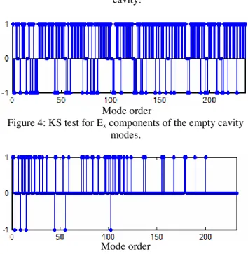
The nullity and KS tests were performed with the first 232 eigenmodes of both cavities. The results obtained for the Ex components of the eigenmodes are given in Fig. 4
for the empty cavity and in Fig. 5 in the presence of the hemisphere. The increase of the number of zero-answers due to the hemisphere insertion clearly appears. Moreover, the Gaussian character of the field improves with increasing frequency in the modified cavity whereas it seems almost completely absent in the empty cavity. The same tests performed on Ey and Ez components of the modes confirm
these remarks.
The results obtained for the three electric field components are summarized in Table I. It can firstly be noticed that, whereas each field component is null for about
28.4% of the modes within the empty cavity, it almost never occurs within the modified cavity. The normal law is widely followed by the field components in the presence of the hemisphere, with a success ratio of the KS test above 72%, whereas the test response is predominantly 1 without the hemisphere.
Figure 2: Electric field amplitude and associated distribution
of Ex component at 995MHz (230 th
mode) for the cavity with an hemisphere
Figure 3: Electric field amplitude and associated distribution of Ex component at 993MHz (230th mode) for the empty
cavity.
Mode order
Figure 4: KS test for Ex components of the empty cavity
modes.
Mode order
Figure 5: KS test for Ex components of the modes obtained
Table 1: Results (%) of the KS test performed on the distribution of the three field components for the 232 resonant
modes of the empty and modified cavities. Null (-1) KS_95%= 1 KS_95% = 0 Ex 23.71 69.4 6.9 Ey 25.43 48.71 25.86 Empty cavity Ez 30.6 38.79 30.6 Ex 2.59 23.28 74.14 Ey 1.72 20.26 78.02 With ! sphere Ez 2.59 24.57 72.84
As for an ergodic mode the three field components are normally distributed, we now define a global homogeneity indicator of the three field properties. It takes the value of -1 if at least one component is null, 0 if each component is non-null and follows a normal distribution, and 1 if no component is null and at least one of the components does not follow a normal distribution
Mode order
Figure 6: Global homogeneity test of all modes, empty cavity
Mode order
Figure 7: Global homogeneity test of all modes, cavity with ! sphere
In the empty cavity, many components are either null or do not follow a normal distribution (Fig.6). In the cavity with a hemisphere null components get extremely rare with increasing frequency; many of them follow a normal distribution (Fig. 7). Table 2 summarizes the results of this global test for all the modes in both cavities. It clearly indicates that the insertion of the hemisphere drastically decreases the number of modes having a null component and increases the number of modes with three normally distributed components.
Table 2: Results (%) of the global homogeneity test performed on the modes
Modes 0 1 -1
Empty cavity 0.42 58.9 40.68 c. with ! sphere 50 43.97 6.03 If the field is isotropic then it presents the same distribution regardless of the chosen orthonormal coordinate system. To verify this property, we modify the first chosen coordinate system of Fig. 1 by performing a rotation of "r=30° about
the Ox axis, of r=20° about the Oy axis and of r=60°
about the Oz axis. The already presented tests are then applied, for each eigenmode of both cavities, to the three components related to this new basis. The results obtained for the global homogeneity indicator of the modified cavity are presented in Fig. 8.
Mode order
Figure 8: Global homogeneity test for the modified cavity, after basis rotation.
The coordinate system rotation eliminates the null components; similarly, the analytical field expressions in the empty cavity indicate that no null component remains in this case. The variation of the number of zero answers from 50% in the initial coordinate system to 63.8% after basis rotation indicates that some modes associated to a zero answer are not ergodic as their field distributions are sensitive to the chosen projection basis.
The modes whose three components are non-null and normally distributed in both coordinate systems, as expected for Gaussian ergodic modes, are presented in Fig. 9. For each mode, if the global homogeneity test takes the value 0 in both coordinate systems, then 0 is indicated, else 1 is associated to this mode. The zero answer is obtained for 38.8% of the modes. As already noticed, the field statistical properties improve with increasing frequency. From the 130th mode, the zero value appears for 73.5% of the modes.
4 Figure 9: Global homogeneity test for the modified cavity,
in both bases.
To further investigate the field isotropy, the standard deviations of the three field components will now be examined.
3.
Standard deviation and field isotropy
The field isotropy implies an equality of the standard deviations of each field component. Therefore, we examine here the standard deviations of the three electric field components for each eigenmode, and use the difference between them as an indicator of the field istropy. The orthonormal basis as defined in Fig. 1 is chosen.The standard deviations are calculated from the components values at the 1001 points of the cavities. Their frequential variations are given in Figs. 10-11.
Figure 10: Standard deviation of Ex, Ey and Ez for the empty
cavity.
Figure 11: Standard deviation of Ex, Ey and Ez for the cavity
with an hemisphere.
We notice a decrease of the standard deviations excursion with increasing frequency in the case of the cavity with a hemisphere, whereas no noticeable evolution appears in the empty cavity. In the latter case, a large number of very small standard deviations are obtained, that correspond to the vanishing of the related field components. These very small values are fewer with the hemisphere. The corresponding null components, very detrimental to the field isotropy, have already be pointed out in Section 2.
The value of 0.577 indicated in Fig. 11 corresponds to an ideal mode whose three components have a zero mean and identical standard deviations. It is expected in a chaotic cavity that the standard deviations fluctuate around this value. Between 700MHz (corresponding to the 76th mode) and 1GHz, the mean values of the standard variations are of 0.54 for Ex, 0.53 for Ey and 0.52 for Ez.
Thus, in the ideal case of an istropic field, the standard deviations of the three electric field components are equal. To evaluate the istropy of the modes, we propose the indicator %& defined in Eq. 2. Its value, comprised between 0 and 1, decreases when the three standard deviations become similar. %& is equal to 1 when one field component vanishes whereas, in the ideal isotropic case, it is vanishing.
(
)
(
)
(
x y z)
(
x y z)
z y x z y x&
&
&
&
&
&
&
&
&
&
&
&
&
,
,
min
,
,
max
,
,
min
,
,
max
+
'
=
%
(2)Figure 12: %& versus frequency for the empty cavity
Figure 13: %& versus frequency for the modified cavity Figure 12 indicates that in the empty parallelelipedic cavity, the variation domain of %& remains globally similar while the frequency increases. On the other hand, %& globally decreases with the frequency in the modified cavity (Fig. 13). The difference between the parameters of both cavities clearly appears after 700MHz: whereas the mean value of %& between 700MHz and 1GHz is of 0.7985 for the empty cavity, it is of 0.5964 in the modified cavity. This is an indication of the improvement of the field isotropy due to the insertion of the hemisphere.
4.
Conclusion
Drawing inspiration from studies developped in the field of wave chaos, a simple modification of the parallelipedic cavity has been proposed with the aim of obtaining homogeneous and isotropic fields. Through simulation results, it has been shown that the ratio of field components following a normal distribution drastically increases after this geometric modification, and that this ratio grows with increasing frequency. The field isotropy has also been discussed from three different points of view. First the modes presenting null components, which are very detrimental to the field isotropy, have been counted, and the reduction of their number in the modified cavity geometry is clearly demonstrated. Then, the invariance of the field statistical properties with respect to the orthonormal basis
has been tested. Finally, the analysis of the standard deviations of the three components and, for each mode, of their dispersion, confirms the same trend.
According to the presented results, the very simple cavity modification we propose permits a considerable improvement of the field statistical properties. The adaptation of this geometrical modification to reverberation chambers could be performed in two ways. The first one consists of inserting a metallic hemisphere within classical reverberation chambers equipped with a stirrer. In the second approach, the hemisphere is considered as a mode-stirrer and moves on the cavity wall. In both approaches, it is expected that the spectral overlap of homogeneous and isotropic modes will lead to better statistical field properties than when the modes do not individually meet the required statistical properties. It would result in the improvement of the reverberation chambers operation and very likely in the decrease of their LUF.
Aknowledgment
The authors thank the french National Research Agency (ANR) for financially supporting the project CAOREV of which this work is a part.
References
[1] P.-S. Kildal, K. Rosengren, J. Byun, J. Lee, “Definition of effective diversity gain and how to measure it in a reverberation chamber”, Microwave and Optical
Technology Letters, Vol. 34, No. 1, July 5 2002, pp. 56-59.
[2] M. O. Hatfield, M. B. Slocum, E. A. Godfrey, and G. J. Freyer, “Investigations to extend the lower frequency limit of reverberation chamber,” in Proc. IEEE Int.
Symp. Electromagn. Compat., Denver, CO, 1998, vol. 1,
pp. 20–23.
[3] H.–J. Stöckman, Quantum Chaos: an introduction, Cambridge University Press (1999).
[4] M.V. Berry, Semiclassical mechanics of Regular and
Irregular Motion, in Chaotic Behaviour of
Deterministic Systems, edited by R.H.G. Helleman and G. Ioss, Les Houches 82, Session XXXVI (North-Holland, Amsterdam, 1983).
[5] L. R. Arnaut, “Operation of electromagnetic reverberation chambers with wave diffractors at relatively low frequencies,” IEEE Trans. Electromagn.
Compat., vol. 43, no. 4, pp. 635–653, Nov. 2001. [6] J. Barthélemy, O. Legrand, F. Mortessagne, “Complete
S-matrix in a microwave cavity at room temperature”, Phys. Rev E, 71, 016205 (2005).
[7] U. Dörr, H. J. Stöckmann, M. Barth, and U. Kuhl, “Scarred and chaotic field distributions in a three-dimensional Sinai-microwave resonator”, Phys. Rev.