HAL Id: hal-00488376
https://hal.archives-ouvertes.fr/hal-00488376
Submitted on 1 Jun 2010
HAL is a multi-disciplinary open access
archive for the deposit and dissemination of
sci-entific research documents, whether they are
pub-lished or not. The documents may come from
teaching and research institutions in France or
abroad, or from public or private research centers.
L’archive ouverte pluridisciplinaire HAL, est
destinée au dépôt et à la diffusion de documents
scientifiques de niveau recherche, publiés ou non,
émanant des établissements d’enseignement et de
recherche français ou étrangers, des laboratoires
publics ou privés.
Orthogonal Group
R. Mahony, Tarek Hamel, Jean-Michel Pflimlin
To cite this version:
R. Mahony, Tarek Hamel, Jean-Michel Pflimlin. Nonlinear Complementary Filters on the Special
Orthogonal Group. IEEE Transactions on Automatic Control, Institute of Electrical and Electronics
Engineers, 2008, 53 (5), pp.1203-1217. �10.1109/TAC.2008.923738�. �hal-00488376�
Non-linear complementary filters on the special
orthogonal group
Robert Mahony, Member, IEEE, Tarek Hamel, Member, IEEE, and Jean-Michel Pflimlin, Member, IEEE
Abstract—This paper considers the problem of obtaining good
attitude estimates from measurements obtained from typical low cost inertial measurement units. The outputs of such systems are characterised by high noise levels and time varying additive biases. We formulate the filtering problem as deterministic observer kinematics posed directly on the special orthogonal group SO(3) driven by reconstructed attitude and angular ve-locity measurements. Lyapunov analysis results for the proposed observers are derived that ensure almost global stability of the observer error. The approach taken leads to an observer that we term the direct complementary filter. By exploiting the geometry of the special orthogonal group a related observer, termed the
passive complementary filter, is derived that decouples the gyro
measurements from the reconstructed attitude in the observer inputs. Both the direct and passive filters can be extended to estimate gyro bias on-line. The passive filter is further developed to provide a formulation in terms of the measurement error that avoids any algebraic reconstruction of the attitude. This leads to an observer on SO(3), termed the explicit complementary filter, that requires only accelerometer and gyro outputs; is suitable for implementation on embedded hardware; and provides good attitude estimates as well as estimating the gyro biases on-line. The performance of the observers are demonstrated with a set of experiments performed on a robotic test-bed and a radio controlled unmanned aerial vehicle.
Index Terms—Complementary filter, nonlinear observer,
atti-tude estimates, special orthogonal group.
I. INTRODUCTION
T
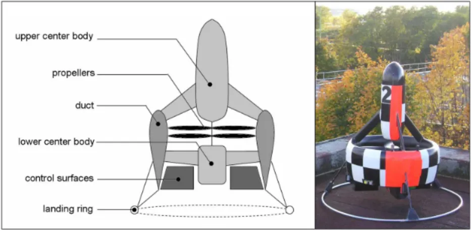
HE recent proliferation of Micro-Electro-Mechanical Systems (MEMS) components has lead to the devel-opment of a range of low cost and light weight inertial measurement units. The low power, light weight and po-tential for low cost manufacture of these units opens up a wide range of applications in areas such as virtual reality and gaming systems, robotic toys, and low cost mini-aerial-vehicles (MAVs) such as the Hovereye (Fig. 1). The signal output of low cost IMU systems, however, is characterised by low-resolution signals subject to high noise levels as well as general time-varying bias terms. The raw signals must be processed to reconstruct smoothed attitude estimates and bias-corrected angular velocity measurements. For many of the low cost applications considered the algorithms need to run on embedded processors with low memory and processing resources.R. Mahony is with Department of Engineering, Australian National Uni-versity, ACT, 0200, Australia. e-mail:[email protected].
T. Hamel is with I3S-CNRS, Nice-Sophia Antipolis, France. e-mail: [email protected].
J.-M. Pflimlin is with Department of Navigation, Dassault Aviation, Saint Cloud, Paris. France. e-mail: [email protected].
Manuscript received November 08, 2006; revised August 03, 2007.
There is a considerable body of work on attitude recon-struction for robotics and control applications (for example [1]–[4]). A standard approach is to use extended stochastic linear estimation techniques [5], [6]. An alternative is to use deterministic complementary filter and non-linear observer design techniques [7]–[9]. Recent work has focused on some of the issues encountered for low cost IMU systems [9]– [12] as well as observer design for partial attitude estimation [13]–[15]. It is also worth mentioning the related problem of fusing IMU and vision data that is receiving recent attention [16]–[19] and the problem of fusing IMU and GPS data [9], [20]. Parallel to the work in robotics and control there is a significant literature on attitude heading reference systems (AHRS) for aerospace applications [21]. An excellent review of attitude filters is given by Crassidis et al. [22]. The recent interest in small low-cost aerial robotic vehicles has lead to a renewed interest in lightweight embedded IMU systems [8], [23]–[25]. For the low-cost light-weight systems considered, linear filtering techniques have proved extremely difficult to apply robustly [26] and linear single-input single-output complementary filters are often used in practice [25], [27]. A key issue is on-line identification of gyro bias terms. This problem is also important in IMU callibration for satellite systems [5], [21], [28]–[31]. An important development that came from early work on estimation and control of satellites was the use of the quaternion representation for the attitude kinematics [30], [32]–[34]. The non-linear observer designs that are based on this work have strong robustness properties and deal well with the bias estimation problem [9], [30]. However, apart from the earlier work of the authors [14], [35], [36] and some recent work on invariant observers [37], [38] there appears to be almost no work that considers the formulation of non-linear attitude observers directly on the matrix Lie-group representation of SO(3).
In this paper we study the design of non-linear attitude observers on SO(3) in a general setting. We term the proposed observers complementary filters because of the similarity of the architecture to that of linear complementary filters (cf. Ap-pendix A), although, for the non-linear case we do not have a frequency domain interpretation. A general formulation of the error criterion and observer structure is proposed based on the Lie-group structure of SO(3). This formulation leads us to propose two non-linear observers on SO(3), termed the
direct complementary filter and passive complementary filter.
The direct complementary filter is closely related to recent work on invariant observers [37], [38] and corresponds (up to some minor technical differences) to non-linear observers proposed using the quaternion representation [9], [30], [32].
Fig. 1. The VTOL MAV HoverEye°c of Bertin Technologies.
We do not know of a prior reference for the passive comple-mentary filter. The passive complecomple-mentary filter has several practical advantages associated with implementation and low-sensitivity to noise. In particular, we show that the filter can be reformulated in terms of vectorial direction measurements such as those obtained directly from an IMU system; a formulation that we term the explicit complementary filter. The explicit complementary filter does not require on-line algebraic reconstruction of attitude, an implicit weakness in prior work on non-linear attitude observers [22] due to the computational overhead of the calculation and poor error characterisation of the constructed attitude. As a result the observer is ideally suited for implementation on embedded hardware platforms. Furthermore, the relative contribution of different data can be preferentially weighted in the observer response, a property that allows the designer to adjust for application specific noise characteristics. Finally, the explicit complementary filter remains well defined even if the data provided is insufficient to algebraically reconstruct the attitude. This is the case, for example, for an IMU with only accelerometer and rate gyro sensors. A comprehensive stability analysis is provided for all three observers that proves local exponential and almost global stability of the observer error dynamics, that is, a stable linearisation for zero error along with global convergence of the observer error for all initial conditions and system trajectories other than on a set of measure zero. Although the principal results of the paper are presented in the matrix Lie group representation of SO(3), the equivalent quaternion representation of the observers are presented in an appendix. The authors recommend that the quaternion representations are used for hardware implementation.
The body of paper consists of five sections followed by a conclusion and two appendices. Section II provides a quick overview of the sensor model, geometry of SO(3) and in-troduces the notation used. Section III details the derivation of the direct and passive complementary filters. The develop-ment here is deliberately kept simple to be clear. Section IV integrates on-line bias estimation into the observer design and provides a detailed stability analysis. Section V develops the
explicit complementary filter, a reformulation of the passive
complementary filter directly in terms of error measurements.
A suite of experimental results, obtained during flight tests of the Hovereye (Fig. 1), are provided in Section VI that demonstrate the performance of the proposed observers. In addition to the conclusion (§VII) there is a short appendix on linear complementary filter design and a second appendix that provides the equivalent quaternion formulation of the proposed observers.
II. PROBLEMFORMULATION ANDNOTATION.
A. Notation and mathematical identities
The special orthogonal group is denoted SO(3). The asso-ciated Lie-algebra is the set of anti-symmetric matrices
so(3) = {A ∈ R3×3| A = −AT}
For any two matrices A, B ∈ Rn×n then the Lie-bracket (or matrix commutator) is [A, B] = AB − BA. Let Ω ∈ R3 then we define Ω×= 0 −Ω3 Ω2 Ω3 0 −Ω1 −Ω2 Ω1 0 .
For any v ∈ R3then Ω×v = Ω×v is the vector cross product. The operator vex : so(3) → R3 denotes the inverse of the Ω× operator
vex (Ω×) = Ω, Ω ∈ R3.
vex(A)×= A, A ∈ so(3)
For any two matrices A, B ∈ Rn×n the Euclidean matrix inner product and Frobenius norm are defined
hhA, Bii = tr(ATB) = n
X
i,j=1
AijBij
||A|| =phhA, Aii =
v u u tXn i,j=1 A2 ij
The following identities are used in the paper (Rv)×= Rv×RT, R ∈ SO(3), v ∈ R3 (v × w)×= [v×, w×] v, w ∈ R3 vTw = hv, wi = 1 2hhv×, w×ii, v, w ∈ R 3 vTv = |v|2=1 2||v×|| 2, v ∈ R3 hhA, v×ii = 0, A = AT ∈ R3, v ∈ R3 tr([A, B]) = 0, A, B ∈ R3×3
The following notation for frames of reference is used • {A} denotes an inertial (fixed) frame of reference. • {B} denotes a body-fixed-frame of reference. • {E} denotes the estimator frame of reference.
Let Pa, Ps denote, respectively, the anti-symmetric and symmetric projection operators in square matrix space
Pa(H) = 1 2(H − H T), P s(H) = 1 2(H + H T).
Let (θ, a) (|a| = 1) denote the angle-axis coordinates of
R ∈ SO(3). One has [39]:
R = exp(θa×), log(R) = θa×
cos(θ) = 1
2(tr(R) − 1), Pa(R) = sin(θ)a×.
For any R ∈ SO(3) then 3 ≥ tr(R) ≥ −1. If tr(R) = 3 then
θ = 0 in angle-axis coordinates and R = I. If tr(R) = −1
then θ = ±π, R has real eigenvalues (1, −1, −1), and there exists an orthogonal diagonalising transformation U ∈ SO(3) such that U RUT = diag(1, −1, −1).
For any two signals x(t) : R → Mx, y(t) : R → My are termed asymptotically dependent if there exists a non-degenerate function ft : Mx× My → R and a time T such that for any t > T
ft(x(t), y(t)) = 0.
By the term non-degenerate we mean that the Hessian of ft at any point (x, y) is full rank. The two signals are termed
asymptotically independent if for any non-degenerate ft and any T there exists t1> T with ft(x(t1), y(t1)) 6= 0.
B. Measurements
The measurements available from a typical inertial mea-surement unit are 3-axis rate gyros, 3-axis accelerometers and 3-axis magnetometers. The reference frame of the strap down IMU is termed the body-fixed-frame {B}. The inertial frame is denoted {A}. The rotation R = ABR denotes the relative
orientation of {B} with respect to {A}.
Rate Gyros: The rate gyro measures angular velocity of {B}
relative to {A} expressed in the body-fixed-frame of reference {B}. The error model used in this paper is
Ωy= Ω + b + µ ∈ R3
where Ω ∈ {B} denotes the true value, µ denotes additive measurement noise and b denotes a constant (or slowly time-varying) gyro bias.
Accelerometer: Denote the instantaneous linear acceleration
of {B} relative to {A}, expressed in {A}, by ˙v. An ideal accelerometer, ‘strapped down’ to the body-fixed-frame
{B}, measures the instantaneous linear acceleration of {B} minus the (conservative) gravitational acceleration
field g0 (where we consider g0 expressed in the inertial
frame {A}), and provides a measurement expressed in the body-fixed-frame {B}. In practice, the output a from a MEMS component accelerometer has added bias and noise,
a = RT( ˙v − g0) + ba+ µa,
where ba is a bias term and µa denotes additive measure-ment noise. Normally, the gravitational field g0= |g0|e3
where |g0| ≈ 9.8 dominates the value of a for low
frequency response. Thus, it is common to use
va= a
|a| ≈ −R
Te
3
as a low-frequency estimate of the inertial z-axis ex-pressed in the body-fixed-frame.
Magnetometer: The magnetometers provide measurements of
the magnetic field
m = RT Am + B
m+ µb
where Am is the Earths magnetic field (expressed in
the inertial frame), Bm is a body-fixed-frame expres-sion for the local magnetic disturbance and µb denotes measurement noise. The noise µb is usually quite low for magnetometer readings, however, the local magnetic disturbance can be very significant, especially if the IMU is strapped down to an MAV with electric motors. Only the direction of the magnetometer output is relevant for attitude estimation and we will use a vectorial measure-ment
vm= m
|m|
in the following development
The measured vectors va and vm can be used to construct an instantaneous algebraic measurement of the rotation ABR : {B} → {A} Ry= arg min R∈SO(3) ¡ λ1|e3− Rva|2+ λ2|v∗m− Rvm|2 ¢ ≈A BR
where vm∗ is the inertial direction of the magnetic field in the locality where data is acquired. The weights λ1 and λ2
are chosen depending on the relative confidence in the sensor outputs. Due to the computational complexity of solving an op-timisation problem the reconstructed rotation is often obtained in a suboptimal manner where the constraints are applied in sequence; that is, two degrees of freedom in the rotation matrix are resolved using the acceleration readings and the final degree of freedom is resolved using the magnetometer. As a consequence, the error properties of the reconstructed attitude
Ry can be difficult to characterise. Moreover, if either mag-netometer or accelerometer readings are unavailable (due to local magnetic disturbance or high acceleration manoeuvres) then it is impossible to resolve the vectorial measurements into a unique instantaneous algebraic measurement of attitude.
C. Error criteria for estimation on SO(3)
Let ˆR denote an estimate of the body-fixed rotation matrix R = A
BR. The rotation ˆR can be considered as coordinates for the estimator frame of reference {E}. It is also associated with the frame transformation
ˆ
R =A
ER : {E} → {A}.ˆ
The goal of attitude estimate is to drive ˆR → R. The estimation error used is the relative rotation from body-fixed-frame {B} to the estimator body-fixed-frame {E}
˜
R := ˆRTR, R =˜ E
BR : {B} → {E}.˜ (1) The proposed observer design is based on Lyapunov stabil-ity analysis. The Lyapunov functions used are inspired by the cost function Etr := 1 4kI3− ˜Rk 2= 1 4tr ³ (I3− ˜R)T(I3− ˜R) ´ =1 2tr(I3− ˜R) (2)
One has that
Etr =
1
2tr(I − ˜R) = (1 − cos(θ)) = 2 sin(θ/2)
2. (3)
where θ is the angle associated with the rotation from {B} to frame {E}. Thus, driving Eq. 2 to zero ensures that θ → 0.
III. COMPLEMENTARY FILTERS ONSO(3)
In this section, a general framework for non-linear comple-mentary filtering on the special orthogonal group is introduced. The theory is first developed for the idealised case where R(t) and Ω(t) are assumed to be known and used to drive the filter dynamics. Filter design for real world signals is considered in later sections.
The goal of attitude estimation is to provide a set of dynamics for an estimate ˆR(t) ∈ SO(3) to drive the error
rotation (Eq. 1) ˜R(t) → I3. The kinematics of the true system
are
˙
R = RΩ×= (RΩ)×R (4) where Ω ∈ {B}. The proposed observer equation is posed directly as a kinematic system for an attitude estimate ˆR on
SO(3). The observer kinematics include a prediction term
based on the Ω measurement and an innovation or correction term ω := ω( ˜R) derived from the error ˜R. The general form proposed for the observer is
˙ˆ
R = (RΩ + kPRω)ˆ ×R,ˆ R(0) = ˆˆ R0, (5)
where kP > 0 is a positive gain. The term (RΩ + kPRω) ∈ˆ
{A} is expressed in the inertial frame. The body-fixed-frame
angular velocity is mapped back into the inertial frame AΩ =
RΩ. If no correction term is used (kPω ≡ 0) then the error rotation ˜R is constant, ˙˜ R = ˆRT(RΩ)T ×R + ˆRT(RΩ)×R = ˆRT(−(RΩ) ×+ (RΩ)×) R = 0. (6) The correction term ω := ω( ˜R) ∈ {E} is considered to be in the estimator frame of reference. It can be thought of
as a non-linear approximation of the error between R and
ˆ
R as measured from the frame of reference associated with
ˆ
R. In practice, it will be implemented as an error between a
measured estimate Ry of R and the estimate ˆR.
The goal of the observer design is to find a simple expres-sion for ω that leads to robust convergence of ˜R → I. In prior
work [35], [36] the authors introduced the following correction term
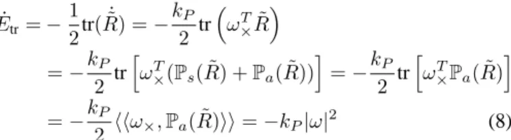
ω := vex(Pa( ˜R)) = vex(Pa( ˆRTRy)) (7) This choice leads to an elegant Lyapunov analysis of the filter stability. Differentiating the storage function Eq. 2 along trajectories of Eq. 5 yields
˙ Etr= − 1 2tr(R) = −˙˜ kP 2 tr ³ ωT ×R˜ ´ = −kP 2 tr h ωT×(Ps( ˜R) + Pa( ˜R)) i = −kP 2 tr h ωT×Pa( ˜R) i = −kP 2 hhω×, Pa( ˜R)ii = −kP|ω| 2 (8)
In Mahony et al. [35] a local stability analysis of the filter dynamics Eq. 5 is provided based on this derivation. In Section IV a global stability analysis for these dynamics is provided. We term the filter Eq. 5 a complementary filter on SO(3) since it recaptures the block diagram structure of a classical complementary filter (cf. Appendix A). In Figure 2: The ‘ ˆRT’
ˆ R k ˆ RTR Ω
Maps angular velocity
Maps angular velocity
˜ R + + Inverse operation on SO(3) System Maps error ˜R R R ˙ˆ R= A ˆR (RΩ)× on SO(3) Difference operation
into correct frame of reference
onto TI SO(3).
onto TI SO(3). kinematics A
ˆ RT
RΩ
Pa( ˜R)
Fig. 2. Block diagram of the general form of a complementary filter on SO(3).
operation is an inverse operation on SO(3) and is equivalent to a ‘−’ operation for a linear complementary filter. The ‘ ˆRTR
y’
operation is equivalent to generating the error term ‘y − ˆx’.
The two operations Pa( ˜R) and (RΩ)× are maps from error space and velocity space into the tangent space of SO(3); operations that are unnecessary on Euclidean space due to the identification TxRn ≡ Rn. The kinematic model is the Lie-group equivalent of a first order integrator.
To implement the complementary filter it is necessary to map the body-fixed-frame velocity Ω into the inertial frame. In practice, the ‘true’ rotation R is not available and an estimate of the rotation must be used. Two possibilities are considered:
direct complementary filter: The constructed attitude Ry is used to map the velocity into the inertial frame
˙ˆ
R = (RyΩy+ kPRω)ˆ ×R.ˆ
A block diagram of this filter design is shown in Figure 3. This approach can be linked to observers documented
in earlier work [30], [32] (cf. Appendix B). The approach has the advantage that it does not introduce an additional feedback loop in the filter dynamics, however, high frequency noise in the reconstructed attitude Ry will enter into the feed-forward term of the filter.
ˆ R k ˆ RT + + ˙ˆ R= A ˆR (RyΩy)× A Ωy Ry RyΩy ˜ R ˆ RTRy Pa( ˜R)
Fig. 3. Block diagram of the direct complementary filter on SO(3). passive complementary filter: The filtered attitude ˆR is used
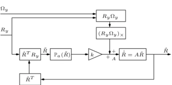
in the predictive velocity term
˙ˆ
R = ( ˆRΩy+ kPRω)ˆ ×R.ˆ (9) A block diagram of this architecture is shown in Figure 4. The advantage lies in avoiding corrupting the predictive angular velocity term with the noise in the reconstructed pose. However, the approach introduces a secondary feedback loop in the filter and stability needs to be proved. ˆ R k + + ˆ RTRy R˙ˆ= A ˆR Ry Ωy ˜ R ( ˆRΩy)× ˆ RΩy ˆ RT A Pa( ˜R)
Fig. 4. Block diagram of the passive complementary filter on SO(3).
A key observation is that the Lyapunov stability analysis in Eq. 8 is still valid for Eq. 9, since
˙ Etr= − 1 2tr(R) = −˙˜ 1 2tr(−(Ω + kPω)×R + ˜˜ RΩ×) = −1 2tr([ ˜R, Ω×]) − kP 2 tr(ω T ×R) = −k˜ P|ω|2, using the fact that the trace of a commutator is zero, tr([ ˜R, Ω×]) = 0. The filter is termed a passive complimentary filter since the cross coupling between Ω and ˜R does not
contribute to the derivative of the Lyapunov function. A global stability analysis is provided in Section IV.
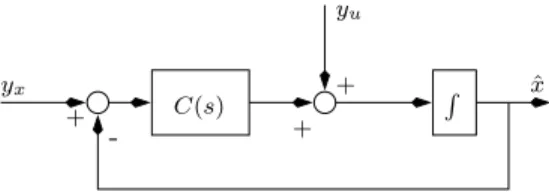
There is no particular theoretical advantage to either the direct or the passive filter architecture in the case where exact measurements are assumed. However, it is straightforward to see that the passive filter (Eq. 9) can be written
˙ˆ
R = ˆR(Ω×+ kPPa( ˜R)). (10) This formulation suppresses entirely the requirement to repre-sent Ω and ω = kPPa( ˜R) in the inertial frame and leads to
the architecture shown in Figure 5. The passive complementary filter avoids coupling the reconstructed attitude noise into the predictive velocity term of the observer, has a strong Lyapunov stability analysis, and provides a simple and elegant realisation that will lead to the results in Section V.
˙ˆ R= ˆRA Rˆ k Ωy Ry ˆ RTR (Ω)× ˆ RT Pa( ˜R)
Fig. 5. Block diagram of the simplified form of the passive complementary filter.
IV. STABILITYANALYSIS
In this section, the direct and passive complementary filters on SO(3) are extended to provide on-line estimation of time-varying bias terms in the gyroscope measurements and global stability results are derived. Preliminary results were published in [35], [36].
For the following work it is assumed that a reconstructed rotation Ry and a biased measure of angular velocity Ωy are available
Ry ≈ R, valid for low frequencies, (11a)
Ωy ≈ Ω + b for constant bias b. (11b) The approach taken is to add an integrator to the compensator term in the feedback equation of the complementary filter.
Let kP, kI > 0 be positive gains and define
Direct complementary filter with bias correction:
˙ˆ R = ³ Ry(Ωy− ˆb) + kPRωˆ ´ × ˆ R, R(0) = ˆˆ R0, (12a) ˙ˆb = −kIω, ˆb(0) = ˆb0, (12b) ω = vex(Pa( ˜R)), R = ˆ˜ RTRy. (12c)
Passive complementary filter with bias correction:
˙ˆ R = ˆR³Ωy− ˆb + k Pω ´ ×, ˆ R(0) = ˆR0, (13a) ˙ˆb = −kIω, ˆb(0) = ˆb0, (13b) ω = vex(Pa( ˜R)), R = ˆ˜ RTRy. (13c) The non-linear stability analysis is based on the idea of an adaptive estimate for the unknown bias value.
Theorem 4.1: [Direct complementary filter with bias correction.] Consider the rotation kinematics Eq. 4 for a
time-varying R(t) ∈ SO(3) and with measurements given by Eq. 11. Let ( ˆR(t), ˆb(t)) denote the solution of Eq. 12. Define error variables ˜R = ˆRTR and ˜b = b − ˆb. Define
U ⊆ SO(3) × R3 by U = n ( ˜R, ˜b) tr( ˜R) = −1, Pa(˜b×R) = 0˜ o . (14) Then:
1) The set U is forward invariant and unstable with respect to the dynamic system Eq. 12.
2) The error ( ˜R(t), ˜b(t)) is locally exponentially stable to
(I, 0).
3) For almost all initial conditions ( ˜R0, ˜b0) 6∈ U the
trajec-tory ( ˆR(t), ˆb(t)) converges to the trajectory (R(t), b).
Proof: Substituting for the error model (Eq. 11), Equation
12a becomes ˙ˆ R =³R(Ω + ˜b) + kPRωˆ ´ × ˆ R.
Differentiating ˜R it is straightforward to verify that
˙˜
R = −kPω×R − ˜b˜ ×R.˜ (15)
Define a candidate Lyapunov function by
V = 1 2tr(I3− ˜R) + 1 2kI |˜b|2= E tr+ 1 2kI |˜b|2 (16)
Differentiating V one obtains
˙ V = −1 2tr(R) −˙˜ 1 kI˜b T˙ˆb =1 2tr ³ kPω×R + ˜b˜ ×R˜ ´ − 1 kI h˜b,˙ˆbi =−kP 2 hhω×, Pa( ˜R) + Ps( ˜R)ii −1 2hh˜b×, Pa( ˜R) + Ps( ˜R)ii − 1 kI h˜b,˙ˆbi
= −kPhω, vex(Pa( ˜R))i − h˜b, vex(Pa( ˜R)i − 1
kIh˜b,˙ˆbi Substituting for ˙ˆb and ω (Eqn’s 12b and 12c) one obtains
˙
V = −kP|ω|2= −kP|vexPa( ˜R)|2 (17) Lyapunov’s direct method ensures that ω converges asymptoti-cally to zero [40]. Recalling that ||Pa( ˜R)|| =
√
2 sin(θ), where (θ, a) denotes the angle-axis coordinates of ˜R. It follows that ω ≡ 0 implies either ˜R = I, or log( ˜R) = πa× for |a| = 1. In the second case one has the condition tr( ˜R) = −1. Note
that ω = 0 is also equivalent to requiring ˜R = ˜RT to be symmetric.
It is easily verified that (I, 0) is an isolated equilibrium of the error dynamics Eq. 18.
From the definition of U one has that ω ≡ 0 on U. We will prove that U is forward invariant under the filter dynamics Eqn’s 12. Setting ω = 0 in Eq. 15 and Eq. 12b yields
˙˜
R = −˜b×R,˜ ˙ˆb = 0. (18) For initial conditions ( ˜R0, ˜b0) = ( ˜R0, ˜b0) ∈ U the solution of
Eq. 18 is given by
˜
R(t) = exp(−t˜b×) ˜R0, ˜b(t) = ˜b0, ( ˜R0, ˜b0) ∈ U.
(19)
We verify that Eq. 19 is also a general solution of Eqn’s 15 and 12b. Differentiating tr( ˜R) yields
d dttr( ˜R) = −tr(˜b×exp(−t˜b×) ˜R0) = tr à exp(−t˜b×)(˜b× ˜ R0+ ˜R0˜b×) 2 ! = tr³exp(−t˜b×)Pa(˜b×R˜0) ´ = 0,
where the second line follows since ˜b× commutes with
exp(˜b×) and the final equality is due to the fact that
Pa(˜b×R˜0) = 0, a consequence of the choice of initial
conditions ( ˜R0, ˜b0) ∈ U. It follows that tr( ˜R(t)) = −1 on
solution of Eq. 19 and hence ω ≡ 0. Classical uniqueness results verify that Eq. 19 is a solution of Eqn’s 15 and 12b. It remains to show that such solutions remain in U for all time. The condition on ˜R is proved above. To see that Pa(˜b×R) ≡ 0˜ we compute
d
dtPa(˜b×R) = −P˜ a(˜b
2
×R) = −P˜ a(˜b×R˜b˜ T×) = 0 as ˜R = ˜RT. This proves that U is forward invariant.
Applying LaSalle’s principle to the solutions of Eq. 12 it follows that either ( ˜R, ˜b) → (I, 0) asymptotically or ( ˜R, ˜b) →
( ˜R∗(t), ˜b0) where ( ˜R∗(t), ˜b0) ∈ U is a solution of Eq. 18.
To determine the local stability properties of the invariant sets we compute the linearisation of the error dynamics. We will prove exponential stability of the isolated equilibrium point (I, 0) first and then return to prove instability of the set U. Define x, y ∈ R3 as the first order approximations of
˜
R and ˜b around (I, 0)
˜
R ≈ (I + x×), x×∈ so(3) (20a)
˜b = −y. (20b)
The sign change in Eq. 20b simplifies the analysis of the linearisation. Substituting into Eq. 15, computing ˙˜b and dis-carding all terms of quadratic or higher order in (x, y) yields
d dt à x y ! = à −kPI3 I3 −kII3 0 ! à x y ! (21) For positive gains kP, kI > 0 the linearised error system is strictly stable. This proves part ii) of the theorem statement.
To prove that U is unstable, we use the quaternion formu-lation (see Appendix B). Using Eq. 49, the error dynamics of the quaternion ˜q = (˜s, ˜v) associated to the rotation ˜R is given
by ˙˜s = 1 2(kPs|˜˜v| 2+ ˜vT˜b), (22a) ˙˜b = kIs˜˜v, (22b) ˙˜v = −1 2(˜s(˜b + kPs˜˜v) + ˜b × ˜v), (22c)
It is straightforward to verify that the invariant set associated to the error dynamics is characterised by
Define y = ˜bTv, then an equivalent characterisation of U is˜ given by (˜s, y) = (0, 0). We study the stability properties
of the equilibrium (0, 0) of (˜s, y) evolving under the filter
dynamics Eq. 12. Combining Eq. 22c and 22b, one obtains the following dynamics for ˙y
˙y = ˜vT˙˜b + ˜bT˙˜v
= kI˜s|˜v|2−12s|˜b|˜ 2−12kPs˜2y Linearising around small values of (˜s, y) one obtains
à ˙˜s ˙y ! = à 1 2kP 1 2 kI−12|˜b0|2 0 ! à ˜ s y !
Since KP and KI are positive gains it follows that the lineari-sation is unstable around the point (0, 0) and this completes the proof of part i).
The linearisation of the dynamics around the unstable set is either strongly unstable (for large values of |˜b0|2) or hyperbolic
(both positive and negative eigenvalues). Since ˜b0depends on
the initial condition then there there will be trajectories that converge to U along the stable centre manifold [40] associated with the stable direction of the linearisation. From classical centre manifold theory it is known that such trajectories are measure zero in the overall space. Observing in addition that
U is measure zero in SO(3) × R3proves part iii) and the full proof is complete.
The direct complimentary filter is closely related to quater-nion based attitude filters published over the last fifteen years [9], [30], [32]. Details of the similarities and differences is given in Appendix B where we present quaternion versions of the filters we propose in this paper. Apart from the formulation directly on SO(3), the present paper extends earlier work by proposing globally defined observer dynamics and a full global analysis. To the authors best understanding, all prior published algorithms depend on a sgn(θ) term that is discon-tinuous on U (Eq. 14). Given that the observers are not well defined on the set U the analysis for prior work is necessarily non-global. However, having noted this, the recent work of Thienel et al. [30] provides an elegant powerful analysis that transforms the observer error dynamics into a linear time-varying system (the transformation is only valid on a domain on SO(3) × R3− U) for which global asymptotic stability is
proved. This analysis provides a global exponential stability under the assumption that the observer error trajectory does not intersect U. In all practical situations the two approaches are equivalent.
The remainder of the section is devoted to proving an anal-ogous result to Theorem 4.1 for the passive complementary filter dynamics. In this case, it is necessary to deal with non-autonomous terms in the error dynamics due to passive coupling of the driving term Ω into the filter error dynamics. Interestingly, the non-autonomous term acts in our favour to disturb the forward invariance properties of the set U (Eq. 14) and reduce the size of the unstable invariant set.
Theorem 4.2: [Passive complementary filter with bias correction.] Consider the rotation kinematics Eq. 4 for a
time-varying R(t) ∈ SO(3) and with measurements given by Eq. 11. Let ( ˆR(t), ˆb(t)) denote the solution of Eq. 13. Define
error variables ˜R = ˆRTR and ˜b = b − ˆb. Assume that Ω(t) is a bounded, absolutely continuous signal and that the pair of signals (Ω(t), ˜R) are asymptotically independent (see §II-A).
Define U0⊆ SO(3) × R3 by U0= n ( ˜R, ˜b) tr( ˜R) = −1, ˜b = 0 o . (23) Then:
1) The set U0is forward invariant and unstable with respect
to the dynamic system 13.
2) The error ( ˜R(t), ˜b(t)) is locally exponentially stable to
(I, 0).
3) For almost all initial conditions ( ˜R0, ˜b0) 6∈ U0 the
tra-jectory ( ˆR(t), ˆb(t)) converges to the trajectory (R(t), b).
Proof: Substituting for the error model (Eq. 11) in Eqn’s
13 and differentiating ˜R, it is straightforward to verify that
˙˜
R = [ ˜R, Ω×] − kPω×R − ˜b˜ ×R,˜ (24a)
˙˜b = kIω (24b) The proof proceeds by differentiating the Lyapunov-like func-tion Eq. 16 for solufunc-tions of Eq. 13. Following an analogous derivation to that in Theorem 4.1, but additionally exploiting the cancellation tr([ ˜R, Ω×]) = 0, it may be verified that
˙
V = −kP|ω|2= −kP|vex(Pa( ˜R))|2
where V is given by Eq. 16. This bounds V (t) ≤ V (0), and it follows ˜b is bounded. LaSalle’s principle cannot be applied
directly since the dynamics Eq. 24a are not autonomous. The function ˙V is uniformly continuous since the derivative
¨
V = −kPPa( ˜R)T
³
Pa([ ˜R, Ω×]) − Pa((kPω − ˜b)×) ˜R
´
is uniformly bounded. Applying Barbalat’s lemma proves asymptotic convergence of ω = vex(Pa( ˜R)) to zero.
Direct substitution shows that ( ˜R, ˜b) = (I, 0) is an equilib-rium point of Eq. 24. Note that U0 ⊂ U (Eq. 14) and hence
ω ≡ 0 on U (Th. 4.1). For ( ˜R, ˜b) ∈ U0 the error dynamics
Eq. 24 become
˙˜
R = [ ˜R, Ω×], ˙˜b = 0.
The solution of this ordinary differential equation is given by
˜
R(t) = exp(−A(t)) ˜R0exp(A(t)), A(t) =
Z t
0
Ω×dτ. Since A(t) is anti-symmetric for all time then exp(−A(t)) is orthogonal and since exp(−A(t)) = exp(A(t))T it follows ˜R is symmetric for all time. It follows that U0is forward invariant
under the filter dynamics Eq. 13. We prove by contradiction that U0⊂ U is the largest forward invariant set of the
closed-loop dynamics Eq. 13 such that ω ≡ 0. Assume that there exits ( ˜R0, ˜b0) ∈ U − U0 such that ( ˜R(t), ˜b(t)) remains in U
for all time. One has that Pa(˜b×R) = 0 on this trajectory.˜ Consequently, d dtPa(˜b×R) = P˜ a(˜b×[ ˜R, Ω×]) − P(˜b×Rb˜ T ×) = Pa(˜b×[ ˜R, Ω×]) = −1 2 ³ (˜b × Ω)×R + ˜˜ R(˜b × Ω)× ´ = 0, (25)
where we have used
2Pa(˜b×R) = ˜b˜ ×R + ˜˜ R˜b×= 0, (26) several times in simplifying expressions. Since (Ω(t), ˜R(t)) are asymptotically independent then the relationship Eq. 25 must be degenerate. This implies that there exists a time T such that for all t > T then ˜b(t) ≡ 0 and contradicts the assumption.
It follows that either ( ˜R, ˜b) → (I, 0) asymptotically or
( ˜R, ˜b) → ( ˜R∗(t), 0) ∈ U0.
Analogously to Theorem 4.1 the linearisation of the error dynamics (Eq. 24) at (I, 0) is computed. Let ˜R ≈ I + x× and ˜b ≈ −y for x, y ∈ R3. The linearised dynamics are the time-varying linear system
d dt à x y ! = à −kPI3− Ω(t)× I3 −kII3 0 ! à x y !
Let |Ωmax| denote the magnitude bound on Ω and choose α2> 0, α1> α2(|Ωmax|2+ kI) kP , α1+ kPα2 kI < α3< α1+ kPα2 kI + |Ωmax|α2 kI Set P, Q to be matrices P = µ α1I3 −α2I3 −α2I3 α3I3 ¶ , Q = µ kPα1− α2kI −α2|Ωmax| −α2|Ωmax| α2 ¶ (27) It is straightforward to verify that P and Q are positive definite matrices given the constraints on {α1, α2, α3}.
Con-sider the cost function W = 12ξTP ξ, with ξ = (x, y)T. Differentiating W yields
˙
W = − (kPα1− α2kI)|x|2− α2|y|2
+ yTx(α
1+ kPα2− α3kI) + α2yT(Ω × x) (28)
It is straightforward to verify that
d dt ¡ ξTP ξ¢≤ −2(|x|, |y|) Q Ã |x| |y| ! .
This proves exponential stability of the linearised system at
(I, 0).
The linearisation of the error dynamics on a trajectory in
U0 are also time varying and it is not possible to use the
argument from Theorem 4.1 to prove instability. However, note that V ( ˜R∗, ˜b∗) = 2 for all ( ˜R∗, ˜b∗) ∈ U0. Moreover,
any neighbourhood of a point ( ˜R∗, ˜b∗) ∈ U0 within the set
SO(3) × R3 contains points ( ˜R, ˜b) such the V ( ˜R, ˜b) < 2.
Trajectories with these initial conditions cannot converge to U0
due to the decrease condition derived earlier, and it follows that
U0 is unstable. Analogous to Theorem 4.1 it is still possible
that a set of measure zero initial conditions, along with very specific trajectories Ω(t), such that the resulting trajectories converge to to U0. This proves part iii) and completes the
proof.
Apart from the expected conditions inherited from Theo-rem 4.1 the key assumption in TheoTheo-rem 4.2 is the indepen-dence of Ω(t) from the error signal ˜R. The perturbation of the
passive dynamics by the independent driving term Ω provides a disturbance that ensures that the adaptive bias estimate converges to the true gyroscopes’ bias, a particularly useful property in practical applications.
V. EXPLICIT ERROR FORMULATION OF THE PASSIVE COMPLEMENTARY FILTER
A weakness of the formulation of both the direct and passive and complementary filters is the requirement to reconstruct an estimate of the attitude, Ry, to use as the driving term for the error dynamics. The reconstruction cannot be avoided in the direct filter implementation because the reconstructed attitude is also used to map the velocity into the inertial frame. In this section, we show how the passive complementary filter may be reformulated in terms of direct measurements from the inertial unit.
Let v0i ∈ {A}, i = 1, . . . , n, denote a set of n known
inertial directions. The measurements considered are body-fixed-frame observations of the fixed inertial directions
vi= RTv0i+ µi, vi∈ {B} (29) where µi is a noise process. Since only the direction of the measurement is relevant to the observer we assume that |v0i| =
1 and normalise all measurements to ensure |vi| = 1. Let ˆR be an estimate of R. Define
ˆ
vi= ˆRTv0i
to be the associated estimate of vi. For a single direction vi, the error considered is
Ei= 1 − cos(∠vi, ˆvi) = 1 − hvi, ˆvii which yields
Ei = 1 − tr( ˆRTv0iv0iTR) = 1 − tr( ˜RRTv0ivT0iR)
For multiple measures vi the following cost function is con-sidered Emes= n X i=1 kiEi= n X i=1 ki− tr( ˜RM ), ki> 0, (30) where M = RTM 0R with M0= n X i=1 kiv0ivT0i (31)
Assume linearly independent inertial direction {v0i} then the
matrix M is positive definite (M > 0) if n ≥ 3. For n = 2 then M is positive semi-definite with one eigenvalue zero. The weights ki > 0 are chosen depending on the relative confidence in the measurements vi. For technical reasons in the proof of Theorem 5.1 we assume additionally that the weights
kiare chosen such that M0has three distinct eigenvalues λ1>
λ2> λ3.
Theorem 5.1: [Explicit complementary filter with bias correction.] Consider the rotation kinematics Eq. 4 for a
time-varying R(t) ∈ SO(3) and with measurements given by Eqn’s 29 and 11b. Assume that there are two or more, (n ≥ 2) vectorial measurements vi available. Choose ki > 0 such
that M0 (defined by Eq. 31) has three distinct eigenvalues.
Consider the filter kinematics given by
˙ˆ R = ˆR ³ (Ωy− ˆb) ×+ kP(ωmes)× ´ , R(0) = ˆˆ R0 (32a) ˙ˆb = −kIωmes (32b) ωmes:= n X i=1 kivi× ˆvi, ki> 0. (32c) and let ( ˆR(t), ˆb(t)) denote the solution of Eqn’s 32. Assume that Ω(t) is a bounded, absolutely continuous signal and that the pair of signals (Ω(t), ˜RT) are asymptotically independent (see §II-A). Then:
1) There are three unstable equilibria of the filter charac-terised by ( ˆR∗i, ˆb∗i) = ¡ U0DiU0TR, b ¢ , i = 1, 2, 3,
where D1 = diag(1, −1, −1), D2 = diag(−1, 1, −1)
and D3 = diag(−1, −1, 1) are diagonal matrices with
entries as shown and U0 ∈ SO(3) such that M0 =
U0ΛU0T where Λ = diag(λ1, λ2, λ3) is a diagonal
matrix.
2) The error ( ˜R(t), ˜b(t)) is locally exponentially stable to
(I, 0).
3) For almost all initial conditions ( ˜R0, ˜b0) 6= ( ˆRT∗iR, b),
i = 1, . . . , 3, the trajectory ( ˆR(t), ˆb(t)) converges to the
trajectory (R(t), b).
Proof: Define a candidate Lyapunov-like function by
V = n X i=1 ki− tr( ˜RM ) + 1 kI˜b 2= E mes+ 1 kI˜b 2
The derivative of V is given by
˙ V = − tr³RM + ˜˙˜ R ˙M´− 2 kI˜b T˙ˆb = −tr ³ [ ˜RM, Ω×] − (˜b + kPωmes)×RM˜ ´ − 2 kI˜b T˙ˆb
Recalling that the trace of a commutator is zero, the derivative of the candidate Lyapunov function can be simplified to obtain
˙ V = kPtr ³ (ωmes)×Pa( ˜RM ) ´ +tr µ ˜b× µ Pa( ˜RM ) − 1 kI˙ˆb× ¶¶ (33) Recalling the identities in Section II-A one may write ωmes
as (ωmes)×= n X i=1 ki 2(ˆviv T i − vivˆiT) = Pa( ˜RM ) (34) Introducing the expressions of ωmesinto the time derivative
of the Lyapunov-like function V , Eq. 33, one obtains
˙
V = −kP||Pa( ˜RM )||2.
The Lyapunov-like function derivative is negative semi-definite ensuring that ˜b is bounded. Analogous to the proof of Theorem 4.2, Barbalat’s lemma is invoked to show that
Pa( ˜RM ) tends to zero asymptotically. Thus, for ˙V = 0 one has
˜
RM = M ˜RT. (35)
We prove next Eq. 35 implies either ˜R = I or tr( ˜R) = −1.
Since ˜R is a real matrix, the eigenvalues and eigenvectors
of ˜R verify
˜
RTxk = λkxk and xHkR = λ˜ Hk xHk (36) where λHk (for k = 1 . . . 3) represents the complex conjugate of the eigenvalue λk and xHk represents the Hermitian trans-pose of the eigenvector xkassociated to λk. Combining Eq. 35 and Eq. 36, one obtains
xHkRM x˜ k = λHk xHk M xk
xH
kM ˜RTxk = λkxkHM xk = λHk xHk M xk
Note that for n ≥ 3, M > 0 is positive definite and
xH
kM xk > 0, ∀k = {1, 2, 3}. One has λk = λHk for all k. In the case when n = 2, it is simple to verify that two of the three eigenvalues are real. It follows that all three eigenvalues of ˜R are real since complex eigenvalues must come in complex conjugate pairs. The eigenvalues of an orthogonal matrix are of the form
eig( ˜R) = (1, cos(θ) + i sin(θ), cos(θ) − i sin(θ)),
where θ is the angle from the angle-axis representation. Given that all the eigenvalues are real it follows that θ = 0 or θ =
±π. The first possibility is the desired case ( ˜R, ˜b) = (I, 0).
The second possibility is the case where tr( ˜R) = −1.
When ωmes ≡ 0 then Eqn’s 32 and Eqn’s 13 lead to
identical error dynamics. Thus, we use the same argument as in Theorem 4.2 to prove that ˜b = 0 on the invariant set. To see that the only forward invariant subsets are the unstable equilibria as characterised in part i) of the theorem statement we introduce ¯R = R ˆRT. Observe that
˜
RM = M ˜RT ⇒ RM¯
0= M0R¯T
Analogous to Eq. 35, this implies ¯R = I3 or tr( ¯R) = −1 on
the set ωmes≡ 0 and ¯R = ¯RT. Set ¯R0= U0TRU¯ 0. Then
¯
R0Λ − Λ ¯R0= 0 ⇒ ∀i, j (λ
i− λj) ¯R0ij = 0
As M0 has three distinct eigenvalues, it follows that ¯R0ij= 0 for all i 6= j and thus ¯R0 is diagonal. Therefore, there are four isolated equilibrium points ¯R0
0= U0DiU0T, i = 1, . . . , 3
(where Di are specified in part i) of the theorem statement) and ¯R0 = I that satisfy the condition ωmes ≡ 0. The case
¯
R0
0 = I = U0D4U0T (where D4 = I) corresponds to the
equilibrium ( ˜R, ˜b) = (I, 0) while we will show that the other three equilibria are unstable.
We proceed by computing the dynamics of the filter in the new ¯R variable and using these dynamics to prove the stability
properties of the equilibria. The dynamics associated to ¯R are
˙¯ R = R ˆ˙RT + R ˙ˆRT = RΩ×RˆT − R(Ω + ˜b)×RˆT − kPRPa( ˜RM ) ˆRT = −R˜b×RˆT −kP2 R( ˜RM − M ˜RT) ˆRT = −R˜b×(RTR) ˆRT −kP2 R( ˆRTM0R − RTM0R) ˆˆ RT = −(R˜b)×R −¯ kP2 ( ¯RM0R − M¯ 0)
Setting ¯b = R˜b, one obtains
˙¯
R = −¯b×R −¯ kP
2 ( ¯RM0R − M¯ 0). (37)
The dynamics of the new estimation error on the bias ¯b are
˙¯b× = ˙R¯b×RT+ R¯b×R˙T + kIRPa( ˜RM )RT = [(RΩ)×, ¯b×] + kI 2 R( ˆR TM 0R − RTM0R)Rˆ T = [(RΩ)×, ¯b×] +kI 2 ( ¯RM0− M0R¯ T) (38)
The dynamics of ( ¯R, ¯b) (Eqn’s 37 and 38) are an alternative
formulation of the error dynamics to ( ˜R, ˜b).
Consider a first order approximation of ( ¯R, ¯b) (Eqn’s 37 and 38) around an equilibrium point ( ¯R0, 0)
¯
R = ¯R0(I3+ x×), ¯b = −y. The linearisation of Eq. 37 is given by
¯ R0˙x×= y×R¯0−kP 2 ( ¯R0x×M0R¯0+ ¯R0M0R¯0x×), and thus ˙x×= ¯R0Ty×R¯0− kP 2 (x×M0R¯0+ M0R¯0x×), and finally U0T˙x×U0= Di(U0Ty)×Di−kP 2 ((U T 0x)×ΛDi+ΛDi(U0Tx)×) for i = 1, . . . , 4 and where Λ is specified in part i) of the theorem statement. Define
A1= 0.5diag(λ2+ λ3, −λ1+ λ3, −λ1+ λ2)
A2= 0.5diag(λ2− λ3, λ1− λ3, λ1+ λ2)
A3= 0.5diag(−λ2+ λ3, λ1+ λ3, +λ1− λ2)
A4= 0.5diag(−λ2− λ3, −λ1− λ3, −λ1− λ2)
Setting y0 = UT
0y and x0 = U0Tx one may write the
linearisation Eq. 37 as
˙x0= k
PAix0+ Diy0, i = 1, . . . , 4.
We continue by computing the linearisation of ˙¯b. Equation (38) may be approximated to a first order by
− ˙y×= [(RΩ)×, −y×] +kI
2 ( ¯R0x×M0+ M0x×R¯0)
and thus
−U0T ˙y×U0= [(U0TRΩ)×, −y×0 ] +
kI 2 (Dix 0 ×Λ + Λx0×Di). Finally, for i = 1, . . . , 4 U0T˙y×U0= −kI 2 ((Dix 0) ×DiΛ + ΛDi(Dix0)×) + [Ω0×, y×0 ]. Rewriting in terms of the variables x0, y0 and setting Ω0 =
UT
0RΩ one obtains
˙y0= k
IAiDix0+ Ω0× y0, for i = 1, . . . , 4.
The combined error dynamic linearisation in the primed coor-dinates is à ˙x0 ˙y0 ! = à kPAi Di kIAiDi Ω0(t)× ! à x0 y0 ! , i = 1, . . . , 4. (39) To complete the proof of part i) of the theorem statement we will prove that the three equilibria associated with ( ¯R∗i, ¯b∗i) for i = 1, 2, 3 are unstable. The demonstration is analogous to the proof of the Chetaev’s Theorem (see [40, pp. 111–112]). Consider the following cost function:
S = 1 2kIx 0TA ix0− 1 2|y 0|2
It is straightforward to verify that its time derivative is always positive
˙
S = kPkIA2i|x0|2.
Note that for i = 1, . . . , 3 then Ai has at least one element of the diagonal positive. For each i = 1, . . . , 3 and r > 0, define
Ur= {ξ0= (x0, y0)T : S(ξ0) > 0, |ξ0| < r}
and note that Ur is non-null for all r > 0. Let ξ00∈ Ur such that S(ξ00) > 0. A trajectory ξ0(t) initialized at ξ0(0) = ξ0
0
will diverge from the compact set Ursince ˙S(ξ0) > 0 on Ur. However, the trajectory cannot exit Ur through the surface
S(ξ0) = 0 since S(ξ0(t)) ≥ S(ξ0
0) along the trajectory.
Restricting r such that the linearisation is valid, then the trajec-tory must exit Ur through the sphere |ξ0| = r. Consequently, trajectories initially arbitrarily close to (0, 0) will diverge. This proves that the point (0, 0) is locally unstable.
To prove local exponential stability of ( ¯R, ¯b) = (I, 0) we
consider the linearisation Eq. 39 for i = 4. Note that D4= I
and A4 < 0. Set KP = −kP2 A4 and KI = −kI2A4. Then
KP, KI > 0 are positive definite and Eq. 39 may be written as d dt à x0 y0 ! = à −KP I3 −KI Ω0(t)× ! à x0 y0 !
Consider a cost function V = ξ0TP ξ0 with P given by Eq. 27. Analogous to Eq. 28, the time derivative of V is given by
˙
V = − (KPα1− α2KI)|x0|2− α2|y0|2
+ y0Tx0(α1+ KPα2− α3KI) − α2x0T(Ω0× y0).
Once again, it is straightforward to verify that
˙ V ≤ −2(|x0|, |y0|)Q Ã |x0| |y0| !
where Q is defined in Eq. 27 and this proves local exponential stability of ( ¯R, ¯b) = (I, 0).
The final statement of the theorem follows directly from the above results along with classical dynamical systems theory and the proof is complete.
Remark: If n = 3, the weights ki = 1, and the measured directions are orthogonal (viTvj = 0, ∀i 6= j) then M = I3.
The cost function Emes becomes
In this case, the explicit complementary filter (Eqn’s 32) and the passive complementary filter (Eqn’s 13) are identical. ¤
Remark: It is possible to weaken the assumptions in
Theo-rem 5.1 to allow any choice of gains kiand any structure of the matrix M0 and obtain analogous results. The case where all
three eigenvalues of M0 are equal is equivalent to the passive
complementary filter scaled by a constant. The only other case where n > 2 has
M0= U0diag(λ1, λ1, λ2)U0T
for λ1 > λ2 ≥ 0. (Note that the situation where n = 1
is considered in Corollary 5.2.) It can be shown that any symmetry ¯R∗= exp(πa∗×) with a∗∈ span{v01, v02} satisfies
ωmes≡ 0 and it is relatively straightforward to verify that this
set is forward invariant under the closed-loop filter dynamics. This invalidates part i) of Theorem 5.1 as stated, however, it can be shown that the new forward invariant points are unstable as expected. To see this, note that any ( ¯R∗, ¯b∗) in this set corresponds to the minimal cost of Emes on U0.
Consequently, any neighbourhood of ( ¯R∗, ¯b∗) contains points
( ˜R, ˜b) such that V ( ˜R, ˜b) < V ( ¯R∗, ¯b∗) and the Lyapunov decrease condition ensures instability. There is still a separate isolated unstable equilibrium in U0, and the stable equilibrium,
that must be treated in the same manner as undertaken in the formal proof of Theorem 5.1. Following through the proof yields analogous results to Theorem 5.1 for arbitrary choice
of gains {ki}. ¤
The two typical measurements obtained from an IMU unit are estimates of the gravitational, a, and magnetic, m, vector fields
va = RT a0
|a0|, vm= R
T m0
|m0|.
In this case, the cost function Emesbecomes
Emes= k1(1 − hˆva, vai) + k2(1 − hˆvm, vmi)
The weights k1and k2are introduced to weight the confidence
in each measure. In situations where the IMU is subject to high magnitude accelerations (such as during takeoff or landing manoeuvres) it may be wise to reduce the relative weighting of the accelerometer data (k1<< k2) compared to
the magnetometer data. Conversely, in many applications the IMU is mounted in the proximity to powerful electric motors and their power supply busses leading to low confidence in the magnetometer readings (choose k1>> k2). This is a very
common situation in the case of mini aerial vehicles with electric motors. In extreme cases the magnetometer data is unusable and provides motivation for a filter based solely on accelerometer data.
A. Estimation from the measurements of a single direction
Let va be a measured body fixed frame direction associated with a single inertial direction v0a, va= RTv0a. Let ˆva be an estimate ˆva= ˆRTv0a. The error considered is
Emes= 1 − tr( ˜RM ); M = RTv0avT0aR
Corollary 5.2: Consider the rotation kinematics Eq. 4 for a
time-varying R(t) ∈ SO(3) and with measurements given by
Eqn’s 29 (for a single measurement v1= va) and Eq. 11b. Let
( ˆR(t), ˆb(t)) denote the solution of Eqn’s 32. Assume that Ω(t)
is a bounded, absolutely continuous signal and (Ω(t), va(t)) are asymptotically independent (see §II-A). Define
U1= {( ˜R, ˜b) : vT0aRv˜ 0a= −1, ˜b = 0}.
Then:
1) The set U1 is forward invariant and unstable under the
closed-loop filter dynamics.
2) The estimate (ˆva, ˆb) is locally exponentially stable to
(va, b).
3) For almost all initial conditions ( ˜R0, ˜b0) 6∈ U1 then
(ˆva, ˆb) converges to the trajectory (va(t), b).
Proof: The dynamics of ˆva are given by
˙ˆva= −(Ω + ˜b + kPva× ˆva) × ˆva (40) Define the following storage function
V = Emes+
1
kI˜b
2.
The derivative of V is given by
˙
V = −kP||(va× ˆRTv0a)×||2= −2kP|va× ˆva|2 The Lyapunov-like function V derivative is negative semi-definite ensuring that ˜b is bounded and va × ˆva → 0. The set va× ˆv∗a= 0 is characterised by va = ±ˆv∗a and thus
ˆ
vT
∗ava= ±1 = v0aT RˆT∗Rv0a= v0aT R˜∗v0a.
Consider a trajectory (ˆv∗a(t), b∗(t)) that satisfies the filter dynamics and for which ˆv∗a= ±va for all time. One has
d
dt(va× ˆv∗a) = 0
= −(Ω × va) × ˆv∗a− va× (Ω × ˆv∗a)
− va× (˜b∗× ˆv∗a) − kPva× ((va× ˆv∗a) × ˆv∗a)
= ±va× (˜b∗× va) = 0.
Differentiating this expression again one obtains
³
(Ω × va) × (˜b∗× va) + va× (˜b∗× (Ω × va))
´ = 0
Since the signals Ω and va are asymptotically independent it follows that the functional expression on the left hand side is degenerate. This can only hold if ˜b∗≡ 0. For ˆv∗a= −va, this set of trajectories is characterised by the definition of U1. It is
straightforward to adapt the arguments in Theorems 4.1 and 4.2 to see that this set is forward invariant. Note that for ˜b∗= 0 then V = Emes. It is direct to see that (ˆv∗a(t), b∗(t)) lies on a local maximum of Emes and that any neighbourhood contains
points such that the full Lyapunov function V is strictly less than its value on the set U1. This proves instability of U1and
completes part i) of the corollary.
The proof of part ii) and part iii) is analogous to the proof of Theorem 5.1 (see also [15]).
An important aspect of Corollary 5.2 is the convergence of the bias terms in all degrees of freedom. This ensures that, for a real world system, the drift in the attitude estimate around the unmeasured axis v0a will be driven asymptotically by a
zero mean noise process rather than a constant bias term. This makes the proposed filter a practical algorithm for a wide range of MAV applications.
VI. EXPERIMENTAL RESULTS
In this section, we present experimental results to demon-strate the performance of the proposed observers.
Experiments were undertaken on two real platforms to demonstrate the convergence of the attitude and gyro bias estimates.
1) The first experiment was undertaken on a robotic ma-nipulator with an IMU mounted on the end effector and supplied with synthetic estimates of the magnetic field measurement. The robotic manipulator was programmed to simulate the movement of a flying vehicle in hover-ing flight regime. The filter estimates are compared to orientation measurements computed from the forward kinematics of the manipulator. Only the passive and direct complimentary filters were run on this test bed. 2) The second experiment was undertaken on the VTOL
MAV HoverEye°c developed by Bertin Technologies (Figure 1). The VTOL belongs to the class of ‘sit on tail’ ducted fan VTOL MAV, like the iSTAR9 and Kestrel developed respectively by Allied Aerospace [41] and Honeywell [42]. It was equipped with a low-cost IMU that consists of 3-axis accelerometers and 3-axis gyroscopes. Magnetometers were not integrated in the MAV due to perturbations caused by electrical motors. The explicit complementary filter was used in this ex-periment.
For both experiments the gains of the proposed filters were chosen to be: kP = 1rad.s−1and kI = 0.3rad.s−1. The inertial data was acquired at rates of 25Hz for the first experiment and 50Hz for the second experiment. The quaternion version of the filters (Appendix B) were implemented with first order Euler numerical integration followed by rescaling to preserve the unit norm condition.
Experimental results for the direct and passive versions of the filter are shown in Figures 6 and 7. In Figure 6 the only significant difference between the two responses lies in the initial transient responses. This is to be expected, since both filters will have the same theoretical asymptotic performance. In practice, however, the increased sensitivity of the direct filter to noise introduced in the computation of the measured rotation Ry is expected to contribute to slightly higher noise in this filter compared to the passive.
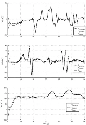
The response of the bias estimates is shown in Figure 7. Once again the asymptotic performance of the filters is similar after an initial transient. From this figure it is clear that the passive filter displays slightly less noise in the bias estimates than for the direct filter (note the different scales in the y-axis). Figures 8 and 9 relate to the second experiment. The experimental flight of the MAV was undertaken under remote control by an operator. The experimental flight plan used was: First, the vehicle was located on the ground, initially headed toward ψ(0) = 0. After take off, the vehicle was stabilized in hovering condition, around a fixed heading which remains close the initial heading of the vehicle on the ground. Then, the operator engages a ' 90o-left turn manoeuvre, returns to the initial heading, and follows with a ' 90o-right turn
0 10 20 30 40 50 60 −50 0 50 roll φ (°) φmeasure φpassive φdirect 0 10 20 30 40 50 60 −60 −40 −20 0 20 40 60 pitch θ (°) θmeasure θpassive θdirect 0 10 20 30 40 50 60 −100 −50 0 50 100 150 200 yaw ψ (°) time (s) ψmeasure ψpassive ψdirect
Fig. 6. Euler angles from direct and passive complementary filters
0 10 20 30 40 50 60 −20 −10 0 10 best−direct (°/s) time (s) b1 b2 b3 0 10 20 30 40 50 60 −5 0 5 10 best−passive (°/s) time (s) b1 b2 b3
Fig. 7. Bias estimation from direct and passive complementary filters
manoeuvre, before returning to the initial heading and landing the vehicle. After landing, the vehicle is placed by hand at its initial pose such that final and initial attitudes are the identical. Figure 8 plots the pitch and roll angles (φ, θ) estimated directly from the accelerometer measurements against the estimated values from the explicit complementary filter. Note the large amounts of high frequency noise in the raw attitude estimates. The plots demonstrate that the filter is highly successful in reconstructing the pitch and roll estimates.
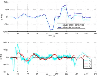
Figure 9 presents the gyros bias estimation verses the predicted yaw angle (φ) based on open loop integration of the gyroscopes. Note that the explicit complementary filter here is based solely on estimation of the gravitational direction. Consequently, the yaw angle is the indeterminate angle that is not directly stabilised in Corollary 5.2. Figure 9 demonstrates that the proposed filter has successfully identified the bias of the yaw axis gyro. The final error in yaw orientation of the microdrone after landing is less than 5 degrees over a two minute flight. Much of this error would be due to the initial transient when the bias estimate was converging. Note that the
second part of the figure indicates that the bias estimates are not constant. Although some of this effect may be numerical, it is also to be expected that the gyro bias on low cost IMU systems are highly susceptible to vibration effects and changes in temperature. Under flight conditions changing engine speeds and aerodynamic conditions can cause quite fast changes in gyro bias.
Fig. 8. Estimation results of the Pitch and roll angles.
50 60 70 80 90 100 110 120 130 140 −100 −50 0 50 100 time (s) φ (deg)
φ (yaw angle) from gyros
φ from the estimator
50 60 70 80 90 100 110 120 130 140 −0.04 −0.02 0 0.02 0.04 time (s) b (rd/s) b x by bz
Fig. 9. Gyros bias estimation and influence of the observer on yaw angle.
VII. CONCLUSION
This paper presents a general analysis of attitude observer design posed directly on the special orthogonal group. Three non-linear observers, ensuring almost global stability of the observer error, are proposed:
Direct complementary filter: A non-linear observer posed on
SO(3) that is related to previously published non-linear
observers derived using the quaternion representation of
SO(3).
Passive complementary filter: A non-linear filter equation that
takes advantage of the symmetry of SO(3) to avoid transformation of the predictive angular velocity term
into the estimator frame of reference. The resulting ob-server kinematics are considerably simplified and avoid coupling of constructed attitude error into the predictive velocity update.
Explicit complementary filter: A reformulation of the passive
complementary filter in terms of direct vectorial measure-ments, such as gravitational or magnetic field directions obtained for an IMU. This observer does not require on-line algebraic reconstruction of attitude and is ideally suited for implementation on embedded hardware plat-forms. Moreover, the filter remains well conditioned in the case where only a single vector direction is measured. The performance of the observers was demonstrated in a suite of experiments. The explicit complementary filter is now implemented as the primary attitude estimation system on several MAV vehicles world wide.
APPENDIXA
A REVIEW OFCOMPLEMENTARYFILTERING
Complementary filters provide a means to fuse multiple independent noisy measurements of the same signal that have complementary spectral characteristics [11]. For example, consider two measurements y1= x + µ1and y2= x + µ2of a
signal x where µ1 is predominantly high frequency noise and
µ2 is a predominantly low frequency disturbance. Choosing a
pair of complementary transfer functions F1(s) + F2(s) = 1
with F1(s) low pass and F2(s) high pass, the filtered estimate
is given by
ˆ
X(s) = F1(s)Y1+F2(s)Y2= X(s)+F1(s)µ1(s)+F2(s)µ2(s).
The signal X(s) is all pass in the filter output while noise components are high and low pass filtered as desired. This type of filter is also known as distorsionless filtering since the signal
x(t) is not distorted by the filter [43]. Complementary filters
are particularly well suited to fusing low bandwidth position measurements with high band width rate measurements for first order kinematic systems. Consider the linear kinematics
˙x = u. (41)
with typical measurement characteristics
yx= L(s)x + µx, yu= u + µu+ b(t) (42) where L(s) is low pass filter associated with sensor character-istics, µ represents noise in both measurements and b(t) is a deterministic perturbation that is dominated by low-frequency content. Normally the low pass filter L(s) ≈ 1 over the frequency range on which the measurement yx is of interest. The rate measurement is integratedyus to obtain an estimate of the state and the noise and bias characteristics of the integrated signal are dominantly low frequency effects. Choosing
F1(s) = C(s)
C(s) + s
F2(s) = 1 − F1(s) = s