HAL Id: halshs-00638150
https://halshs.archives-ouvertes.fr/halshs-00638150
Submitted on 4 Nov 2011
HAL is a multi-disciplinary open access archive for the deposit and dissemination of sci-entific research documents, whether they are pub-lished or not. The documents may come from
L’archive ouverte pluridisciplinaire HAL, est destinée au dépôt et à la diffusion de documents scientifiques de niveau recherche, publiés ou non, émanant des établissements d’enseignement et de
Search Intensity, Directed Search And The Wage
Distribution
Bruno Decreuse, André Zylberberg
To cite this version:
Bruno Decreuse, André Zylberberg. Search Intensity, Directed Search And The Wage Distribution. Journal of the European Economic Association, Wiley, 2011, 9 (6), pp.20-38. �halshs-00638150�
Search intensity, directed search and the wage distribution
Bruno Decreusey
University of Aix-Marseilles, GREQAM, IDEP André Zylberbergz
Université Paris I Panthéon-Sorbonne, CNRS, CES February 2010
Abstract: We propose a search equilibrium model in which homogenous …rms post wages along with a vacancy to attract job-seekers, while homogenous unemployed workers invest in costly job-seeking. The key innovation relies on the organization of the search market and the search behavior of the job-seekers. The search market is continuously segmented by wage level, individuals can spread their search investment over the di¤erent sub-markets, and search intensity has marginal decreasing returns on each sub-market. We show that there exists a non-degenerate equilibrium wage distribution. The density of this wage distribution is increasing at low wages, and decreasing at high wages. Under additional restrictions, it is hump-shaped, and it can be right-tailed. Our results are illustrated by an example originating a Beta wage distribution.
Keywords: Search e¤ort; Segmented markets; Equilibrium wage dispersion J.E.L. classi…cation: D83; J31; J41; J64
1
Introduction
This paper is a theoretical contribution to the literature on frictional wage dispersion. The size of residual wage dispersion in Mincerian wage regressions has motivated a major interest in un-derstanding of wage distribution for homogenous labor. Controlling for individual characteristics typically leaves unexplained the two thirds of the variance of the (log of the) wage distribution (Katz and Autor, 1999). Modern theories of wage dispersion provide search-theoretic micro-foundations for residual wage disparity. However, early search models have failed to generate empirically plausible wage distributions. In particular, they do not predict increasing density at low wages and decreasing density at high wages. They also fail to predict the single-peakedness This is the revised (and shorter) version of a paper that circulated under the title "Job search with ubiquity and the wage distribution". We thank Pierre Cahuc, Olivier Charlot, Pieter Gautier, Fabien Postel-Vinay, Etienne Wasmer, participants in University of Aix-Marseilles and University of Toulouse I seminars, and two referees and an editor of this review for their constructive comments.
yGREQAM, 2 rue de la charité, 13236 Marseille cedex 02, France. E-mail: [email protected]
zCES-EUREQua, Maison des Sciences Economiques, 106-112 boulevard de l’Hôpital, 75647 Paris cedex 13,
property. This particularity is usually pinned down by the explicit modelling of heterogeneity, but this is not the point. The challenge for this paper is to deliver the key properties of empirical wage distributions without the ad-hoc addition of heterogeneity.
Our paper introduces search intensity into the canonical directed search model. Directed search models have been examined by Hosios (1990), Montgomery (1991), Peters (1991), Moen (1997), and Burdett, Shi and Wright (2001). They have been enriched by Shi (2002) and Shimer (2005) to account for …rm and worker heterogeneity. In such models, the search market is segmented by wage, workers can choose which jobs they apply for, and the probability of getting a job is a decreasing function of the length of the job queue. Wage competition takes place at the time of wage/market choice. In equilibrium, all wage o¤ers must yield the same utility: if not, the jobs would not be prospected. This implies that there is a unique wage o¤er balancing workers’marginal cost of seeking the highest wage o¤er (a lower employment probability) and their marginal bene…t (a better wage once employed).
In our framework, the search market is segmented by wage, workers can choose their search investment on each market place, and the technology that transforms search investment into matching probability has marginal decreasing returns. These assumptions sustain the existence of a continuous wage distribution. Workers can compensate a lower reward by a smaller e¤ort, thereby raising the marginal productivity of e¤ort. This provides them incentives to spread their e¤orts over several sub-markets at a time. Firms respond to such incentives by posting jobs on a continuum of markets. The assumption of decreasing marginal returns is essential. When the e¢ ciency of e¤ort function has constant marginal returns to search, workers concentrate their search e¤ort on the market that yields the highest reward. The equilibrium wage distribution collapses to the only wage featured by standard directed search models.
The equilibrium wage distribution re‡ects the pattern of search investment and job o¤ers by wage. As the return to search …rst increases, and then decreases with wage, search investment evolves non-monotonically with the wage. We show that there is a unique maximum, corre-sponding to the only wage that would obtain if the marginal return to search investment were constant. The number of vacancies on each market tends to decrease with the wage, as paying higher wages must be compensated by lower search costs, and thus longer job queues. It also tends to increase with the number of e¤ective job-seekers, because recruitment rates depend on the ratio of vacancies to e¤ective number of job-seekers. The combination of these two e¤ects implies that the density of the wage o¤er distribution is increasing at low wages, and increasing at high wages. Those properties extend to the actual wage distribution – the one that counts. Provided the elasticity of the e¢ ciency of search e¤ort technology does not change too much with the amount of e¤ort, we show that both the wage o¤er distribution and the actual wage distribution admit a single peak.
The equilibrium wage distribution may also be consistent with another property of empirical wage distributions: they are right-tailed. We de…ne a long right tail by the requirement that the slope of the density of the distribution tends to zero as the wage becomes closer to the upper bound of the support of the distribution. We show that the density of the wage o¤er distribution is always right-tailed, while the density of the actual wage distribution may or may not be right-tailed. Those properties are illustrated by an example, in which the matching technology is Cobb-Douglas, and the e¢ ciency of search e¤ort is isoelastic. In that case, the actual wage distribution follows a Beta distribution and it is always hump-shaped.
inten-sity. Market segmentation is a frequent assumption in the search literature.1 Wage segmentation is a more abstract notion than segmentation by geographic or skill characteristics. However, con-sidering other types of segmentation would fail in the goal to explain residual wage dispersion as econometricians could use observable characteristics to explain residual wage disparities. Sim-ilarly, search intensity is a popular way to model the search activity. Although we know very little about the e¢ ciency of e¤ort technology, the idea thereby search investments have decreas-ing returns is widely accepted. However, our model is more demanddecreas-ing in that we require that there is such a technology in each market segment. The e¢ ciency of e¤ort technology can re-ceive a simple interpretation. In our model, workers are allowed to court the di¤erent jobs at various levels of aggressiveness. The degree of aggressiveness has decreasing returns on matching chances and varies with the wage o¤er as a result.
The reason why we consider a directed search model with endogenous search intensity can be inferred from the existing literature on frictional wage distributions.
On the one hand, undirected search models without a search intensity margin have a hard time explaining the salient features of empirical wage distributions. Diamond (1971) shows that all …rms pay the monopsony wage in the basic model with homogenous agents. Burdett-Mortensen (1998) –hereafter BM –add on-the-job search. Their model admits a non-degenerate distribution. However, the density is strictly increasing: all workers apply to high-wage jobs with a positive probability, which provides incentives for …rms to create many high-wage jobs. To obtain a single-peaked distribution, several papers add …rm heterogeneity, whether in the original BM model (see e.g. Van den Berg and Ridder, 1998, Mortensen, 2000), in models where employers can react to other …rms approaching their workers by making a countero¤er (Postel-Vinay and Robin, 2002a and 2002b), or in bargaining models with ex-post heterogeneity (Moscarini, 2005).
On the other hand, models with multiple applications easily feature equilibrium wage dis-persion, despite agents’ homogeneity and without on-the-job search. In papers with multiple applications, a worker can receive multiple o¤ers at the same time. Wage competition takes place at the time of choosing between di¤erent job o¤ers. In the random search model of Acemoglu and Shimer (2000), workers choose the number of o¤ers they receive. Acemoglu and Shimer show that there is equilibrium wage dispersion. The density of the wage o¤er distribution is strictly decreasing with a mass point at its upper bound. Galenianos and Kircher (2009) consider the directed search model of Albrecht, Gautier and Vroman (2006) in which …rms post wages and workers send multiple applications. Galenianos and Kircher assume that …rms commit to pay the posted wage irrespective of the number of job o¤ers received by the applicant. They obtain a strictly decreasing density of the wage distribution. We believe that we modelize a di¤erent eco-nomic phenomenon. In our framework, workers court jobs with various levels of aggressiveness and they can only receive a single o¤er at a time despite they search on a continuum of markets. Wage competition takes place at the time of attracting the job-seekers, and not once they have received multiple o¤ers. The two approaches o¤er complementary views of the search activity: courting jobs is probably as important as deciding among several job o¤ers. Interestingly, this is because search aggressiveness varies with the wage that we can obtain a single-peaked wage distribution.
1
In mismatch models, the search place is segmented by geographic location and workers are imperfectly mobile across locations (see Shimer, 2007). In models with two-sided heterogeneity, the search place is segmented by job type and workers choose the subset of sub-markets they participate in (see e.g. Moscarini, 2001, Gautier, 2002, and Decreuse, 2008).
Delacroix and Shi (2006) consider a directed search version of BM. Their model features a strictly decreasing wage o¤er distribution, while the actual wage distribution can be strictly decreasing, strictly increasing, or even hump-shaped. However, individuals with the same income target the same job. The wage distribution conditional on former income is degenerate as a result. In our model, unemployed workers prospect all market segments simultaneously and may end up with any wage of the wage o¤er distribution.
The rest of the paper is organized as follows. Section 2 introduces and solves our model. Section 3 focuses on the properties of the equilibrium wage distribution. Section 4 concludes.
2
The model
2.1 Preferences and technology
We study the steady state of a continuous time economy. There are a continuum of identical and in…nitely-lived workers, and a continuum of …rms. Each …rm is associated with only one job. The measure of workers is normalized to one, while the measure of …rms is endogenously determined through entry. Both are risk neutral and discount time at instantaneous rate r. Jobs can be either …lled or vacant, while workers can be either employed or unemployed. There is no on-the-job search. A worker/…rm pair produces ‡ow output y until (exogenous) separation at rate q. Unemployed workers enjoy unemployment income z, 0 z < y, while …rms endowed with a vacancy bear the ‡ow cost k.
We make four key assumptions.
First, the market is continuously segmented by wage. Segmentation follows the lines of the wage-posting search model developed, among others, by Moen (1997) and Acemoglu and Shimer (1999). Firms post vacancies with non-negotiable wages. Workers, knowing all the posted wages, choose the amount of e¤ort they will spend to search for a job. If they decide to search for a job o¤ering a wage w, they compete with other workers seeking the same wage. Symmetrically, if a …rm posts a vacancy associated with the wage w, it will compete to attract workers with the other …rms o¤ering the same wage. For each wage w, workers face a speci…c queue length and vacant jobs have a speci…c probability of being …lled. For Acemoglu and Shimer (1999), such a representation of the search process recognizes that the labor market is segmented by wages and that search frictions exist within each particular sub-market. Therefore, …rms advertise wages, and all …rms advertising a given wage and all workers applying for these jobs form a sub-market. By de…nition, the set of sub-markets is [0; 1).
Second, workers set their search intensity and allocate search e¤orts over the continuum of sub-markets. We denote by s : R+ ! R+ the function that maps the set of sub-markets into
the set of possible values for the search intensity. The overall search e¤ort is S =R01s (w) dw, where s(w) is the search intensity on the sub-market o¤ering w: This assumption looks like the directed search assumption when workers play mixed strategies. In Burdett et al (2001), workers can apply to several jobs at a time with positive probabilities. A worker’s opportunity cost of applying to a new wage is linear in the probability with which he applies there since he can only apply to the other wages with complementary probability. This cost turns out to be too high in the sense that the deviant …rms do not receive enough applications to make the same pro…ts as other …rms, even though workers would apply to a deviant wage with positive probability. However, our third assumption makes the model di¤erent from its predecessors.
The opportunity cost of applying to a particular wage is not linear as a result, and this allows …rms posting any wage along a distribution to make equal pro…ts. We denote by c : R+ ! R+
the cost of e¤ort function, with typical element c (S). It depends on overall search e¤ort S. We also de…ne x : R+ ! R+ the e¢ ciency of e¤ort function, with typical element x (s). The
technology x transforms search e¤ort into e¤ective units of search on each sub-market.
Assumption A1 The cost of e¤ ort function c : [0; +1) ! [0; +1) is strictly increasing, convex, twice di¤ erentiable, and satis…es c (0) = 0, and c0(+1) = +1:
The e¢ ciency of e¤ ort function x : [0; +1) ! [0; +1) is strictly increasing, strictly concave, twice di¤ erentiable, and satis…es x (0) = 0, x0(0) = +1, and x0(+1) = 0:
Job-seeking, like the search for ideas, has two components: tiredness and e¢ ciency. Tiredness depends on overall investment. This is why the marginal search cost depends on the aggregate search investment S. E¢ ciency depends on the amount of resources spent on the particular market that is prospected. The marginal productivity of search investment in terms of increased matching probability only depends on market-speci…c investment s.2 Such marginal productivity is decreasing, which re‡ects the fact that courting jobs more aggressively involves tasks of increasing di¢ culties.
Decreasing returns to search on each sub-market drive the existence of a non-degenerate equilibrium wage distribution. Intuitively, individuals are incited to spread their search invest-ment over the di¤erent sub-markets (and …rms are incited to participate in the corresponding sub-markets). With constant returns to search, that is with x0(s) = x0, agents would direct
their search investment toward the sub-market that yields the highest reward. There would be a single wage o¤er as a result, the competitive search equilibrium emphasized by the directed search literature with no on-the-job search (see Moen, 1997).
Fourth, agents meet according to a matching technology on each sub-market. If there are u unemployed persons in the economy, the overall search e¤ort on the sub-market o¤ering the wage w amounts to x(s (w))u where x(s (w)) denotes the market-speci…c mean e¢ ciency of search e¤orts. With v(w) vacancies o¤ering the wage w, the ‡ow number of matches on sub-market w during the small time period dt is equal to M [x(s (w))u; v(w)] dwdt. The properties of the matching technology are standard. It is twice continuously di¤erentiable, strictly increasing in each of its arguments, strictly concave with MV V < 0 and linearly homogenous: It satis…es the
boundary conditions M (U; 0) = M (0; V ) = 0, and lim
U !+1M (U; V ) = V !+1lim M (U; V ) = +1.
We impose more than strict concavity, as MV V < 0. As we discuss later, this condition is a
su¢ cient condition for the uniqueness of an equilibrium in the standard directed search model. Let (w) v (w) =x (s (w)) u be market-speci…c tightness and m ( ) M (1= ; 1). The ‡ow probability that a vacant job meets a job-seeker and the ‡ow probability that a job-seeker meets a vacant job per e¢ cient unit of search on the sub-market o¤ering the wage w are given by:
m [ (w)] dw M [x(s (w))u; v(w)]
v(w) dw
(w) m [ (w)] dw M [x(s (w))u; v(w)]
x(s (w))u dw;
2
Of course, search intensity may also have decreasing returns across the sub-markets. This could be captured by assuming that x x (s; S). In this paper we only focus on the novel aspects induced by the dependence vis-à-vis s.
In the sequel we will denote by ( ) m0( )=m( ) the elasticity of the function m( ) with respect to : The elasticity ( ) belongs to [0; 1]:
2.2 Equilibrium
We denote by Vu and Ve(w) the expected utility of an unemployed worker and of a worker paid
wage w. In the online Appendix, we show that workers can only receive one o¤er at a time. This allows us to write the standard value functions de…ning agents’expected gains. We have
rVu = max s(:) z c (S) + Z 1 0 x [s (w)] (w) m [ (w)] [Ve(w) Vu] dw (1) rVe(w) = w + q [Vu Ve(w)] (2)
It follows from (2) that workers do not prospect sub-markets whose wage is lower than the reservation wage R = rVu.
The asset values of a vacancy advertised at wage w, denoted v(w), and of a …lled job paying
w, denoted e(w), satisfy the arbitrage equations:
r v(w) = k + m [ (w)] [ e(w) v(w)] (3)
r e(w) = y w + q [ v(w) e(w)] (4)
An allocation is a tuple ( ; s; S; R; v; ), where R+ is the set of opened sub-markets,
i.e. the sub-markets that are prospected by the unemployed and the …rms that have posted vacancies.
De…nition 1 An equilibrium is an allocation ( ; s; S; R; v) such that
(i) Pro…t maximization
v(w) 0 for all w 2 R+; (5)
with equality i¤ w 2 . (ii) Optimal search intensity
s(w) = argmax s z c(S) + Z 1 R x(s) (w) m ( (w))w R r + q dw (6) R = z c(S) + Z 1 R x [s (w)] (w) m ( (w))w R r + q dw (7) with S =RR1s (w) dw.
Firms maximize pro…ts, and workers optimally spread their search investments over the di¤erent sub-markets. De…nition 1 shapes the set of opened sub-markets in equilibrium. Workers and …rms must have incentives to participate in those sub-markets. De…nition 1 also sets out-of-equilibrium beliefs that rules out situations in which …rms may not create jobs paying a potentially pro…table wage, conjecturing that none (or, at least, too few workers) would apply.
Proposition 1 Equilibrium characterization Under Assumption A1,
(i) In equilibrium, we have
= [R; y] (8) k m [ (w)] = y w r + q, 8w 2 [R; y] (9) c0(S) = x0[s(w)] (w) m [ (w)]w R r + q , 8w 2 [R; y] (10) R = z c(S) + Z y R x [s (w)] (w) m ( (w))w R r + q dw (11) S = Z y R s (w) dw (12)
(ii) There exists a unique equilibrium.
All wages belonging to the interval [R; y] are prospected, so that [R; y] is also the support of the equilibrium wage distribution. We explain this result in three steps.
First, several wages are o¤ered in equilibrium. Equilibrium wage dispersion relies on the fact that the e¢ ciency of e¤ort technology features marginal decreasing returns. This can be understood from equation (10) that describes the allocation of e¤orts over the sub-markets. The left-hand side of the equation corresponds to the marginal cost of e¤ort on sub-market w. The right-hand side corresponds to the marginal bene…t derived from searching on such a sub-market. The marginal bene…t is composed of two terms: the marginal productivity of e¤ort x0(:) times the expected reward from an additional unit of e¤ort in the sub-market. Workers can compensate a lower reward by a smaller e¤ort, thereby raising the marginal productivity of e¤ort. Workers are incited to spread their e¤orts over several sub-markets at a time. If the marginal productivity of search e¤ort were constant, workers would only invest on the sub-market that yields the highest reward. With x(s) = x0s, one can verify that the equations (9)
to (12) of Proposition 1 give a unique wage w and, consequently, a unique amount of search e¤ort spent on the unique sub-market posting the wage w.
Second, the support of the wage distribution is continuous. During the proof of Proposition 1, we show that if a wage a 2 (R; y) is not o¤ered in equilibrium, a deviant …rm can make positive pro…ts by creating such a job, which is impossible. Owing to the free-entry condition, such a pro…t opportunity must be exploited. Consequently, there are no holes in the equilibrium set of o¤ered wages.3
Third, the lower-bound of the wage distribution is R, while the upper-bound of the wage distribution is y. This results from the assumption that x0(0) = 1, and from the zero-pro…t condition featured by De…nition 1. When the wage w tends to y, the …rm’s hiring rate has to go to in…nity for the free-entry condition (9) to hold. This implies that worker’s job-…nding rate has to go to 0. Similarly, when the wage w tends to R, the wage di¤erential w R that governs search investment tends 0. Why does the worker apply to such wages? Equation (10) gives the answer. The marginal cost of such an application is c0(S), while the marginal bene…t
3The fact that the mass of …rms responds to a free-entry condition is not very important for the result of a
continuous distribution. What is important is the equal-pro…t condition that must hold on each sub-market. This condition is compatible with the assumption of a …xed number of jobs/…rms.
is proportional to x0(s (:)). This marginal bene…t can increase without limit as search intensity tends to 0.4
The job-…nding rate is =RRyx [s (w)] (w) m [ (w)] dw, that is the sum of the di¤erent rates of contact over the di¤erent markets that the job-seekers prospect. Unemployment is computed from the equality between ‡ows in and out of unemployment: q(1 u) = u. The unemployment rate is u = q= (q + ).
3
Equilibrium wage distributions
The purpose of this section is to analyze the shape of the wage distribution that is implied by our model. We proceed in three steps. First, we describe the equilibrium pattern of search investment by wage. Second, we focus on the equilibrium wage distribution. Third, we focus on the Cobb-Douglas example.
3.1 Market-speci…c search investment
Workers prospect a continuum of sub-markets in equilibrium. In this sub-section, we analyze the pattern of equilibrium search investment by wage.
Proposition 2 Search intensity Under Assumption A1,
(i) The e¤ ort function s : [R; y] ! [0; +1) satis…es s (R) = s (y) = 0;
(ii) The e¤ ort function is \-shaped, i.e. there exists a unique w 2 (R; y) such that s0(w)R 0 i¤ wS w .
The key …nding of Proposition 2 is the non-monotonicity of the relationship between wage and search investment. The pattern of search investment re‡ects the pattern of marginal reward to search. The wage has two con‡icting e¤ects. On the one hand, a higher wage raises the return to search at given market tightness, thereby motivating search investment. On the other hand, market tightness decreases with wage. A higher wage deteriorates search prospects, thereby reducing search investment. The overall e¤ect is captured by the term (w) ( (w)) y + [1 ( (w))] R w. This term is positive at low wages, while it is negative at higher wages. The search investment then reaches a maximum on the market where the reward is the highest. This corresponds to the wage w , which is implicitly de…ned by (w ) = 0. The wage w is the only wage o¤er that would result if the marginal return to search investment were constant. It is also the only wage that would result if workers could not choose their search intensity as in the standard directed search equilibrium (see e.g. Moen, 1997, and Burdett et al, 2001).5
4If x0(0)were bounded, the marginal bene…t from search e¤ort could not increase without limits. This would
restrict the interval of opened sub-markets. The bounds of the distribution would be the two roots wminand wmax
of c0(S) =x0(0) = (w) m [ (w)] (w R) = (r + q) with R < w
min< wmax< y. The assumption that x0(0) = 1
preserves simplicity without losing much insight from the case where x0(0)is bounded.
5Our model predicts a unique directed search equilibrium, while Moen (1997) shows that there may be multiple
equilibria. The reason is that we impose MV V < 0, while Moen only assumes strict concavity. The condition
3.2 Wage distribution
We distinguish the wage o¤er distribution from the actual wage distribution.
The wage o¤er distribution is the distribution of vacancies by wage. The number of vacancies advertised at wage w is v(w) = (w) x [s (w)] u, that is the product of market-speci…c tightness by the number of e¤ective job-seekers. The total number of vacancies is V =RRyv (w) dw. The cdf and the pdf of the wage o¤er distribution are then de…ned by
F (w) = Rw R v ( ) d V ; F 0(w) = v(w) V = (w) x [s (w)] u V (13)
Changes in the density F0 re‡ect changes in market tightness and search investment.
As workers court jobs paying di¤erent wages with di¤erent levels of aggressiveness, search intensity varies with the wage, and the actual wage distribution departs from the wage o¤er distribution. Let G(w) be the cdf of the actual wage distribution among employees. This cdf can be deduced from a standard ‡ow equilibrium reasoning. For each wage w 2 [R; y], the out‡ow from the pool of those employed who earn less than w equals the in‡ow from the pool of unemployed:
q(1 u)G(w) = u Z w
R
x [s( ] ( )m [ ( )] d (14)
Since q(1 u) = u, and remembering that v (w) = V F0(w) = x [s (w)] (w)u, it ensures that:
G(w) = V u
Z w R
F0( )m [ ( )] d (15)
Thus, one has:
G0(w) = V uF
0(w)m [ (w)] (16)
Changes in the density of the actual wage distribution are driven by changes in the density of the wage o¤er distribution and changes in market tightness.
Proposition 3 Wage distribution Under Assumption A1,
(i) The wage o¤ er distribution F0 : [R; y] ! [0; 1] is non-monotonic and satis…es F0(R) = F0(y) = 0. If lim
!0 ( ) > 0 and limw!y (w) < 1, F
00(y) = 0
(ii) The actual wage distribution G : [R; y] ! [0; 1] is non-monotonic and satis…es G0(R) = G0(y) = 0. Moreover, G (w) < F (w) for all w 2 (R; y)
The density of the wage o¤er distribution is non-monotonic. The density is zero at the bounds of the distribution. It is positive between those bounds. These properties mostly re‡ect the pattern of search investment by wage. Workers have very few incentives to prospect jobs that o¤er slightly more than the reservation wage. In turn, …rms do not o¤er many such jobs. Similarly, workers do not seek high-wage jobs very intensively as they know that …rms do not o¤er many of them. This strengthens …rms’incentives not to create many high-wage jobs.
As workers sample job o¤ers from the equilibrium wage o¤er distribution, the actual wage distribution is non-monotonic, increasing at low wages and decreasing at high wages. The actual wage distribution also looks better than the wage o¤er distribution. Job-seekers observe the wage o¤er distribution and alter the wage they will be paid by modulating their search investment on
each sub-market. This optimization process implies that the wage o¤er distribution …rst-order stochastically dominates the actual wage distribution.
Finally, the actual wage distribution can be right-tailed. However, unlike the wage o¤er distribution, the actual wage distribution is not always right-tailed.
Non-monotonicity does not guarantee that the wage distribution is single-peaked. The den-sity may feature multiple peaks as a result.
Assumption A2Let (s) = sxsx000(s)=x(s)=x(s)0(s). For all s 0, 0(s) x0(s) =x (s).
Assumption A2 limits the set of possible e¤ort functions by restricting the upward volatility vis-à-vis changes in search intensity. We provide further details below.
Proposition 4 Single-peak property Under Assumptions A1 and A2,
(i) The wage o¤ er distribution is \-shaped, i.e. there exists a unique w 2 (R; y) such that F00(w)R 0 i¤ w S w .
(ii) The actual wage distribution is \-shaped, i.e. there exists a unique w 2 (R; y) such that G00(w)R 0 i¤ w S w .
The wage distribution is single-peaked provided additional restrictions on the e¢ ciency of e¤ort function hold. The e¤ect of the wage on the density of the wage o¤er distribution is given by F00(w) F0(w) 0(w) (w) + x0[s (w)] x [s (w)]s 0(w) (17)
Changes in the density re‡ect the pattern of market tightness and search e¤ort by wage. The former e¤ect is negative, as …rms post fewer jobs when the wage increases. The latter e¤ect is non-monotonic. Its relative weight depends on the elasticity of the e¤ort function. This elasticity may vary so much that there may be several peaks. Assumption A2 restricts the set of e¤ort functions by imposing bounds on such variations. Such bounds are not very demanding. For instance, A2 is compatible with 0(s) 0, which encompasses the case of isoelastic e¢ ciency search functions with 0(s) = 0. In addition, A2 is a su¢ cient condition, which means that there are cases where A2 does not hold and, still, the wage o¤er distribution is hump-shaped.
These results are in sharp contrast with the literature discussed in the introduction, which predicts either increasing or decreasing density of the wage distribution6.
3.3 A Cobb-Douglas example
We consider explicit forms for the matching function and the e¢ ciency of e¤ort function. The following Proposition shows that the actual wage distribution is strongly linked with the Beta distribution.
6Halko, Kultti, and Virrankoski (2008) assume that two search places coexist. In the wage demand market,
unemployed contact vacancies; in the wage o¤er market, vacancies contact unemployed. The density of the wage distribution is increasing at low wages, decreasing at high wages, but U-shaped in the middle.
Proposition 5 The Cobb-Douglas example
Assume that m( ) = M0 ; M0 > 0; 2 (0; 1) and x(s) = s1+ ; > 0. Let ! =
(w R) = (y R) be the normalized wage, and let H be the cdf of the actual normalized wage distribution. Then, H is the cdf of a 1 ( + 1) + 1; + 1 distribution with
H0(!) = (1 !)
1 ( +1)
!
B 1 ( + 1) + 1; + 1 , 8! 2 [0; 1] where B is the Beta function such that
B (t1+ 1; t2+ 1) =
Z 1 0
(1 )t1 t2d
The Cobb-Douglas example displays several features. First, we can …nd a normalization of the wage such that the actual distribution of such a normalized wage follows a Beta distribution. Second, the parameters of the Beta distributions only involve the elasticity of the matching function and the elasticity of e¤ort function. Third, the wage distribution is single-peaked. Fourth, we can highlight the parameter circumstances under which the actual wage distribution has a ‡at right tail. Indeed, G"(y) = 0 if > (2 1) = (1 ) and G"(y) = 1 if < (2 1) = (1 ). Therefore, the wage distribution is right-tailed when the parameters of the matching function and the search function satisfy > (2 1) = (1 ). This restriction always holds when the elasticity = 1=2. Similarly, we can show that G00(R) = 0 if > 1 and
G00(R) = 1 if < 1. Therefore, the Cobb-Douglas case is consistent with an actual wage distribution characterized by a single peak, a ‡at right tail, and no left tail. This is so when (2 1) = (1 ) < < 1.
Computing the actual wage distribution requires to set all the parameters of the model. Table 1 gives the parameter values. We have the French economy in mind, where the unemployment rate u is close to 10% over the past two decades, the job loss rate q is 10% and the mean unemployment duration 1= is one year. Output is normalized to one, and unemployment income (plus value of non-labor time) accounts for 40% of output per worker. The cost of e¤ort is c (S) = c0s , 1. We choose = 2, so that the cost of e¤ort is strictly convex. The other
parameters have been set to simple values.
r q c0 M0 k y z
:05 :10 1:0 2:0 3:0 :25 1 :4 :5 1:0
Table 1: Parameter values of the baseline simulation
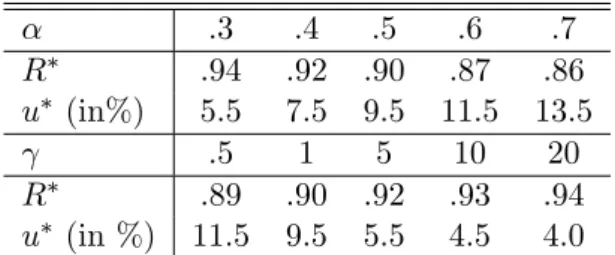
In the baseline simulation where = :5 and = 1:0, the reservation wage is R = :9 and the unemployment rate is u = 9:5%. Table 2 presents the e¤ects of changes in and on the equilibrium reservation wage and the equilibrium unemployment rate. In each case, we consider 5 di¤erent values of the parameter. When we increase the elasticity of the matching technology, the reservation wage goes down from .94 to .86, while the unemployment rate goes up from 5.5% to 13.5%. When we raise the elasticity = (1 + ) of the e¢ ciency of e¤ort technology, the reservation wage goes up from .89 to .94, while the unemployment rate goes down from 11.5% to 4.0%.
.3 .4 .5 .6 .7 R .94 .92 .90 .87 .86 u (in%) 5.5 7.5 9.5 11.5 13.5 .5 1 5 10 20 R .89 .90 .92 .93 .94 u (in %) 11.5 9.5 5.5 4.5 4.0
Table 2: Impacts of and on equilibrium reservation wage and unemployment rate.
The parameter values are given by Table 1.
Figures 1 and 2 depict the equilibrium wage distributions. Qualitatively, those distributions feature the properties described by Proposition 5. Indeed, parameters and govern the shape of the wage distribution. Figures 1 and 2 allow us to see the impacts of and on the equilibrium reservation wage. As increases, the wage distribution becomes less concentrated. Moreover, the long right tail progressively disappears. As increases, the wage distribution becomes more concentrated. When tends to in…nity, the e¢ ciency of e¤ort function has constant marginal returns. As a result, workers concentrate their search investment in the sub-market where the return is the highest. The actual wage distribution collapses to the Hosios wage w , the only wage o¤er featured by the standard directed search model.
4
Conclusion
This paper examines the choice of search intensity in the standard directed search model with homogenous agents. We make two assumptions: the search place is segmented by wage, and search investment has decreasing returns in each market segment. While setting search e¤ort in each market, workers can compensate a lower marginal return to search by a lower search investment that raises the marginal productivity of e¤ort. The model features a non-degenerate equilibrium wage distribution as a result. This equilibrium wage distribution is non-monotonic. With additional restrictions, it is also hump-shaped and right-tailed.
Unlike geographic or skill segmentation, wage segmentation is an abstract notion and the market segments can hardly be identi…able. Similarly, the shape of the search technology is exogenous and does not derive from elementary principles. However, the predicted wage dis-tribution has appealing empirical properties. The model could be enriched so as to account for on-the-job search and worker/…rm heterogeneity. In turn, the enriched model could be structurally estimated. Such a structural estimation could help revisit the respective roles of heterogeneity and frictional dispersion in the wage distribution.
The estimates could be used so as to evaluate the impacts of policy experiments like changes in payroll tax rates or in unemployment bene…ts. Compared to alternative models of the search market, our model makes a key prediction: owing to decreasing returns to search in each market segment, labor market policies have heterogenous e¤ects across market segments. Such policies should not only a¤ect employment and the mean wage, they should also a¤ect the whole wage distribution.
0.850 0.9 0.95 1 5 10 15 20 25 30 35 40 45 w age w a ge de ns ity α = .3 α = .4 α = .5 α = .6 α = .7
Figure 1: Equilibrium wage distribution and changes in the elasticity of the matching technology. Parameter goes from .3 to .7, while the other parameters are given by Table 1.
0.850 0.9 0.95 1 10 20 30 40 50 60 70 80 w age w a ge de ns ity γ = .5 γ = 1 γ = 5 γ = 10 γ = 20
Figure 2: Equilibrium wage distribution and changes in the elasticity of the e¢ ciency of e¤ort technology. Parameter goes from .5 to 20, while the other parameters are given by Table 1.
APPENDIX
A
Proof of Proposition 1
Part (i). Equations (9) to (12) directly result from De…nition 1. It remains to show that = [R; y]. First, sub-markets paying more than y involve v(w) < 0, and they must be closed.
Second, …rms cannot o¤er wages lower than R. Those jobs would not be prospected by the unemployed, implying that (w) = 1. Consequently, v(w) < 0. Third, suppose that there is
some wage a 2 (R; y) that is not o¤ered in equilibrium, and consider a particular employer who o¤ers wage b 6= a in equilibrium. This employer obtains r v(b) = k(r+q)+m[ (b)](y b)r+q+m[ (b)] = 0 by
equilibrium de…nition. The employer may think about o¤ering wage a. However, if this wage is not o¤ered in equilibrium, this must be so because the job-seekers do not invest in this market, i.e. s (a) = 0. This is compatible with equation (9) provided that (a) = 0. In such a case, the matching probability is one in any time interval for the …rm. Ex-ante pro…t is then worth r v(a) = y a > 0. The deviant …rm can make positive pro…ts, which is impossible. Wages R
and y belong to the equilibrium support by continuity.
Part (ii). Using the properties of the matching function, equation (9) de…nes a unique speci…c market tightness function (w). Then, equation (10) can be solved in s as a function of w; S and R. Let e (w; R; S) be this unique solution. From Assumption A1 and the implicit function theorem, the partial derivatives of e (w; R; S) are such that:
eS = c"(S) c0(S) x0(e) x"(e) 0; eR= 1 w R x0(e) x"(e) < 0 (18)
Now, substitute e (w; R; S) for s(w) in equation (11), and consider the function S1(R) such that
R = z c(S1) + Z y R x [e (w; R; S1)] (w) m [ (w)] w R r + q dw (19)
The derivative of the function S1(R) reads:
S10(R) = Ry ReRx0[e (w; R; S1)] (w) m [ (w)] w R r+qdw 1 = (r + q) c0(S1) Ry ReSx0[e (w; R; S1)] (w) m [ (w)] w R r+qdw = Ry ReRdw 1 RRyeSdw 1 + = (r + q) c0(S1) 1 Ry ReSdw
Hence, equation (19) implicitly de…nes S1(R) with
S10 (R) < Ry
ReRdw
1 RRyeSdw
< 0 (20)
For R = y, one has c(S1(y)) = z y < 0; which means that the function S1(R) crosses the
horizontal axis before R = y: For R = z; the value of S1(z) is given by:
c [S1(z)] = Z y z x [e (w; R; S1)] (w) m [ (w)] w R r + q dw = c 0[S 1(z)] Z y z x [e (w; z; S1(z))] x0[e (w; z; S1(z))]dw (21)
Moreover, when e (w; R; S) is substituted for s(w) in equation (12), we obtain another equa-tion de…ning a unique S as a funcequa-tion of R. We call this funcequa-tion S2(R). Di¤erentiating this
latter equation with respect to R gives: 1 Z y R eSdw dS dR = e(R; R; S) + Z y R eRdw
The properties of the matching function and equation (10) imply that e(R; R; S) = 0. Conse-quently S20 (R) = Ry ReRdw 1 RRyeSdw < 0 (22)
So far, we have shown that S0
1(R) < S20(R) < 0. In addition, S2(y) = 0. Lastly, S2(z) is given
by:
S2(z) =
Z y z
e [w; z; S2(z)] dw
Assumption A1 implies that x (e) =x0(e) > e and c(s)=c0(s) s, therefore (21) gives
S1(z) c [S1(z)] c0[S1(z)] > Z y z e [w; z; S1(z)] dw;
which proves that S1(z) > S2(z). The properties of functions S1(R) and S2(R) entail that they
cross once at a point such that R 2 (z; y). Thus, the equilibrium values of R and S are unique. It follows that the equilibrium functions (w) and s (w) given respectively by (9) and (10) are also unique.
B
Proof of Proposition 2
Part (i). Relation (9) and the properties of the matching technology imply that (y) = 0. Therefore, relation (10) and Assumption A1 imply that s(y) = 0. Furthermore, (9) shows that
(R) is …nite, and (10) and Assumption A1 then entail that s(R) = 0.
Part (ii). Let (w) [ (w)] y + [1 [ (w)]] R w. Since s is continuous and s (w) > 0 for all w 2 (R; y), the function s is non-monotonic. Di¤erentiating the logarithm of both sides of equation (10) with respect to w, we get:
x00[s(w)] x0[s(w)]s0(w) = 0(w) (w) [1 ( (w))] + 1 w R (23)
The equilibrium pattern of tightness by wage is given by equation (9). Di¤erentiating the latter equation with respect to w gives:
( (w))
0(w)
(w) = 1
y w (24)
Then, eliminating 0(w)= (w) between (23) and (24) one obtains:
s0(w) x
0[s(w)]
x00[s(w)]
(w)
Taking the derivative of function and using (24) gives: 0 (w) = 0[ (w)] [ (w)] (w) y R y w 1 (26)
The properties of the matching technology imply that [ m ( )]0 = MV(1; ) > 0 and [ m ( )] " =
MV V(1; ) < 0. As [ m( )]0 = m( ) [1 ( )], we have
[ m( )]"= m ( ) ( )(1 ( )) 0( ) (27)
It follows that:
0( ) > ( )(1 ( )) (28)
Relations (26) and (28) imply that
0(w) < 1 [ (w)]
y w (y R) 1 =
(w)
y w (29)
Therefore, 0(w) < 0 whenever (w) 0. Consequently, the equation (w) = 0 has a unique root w .
C
Proof of Proposition 3
Part (i). Let (w) = [s (w)] (w) + R w, where is de…ned during the proof of Proposition 2 and (s) = (s) = sxsx000(s)=x(s)(s)=x0(s). According to proposition 2, one has s (R) = s (y) = 0. Remembering that (y) = 0 and that (R) is …nite, relation (13) arrives at F0(R) = F0(y) = 0. Non-monotonicity results from the facts that F0 is continuous and F0(w) > 0 for all w 2 (R; y).
Using (17), (24) and (25), we have: F00(w)
F0(w) =
(w)
( (w)) (y w)(w R) (30)
Equation (30) shows that: F "(y) = lim w!y 1 ( (w)) F0(w) y wf[ ( (w)) 1] (w) 1g
Using (9) and (13), one arrives at: F "(y) = u
V k(r + q)w!ylim
(w) m ( (w)) x (s (w))
( (w)) f[ ( (w)) 1] (w) 1g
The result follows from the facts that (w) m ( (w)) and x [s (w)] tend to zero when w ! y. Part (ii). As G0(w) = V F0(w)m [ (w)] = u, part (i) of Proposition 3 implies that G0(R) = G0(y) = 0. Non-monotonicity follows from the fact that G0(w) > 0 for all w 2 (R; y) and the
continuity of G0. As m [ (w)] = k(r + q)= (y w) –see (9) –, relation (16) becomes:
G0(w) = V u
k(r + q)
y w F
Let w0 denote the unique wage such that Vuk(r+q)y w0 = 1. Suppose …rst that w0 R. One has
G0(w) < F0(w) for w < w0 and G0(w) > F0(w) for w > w0: Therefore, when w < w0 one has:
G(w) = Z w R G0( )d < Z w R F0( )d = F (w)
While, when w > w0, one has:
1 G(w) = Z y w G0( )d > Z y w F0( )d = 1 F (w) (31)
Hence, G(w) < F (w) when w0 R. Now, assume that w0 < R. Then, G0(w) > F0(w) for all
w R, and (31) holds for all w R: Consequently, G(w) < F (w) when w0 < R.
References
[1] Acemoglu, D., Shimer, R., 1999. E¢ cient unemployment insurance. Journal of Political Economy 107, 893-928
[2] Acemoglu, D., Shimer, R., 2000. Wage and technology dispersion. Review of Economic Studies 67, 587-607
[3] Albrecht, J., Gautier, P., Vroman, S., 2006. Equilibrium directed search with multiple applications. Review of Economic Studies 73, 869-891
[4] Burdett, K., Mortensen, D.T., 1998. Wage di¤erentials, employer size, and unemployment. International Economic Review 39, 257-273
[5] Burdett, K., Shi, S., Wright, R., 2001. Pricing and matching with frictions. Journal of Political Economy 109, 1060-1085
[6] Decreuse, B., 2008. Choosy search and the mismatch of talents. International Economic Review 49, 1067-1089
[7] Delacroix, A., Shi, S., 2006. Directed search on the job and the wage ladder. International Economic Review 47, 651-699
[8] Diamond, P., 1971. A model of price adjustment. Journal of Economic Theory 3, 156-168 [9] Galenianos, M., Kircher, P., 2009. Directed search with multiple job applications. Journal
of Economic Theory 144, 445-471
[10] Gautier, P., 2002. Unemployment and search externalities in a model of heterogeneous jobs and workers. Economica 273, 21-40
[11] Halko, M.-H., Kultti, K., Virrankoski, J., 2008. Search direction and wage dispersion. In-ternational Economic Review 49, 111-134
[12] Hosios, A., 1990. On the e¢ ciency of matching and related models of search and unemploy-ment. Review of Economic Studies 57, 279-298
[13] Katz, L., Autor, D., 1999. Changes in the wage structure and earnings inequality. In Hand-book of Labor Economics, vol. 3, Amsterdam: Elsevier
[14] Moen, E., 1997. Competitive search equilibrium. Journal of Political Economy 105, 385-411 [15] Montgomery, J., 1991. Equilibrium wage dispersion and interindustry wage di¤erentials.
Quarterly Journal of Economics 106, 163-179
[16] Mortensen, D.T., 2000. Equilibrium unemployment with wage-posting: Burdett-Mortensen meet Pissarides. In H. Bunzel, B.J. Christiansen, P. Jensen, N.M. Kiefer and D.T. Mortensen, eds., Panel data and structural labor market models, Amsterdam: Elsevier [17] Moscarini, G., 2001. Excess worker reallocation. Review of Economic Studies 68, 593-612 [18] Moscarini, G., 2005. Job matching and the wage distribution. Econometrica 73, 481-516 [19] Peters, M., 1991. Ex ante price o¤ers in matching games: Non-steady states. Econometrica
59, 1425-1454
[20] Postel-Vinay, F., Robin, J.-M., 2002a. The distribution of earnings in an equilibrium search model with state-dependent o¤ers and countero¤ers. International Economic Review 43, 989-1016
[21] Postel-Vinay, F., Robin, J.-M., 2002b. Wage dispersion with worker and employer hetero-geneity. Econometrica 70, 2295-2350
[22] Shi, S., 2002. A directed search model of inequality with heterogeneous skills and skill-biased technology. Review of Economic Studies 69, 467-491
[23] Shimer, R., 2005. The assignment of workers to jobs in an economy with coordination frictions. Journal of Political Economy 113, 996-1025
[24] Shimer, R., 2007. Mismatch. American Economic Review 97, 1074-1101
[25] Van den Berg, G., Ridder, G., 1998. An empirical equilibrium search model of the labor market. Econometrica 66, 1183-1221