Decoding MT Motion Response For Optical Flow Estimation : An Experimental Evaluation

HAL Id: hal-01215526

https://hal.inria.fr/hal-01215526

Submitted on 19 Oct 2015

HAL is a multi-disciplinary open access

archive for the deposit and dissemination of

sci-entific research documents, whether they are

pub-lished or not. The documents may come from

teaching and research institutions in France or

abroad, or from public or private research centers.

L’archive ouverte pluridisciplinaire HAL, est

destinée au dépôt et à la diffusion de documents

scientifiques de niveau recherche, publiés ou non,

émanant des établissements d’enseignement et de

recherche français ou étrangers, des laboratoires

publics ou privés.

Decoding MT Motion Response For Optical Flow

Estimation : An Experimental Evaluation

Manuela Chessa, N. V. Kartheek Medathati, Guillaume Masson, Fabio Solari,

Pierre Kornprobst

To cite this version:

Manuela Chessa, N. V. Kartheek Medathati, Guillaume Masson, Fabio Solari, Pierre Kornprobst.

Decoding MT Motion Response For Optical Flow Estimation : An Experimental Evaluation. 23rd

European Signal Processing Conference (EUSIPCO), Aug 2015, Nice, France. �hal-01215526�

DECODING MT MOTION RESPONSE FOR OPTICAL FLOW ESTIMATION: AN

EXPERIMENTAL EVALUATION

Manuela Chessa

, N. V. Kartheek Medathati

, Guillaume S. Masson

, Fabio Solari

, Pierre Kornprobst

_{University of Genova, DIBRIS, Italy}

†

_{INRIA, Neuromathcomp team, Sophia Antipolis, France}

_{Institut des Neurosciences de la Timone, CNRS, Marseille, France}

ABSTRACT

Motion processing in primates is an intensely studied prob-lem in visual neurosciences and after more than two decades of research, representation of motion in terms of motion en-ergies computed by V1-MT feedforward interactions remains a strong hypothesis. Thus, decoding the motion energies is of natural interest for developing biologically inspired computer vision algorithms for dense optical flow estimation. Here, we address this problem by evaluating four strategies for motion decoding: intersection of constraints, linear decoding through learned weights on MT responses, maximum likelihood and regression with neural network using multi scale-features. We characterize the performances and the current limitations of the different strategies, in terms of recovering dense flow es-timation using Middlebury benchmark dataset widely used in computer vision, and we highlight key aspects for future de-velopments.

Index Terms— Optical flow, spatio-temporal filters,

mo-tion energy, populamo-tion code, V1, MT, Middlebury dataset, 1. INTRODUCTION

Visual motion estimation is a widely studied problem in both computer vision and visual neuroscience. How do primates estimate motion has been a question of intense focus in vi-sual neuroscience yet only partly understood owing both to underlying complexity and to the experimental stimuli that has been used (see [1] for a review). The limitations of the experimental and modeling studies in motion estimation so far have been well explained by Nishimoto et al. [2], in terms of partial coverage in spatio-temporal frequency domain, e.g., only direction of motion [3, 4] or two-dimensional slice [5, 6]. Though in [2] the authors show that the widely accepted feed-forward spatio-temporal filtering model is a good fit for ex-plaining neural responses to naturalistic videos, the model has not been tested in terms of recovering the dense velocity vec-tor field, called optical flow, which has been extensively stud-ied in computer vision due to its broad application potential. (see [7] for a review)

Both authors M. C. and N.V.K. M. should be considered as first author.

It is not clear how these spatio-temporal filter based mod-els deal with several naturalistic scenarios such as motion boundaries, and occlusions. It is also not clear how these methods could produce a spatially accurate estimation in term of recovering dense optical flow as filter-based models tend to smooth the images. Modern computer vision datasets with ground truth, such as Middlebury dataset [8], give us an op-portunity to study these aspects also with respect to the prob-lem of decoding. The goal of this paper is to evaluate four de-coding strategies to estimate optical flow from motion tuned population response.

This paper is organised as follows. In Sect. 2, we present the basis of our approach, which is a feedforward model of V1 and MT cortical areas: We start from the model [9] in which we revisited the seminal work by Heeger and Simon-celli [10, 11] (see Fig. 1). In Sect. 3, we propose three de-coding strategies to estimate optical flow based on MT popu-lation response and a fourth one based on V1 popupopu-lation re-sponse. These four strategies are then evaluated and discussed in Sect. 4 using classical sequences from the literature.

EV 1 _EM T v1 + v1 + v2 S0 S2 S1 cv2 cv1 cv0 x,y ⇤ x,y ⇤ x,y ⇤ t ⇤ t ⇤ t ⇤ Warp Warp v2 EV 1 _EM T EV 1 EM T Figure 2

Fig. 1. Illustration of the FFV1MT approach [9] based on a feedforward model of V1 and MT cortical layers and a coarse to fine implementation. At each scale, decoded velocities at a coarser scale are used to warp V1 motion energies at the finer scale (shown in red). Code available on ModelDB: http://senselab.med.yale.edu/modeldb.

2. V1-MT MODEL FOR MOTION PROCESSING This section describes how V1 and MT responses are esti-mated at a given scale and we refer the reader to [9] for more details about the coarse to fine approach (see Fig. 1).

2.1. Area V1: Motion Energy

Simple cells are characterized by the preferred spatial ori-entation θ of their contrast sensitivity in the spatial domain and their preferred velocity vc in the direction orthogonal to their contrast orientation often referred to as component speed. The receptive fields of the V1 simple cells are classi-cally modeled using band-pass filters in the spatio-temporal domain. In order to achieve low computational complexity, the spatio-temporal filters are decomposed into separable fil-ters in space and time. Spatial component of the filter is de-scribed by Gabor filters h and temporal component by an ex-ponential decay function k. We define the following complex filters: h(p; θ, fs) =Be ( −(x2+y2) 2σ2 ) ej2π(fscos(θ)x+fssin(θ)y)_, k(t; ft) =e(− t τ)ej2π(ftt)_,

where σ and τ are the spatial and temporal scales respectively, which are related to the spatial and temporal frequencies fs

and ftand to the bandwidth of the filter. Denoting the real and

imaginary components of the complex filters h and k as he, ke

and ho, korespectively, and a preferred velocity (speed

mag-nitude) vc _{= f}

t/fs, we introduce the odd and even

spatio-temporal filters defined as follows,

go(p, t; θ, vc, σ) =ho(p; θ, fs)ke(t; ft) + he(p; θ, fs)ko(t; ft),

ge(p, t; θ, vc, σ) =he(p; θ, fs)ke(t; ft)− ho(p; θ, fs)ko(t; ft).

These odd and even symmetric and tilted (in space-time do-main) filters characterize V1 simple cells. Using these ex-pressions, we define the response of simple cells, either odd or even, with a preferred direction of contrast sensitivity θ in the spatial domain, with a preferred velocity vc _{and with a}

spatial scale σ by

Ro/e(p, t; θ, vc, σ) = go/e(p, t; θ, vc, σ) (p,t)

∗ I(p, t), (1)

where I(p, t) is a gray-scale sequence, defined at positions

p = (x, y) and time t > 0. The complex cells are described

as a combination of the quadrature pair of simple cells (1) by using the motion energy formulation,

E(p, t; θ, vc, σ) = Ro(p, t; θ, vc, σ)2+ Re(p, t; θ, vc, σ)2,

followed by a normalization: assuming that we consider a finite set of orientations θ = θ1. . . θN, the final V1 response

is given by EV 1(p, t; θ, vc, σ) = E(p, t; θ, v c_{, σ)} ∑N i=1E(p, t; θi, vc, σ) + ε , (2)

where 0 < ε ≪ 1 is a small constant to avoid divisions by zero in regions with no energies, which happens when no spatio-temporal texture is present.

2.2. Area MT: Pattern Cells Response

MT neurons exhibit velocity tuning irrespective of the local structure orientation. This is believed to be achieved by pool-ing afferent V1 responses in both spatial and orientation do-mains followed by a non-linearity [4, 11]. The response of a MT pattern cell tuned to the speed vcand to direction of speed

d can be expressed by EM T(p, t; d, vc, σ) = F (_N ∑ i=1 wd(θi)P(EV 1)(p, t; θi, vc, σ) ) ,

where wdrepresents the MT linear weights that give origin to

the MT tuning. It can be defined by a cosine function shifted over various orientations [4, 12], i.e.,

wd(θ) = cos(d− θ) d ∈ [0, 2π[.

Then,P(EV 1_{) corresponds to the spatial pooling and is}

de-fined by P(EV 1_{)(p, t; θ} i, vc, σ) = 1 A ∑ p′ fα(∥p−p′∥)EV 1(p, t; θi, vc, σ), (3) where fα(s) = exp(s2/2α2),∥.∥ is the L2-norm, α is a

con-stant, A is a normalization term (here equal to 2πα2_{) and}

F (s) = exp(s) is a static nonlinearity chosen as an

expo-nential function [4]. The pooling defined by (3) is a spatial Gaussian pooling.

Figure 2 shows examples of MT responses at (a) single cell and (b) population levels. In this paper, the velocity space was sampled by considering MT neurons that span over the 2-D velocity space with a preferred set of Q = 19 tuning speed directions d1..dQin [0, 2π[ and M = 7 tuning speeds v1c..vMc

in the range±1 pixel/frame.

3. DECODING OF THE VELOCITY REPRESENTATION OF AREA MT

In order to engineer an algorithm capable of recovering dense optical flow estimates v(p, t) = (vx, vy)(p, t), we need to

address the problem of decoding the population responses of tuned MT neurons. Indeed, a unique velocity vector cannot be recovered from the activity of a single velocity tuned MT neuron as multiple scenarios could evoke the same activity. However, a unique vector can be recovered from the popula-tion activity of MT cells tuned to different mopopula-tion direcpopula-tions. Four decoding strategies are proposed and evaluated. We first propose three decoding methods for computing velocity from the MT response at each scale [9] (see Fig. 1)

(a) (b)

Fig. 2. MT response. (a) Example of an MT direction tun-ing curve for a cell tuned at d = π/5 respondtun-ing to movtun-ing random dot stimuli that span all the speed directions. (b) Ex-ample of MT population response at a given image point p, for a random dot sequence that moves at vx= 0.3 and vy = 0.3

pixel/frame. The MT population response shows a peak for the direction and the speed present in the input stimulus. The range of the responses is between 0.7 and 1.3.

weights (LW), and maximum likelihood (ML). Note that these

decoding methods will impact the quality of the optical flow extracted at each scale and used for the warping. Then we propose a fourth strategy, called regression with neural

net-work (RegNN), which learns to estimate optical flow directly

from the V1 responses at every scales.

3.1. Intersection of Constraints Decoding (IOC)

The MT response is obtained through a static nonlinearity scribed by an exponential function, thus we can linearly de-code the population activities [13]. Since the distributed rep-resentation of velocity is described as a function of two pa-rameters (speed vc _{and direction d), first we linearly decode}

the speed (velocity magnitude) for each speed direction, then we apply the IOC [1] to compute the speed direction. The speed along direction d can be expressed as:

vd(p, t; d, σ) =

M

∑

i=1

vc_iEM T(p, t; d, v_ic, σ). (4)

Then the IOC solution is defined by solving the minimization problem v = argmin w {G(w)} (5) where G(w) = Q ∑ i=1 (vdi− w · (cos d i, sin di)T)2

where (·)T _{indicates the transpose operation. Solving (5)}

gives: vx=_Q2 ∑Q i=1v d_{(p, t; d} i, σ) cos di, vy= _Q2 ∑Q i=1v d_{(p, t; d} i, σ) sin di.

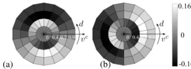
3.2. Linear Decoding Through Learned Weights (LW) The MT response can be decoded by learning the two-dimensional matrix of weights W so that v = EM T_W.

(a) (b)

Fig. 3. Two-dimensional matrices of weights learned using sequences of random dots and used to decode (a) vxand (b)

vy. In these plots, we represent only half of the matrixW for

vc_{= [0; 0.4; 0.7; 0.9].}

To learn the weights, we used a dataset of 8× 7 random dot sequences with known optical flow vgt (8 directions and 7

speeds), which cover the spatio-temporal filters’ range, and we estimatedW by minimizing the cost function L:

L(W) = ||RW − vgt||2+ λ||W||2, (6)

where R is a matrix whose rows contain the MT popula-tion responses (for the whole training set),W is the vector of weights, vgtcontains the ground truth speeds,|| · || is the

L2-norm and we chose λ = 0.05. It is worth to note that such

procedure has been carried out at a single spatial scale. Since we use random dots, we have considered the average MT re-sponse. Figure 3 shows the learned two-dimension matrix of weights.

3.3. Maximum Likelihood Decoding (ML)

The MT response can be decoded with a Maximum Like-lihood technique [14]. In this paper, the ML estimate is performed through a curve fitting, or template matching, method. In particular, we decode the MT activities by finding the Gaussian function that best match the population re-sponse. The position of the peak of the Gaussian corresponds to the ML estimate.

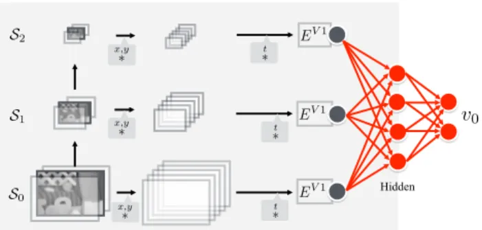
3.4. Decoding by Regression with Neural Network (RegNN) For the regression using neural network, spatio-temporal en-ergies representative of the V1 complex cell responses are computed across various scales and are concatenated to form an input vector of dimension 504 (6 scales× 12 orientations

× 7 velocities). The feature computation stage is illustrated

in Fig. 4. It is worth to note that in this decoding strategy we do not use the coarse to fine approach. We use a feedforward network comprising of a hidden sigmoidal layer and a linear output layer with 400 neurons in the hidden layer and 2 neu-rons in the output layer, computing velocity along x and y axis. The hidden layer can be interpreted as MT cells tuned to different velocities. For training the network, subsampled features by a factor of 30 from Middlebury sequences are used and the network is trained for 500 epochs using back propaga-tion algorithm till the RMSE of the network over the training

EV 1 S0 S2 S1 x,y ⇤ x,y ⇤ x,y ⇤ t ⇤ t ⇤ t ⇤ EV 1 EV 1 Figure 2 v0 Hidden

Fig. 4. Scale space for regression based learning (see Sect. 3.4).

samples has reached 0.3. Note that we only have a single network or a regressor and it is applied to all pixels. For train-ing and simulattrain-ing the experiment PyBrain package has been used.

4. EXPERIMENTAL EVALUATION AND DISCUSSION

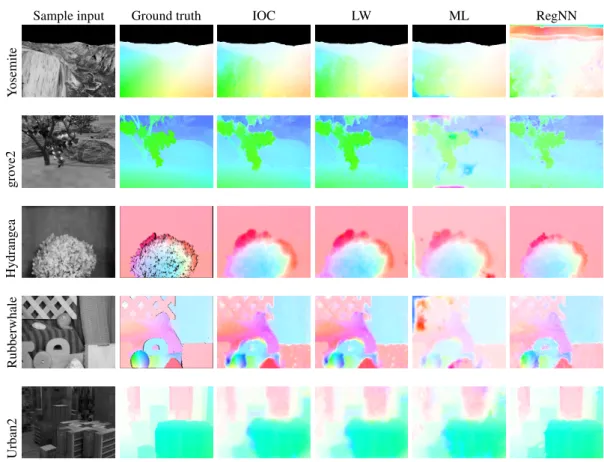
Table 1 shows the average angular errors (AAE) and the end-point errors (EPE) with the corresponding standard de-viations, by considering the Middlebury training set and the Yosemite sequence. Results for the four decoding strategies (IOC, LW, ML and RegNN) are reported. Some sample opti-cal flows for the four decoding methods are reported in Fig. 5. Results show that the IOC approach gives estimates similar to the ones obtained by considering LW. The ML approach does not perform as well as the IOC one: this is due to the actual MT activity pattern, and to the fact that MT population responses for low speed has several peaks and it is hard to fit a Gaussian.

Observing the results obtained after decoding suggests that scale-space with warping procedure is not well suited for analysis with spatio-temporal features and produces larger errors when compared to the regression scheme where the spatio-temporal motion energies across scales are simultane-ously taken into consideration. This is in accordance with ear-lier model by Heeger, where plane fitting in spatio-temporal domain has been adapted, indicating that interscale interac-tions are critical in velocity decoding. The RegNN approach has preserved motion edges much better when compared to the warping scheme in most of the sequences, but however it fails in the Yosemite sequence, which indicates that there is some diffusion happening in regions without motion energy as could be seen in the sky region. The responses of the network need to be more smooth to better match the ground truth, however this is to be expected as this regression scheme does not have any neighborhood interactions and smoothness criterion in place.

As a whole, this paper provides a first comparative study of several motion estimation approaches by population

decod-ing. Results are promising although further invastigations are needed to reach the state-of-the-art performances. Our future work will focus on incorporating spatial pooling of motion energies and spatial interaction at MT level into the model.

Acknowledgments

The research leading to these results has received funding from the European Union’s Seventh Framework Programme (FP7/2007-2013) under grant agreement no. 318723 (MATH-EMACS), and from the PAR-FAS 2007-2013 (regione Ligu-ria) project ARIANNA.

REFERENCES

[1] D. C. Bradley and M. S. Goyal, “Velocity computation in the primate visual system,” Nature Reviews

Neuro-science, vol. 9, no. 9, pp. 686–695, 2008.

[2] S. Nishimoto and J. L. Gallant, “A three-dimensional spatiotemporal receptive field model explains responses of area MT neurons to naturalistic movies,” The Journal

of Neuroscience, vol. 31, no. 41, pp. 14551–64, 2011.

[3] C.C. Pack and R.T. Born, “Temporal dynamics of a neural solution to the aperture problem in visual area MT of macaque brain,” Nature, vol. 409, no. 6823, pp. 1040–2, 2001.

[4] N.C. Rust, V. Mante, E.P. Simoncelli, and J.A. Movshon, “How MT cells analyze the motion of vi-sual patterns,” Nature Neuroscience, vol. 9, no. 11, pp. 1421–1431, 2006.

[5] J. Perrone and A. Thiele, “Speed skills: measuring the visual speed analyzing properties of primate MT neu-rons,” Nature Neuroscience, vol. 4, no. 5, pp. 526–32, 2001.

[6] N. Priebe, C. Cassanello, and S. Lisberger, “The neu-ral representation of speed in macaque area MT/V5,”

Journal of Neuroscience, vol. 23, no. 13, pp. 5650–61,

2003.

[7] D. Fortun, P. Bouthemy, and C. Kervrann, “Optical flow modeling and computation: a survey,” Computer Vision

and Image Understanding, vol. 134, pp. 1–21, 2015.

[8] S. Baker, D. Scharstein, J.P. Lewis, S. Roth, M. Black, and R. Szeliski, “A database and evaluation method-ology for optical flow,” International Journal of

Com-puter Vision, vol. 92, no. 1, pp. 1–31, 2011.

[9] F. Solari, M. Chessa, N.V.K. Medathati, and P. Korn-probst, “What can we expect from a V1-MT feedfor-ward architecture for optical flow estimation?,” Signal

Processing: Image Communication, 2015.

[10] D.J. Heeger, “Optical flow using spatiotemporal filters,”

International Journal of Computer Vision, vol. 1, no. 4,

IOC LW ML RegNN

Sequence AAE± STD EPE± STD AAE± STD EPE± STD AAE± STD EPE± STD AAE± STD EPE± STD

grove2 4.3± 10.3 0.3± 0.6 4.6± 9.7 0.3± 0.6 9.8± 21.1 0.8± 1.3 5.2± 8.5 0.4± 0.5 grove3 9.7± 19.0 1.1± 1.8 9.9± 18.8 1.2± 1.8 13.7± 25.7 1.5± 2.3 9.7± 15.4 1.0± 1.4 Hydrangea 6.0± 11.2 0.6± 1.0 6.3± 11.8 0.7± 1.0 8.9± 20.4 0.9± 1.4 3.2± 6.2 0.3± 0.4 RubberWhale 10.2± 17.7 0.3± 0.5 10.1± 16.7 0.3± 0.5 16.3± 26.3 0.7± 1.5 7.6± 9.0 0.3± 0.3 urban2 15.2± 10.2 0.6± 1.1 16.5± 22.8 1.5± 1.9 14.2± 20.4 1.5± 1.9 4.6± 9.7 0.3± 0.6 urban3 15.8± 35.9 1.9± 3.2 14.1± 33.3 1.7± 3.1 18.2± 39.5 1.8± 2.9 5.8± 17.5 0.8± 1.5 Yosemite 3.5± 2.9 0.2± 0.2 3.8± 3.0 0.2± 0.2 5.3± 7.2 0.3± 0.7 20.1± 14.7 0.9± 0.9 all 9.2± 15.3 0.7± 1.2 9.3± 16.6 0.8± 1.3 12.3± 22.9 1.1± 1.7 8.0± 11.6 0.6± 0.8 Table 1. Error measurements on Middlebury training set and on the Yosemite sequence.

Sample input Ground truth IOC LW ML RegNN

Y osemite gro v e2 Hydrangea Rubberwhale Urban2

Fig. 5. Sample results on a subset of Middlebury training set and on the Yosemite sequence (see Tab. 1 for the quantitative evaluation).

[11] E. P. Simoncelli and D. J. Heeger, “A model of neuronal responses in visual area MT,” Vision Research, vol. 38, no. 5, pp. 743 – 761, 1998.

[12] J. H. Maunsell and D. C. Van Essen, “Functional prop-erties of neurons in middle temporal visual area of the macaque monkey. I. Selectivity for stimulus direction, speed, and orientation,” Journal of Neurophysiology, vol. 49, no. 5, pp. 1127–1147, 1983.

[13] K. R. Rad and L. Paninski, “Information rates and op-timal decoding in large neural populations,” in NIPS, 2011, pp. 846–854.

[14] A. Pouget, K. Zhang, S. Deneve, and P. E. Latham, “Statistically efficient estimation using population cod-ing,” Neural Computation, vol. 10, no. 2, pp. 373–401, 1998.