NUMERICAL SIMULATION OF TURBULENT THERMAL MIXING IN A RECTANGULAR T-JUNCTION

85

NUMERICAL SIMULATION OF TURBULENT

THERMAL MIXING IN A RECTANGULAR

T-JUNCTION

Bessaid Bouchera Sara,

Dellil Ahmed Zineddine,

Nemdili Fadéla,

&

Azzi Abbès

1

_{Département ELM, Institut de Maintenance et de Sécurité Industrielle, Université Oran 2,}

Oran, Algeria

2

_{Laboratoire Aero Hydrodynamique Navale, (LAHN) USTO-MB, Oran, Algeria}

3

_{Université des Sciences et de la Technologie d’Oran, Mohamed Boudiaf, Faculté de Génie}

Mécanique, BP1505 El-Mnaouar, 31000, Oran, Algeria

*Address all correspondence to: Bessaid Bouchera Sara, Département ELM, Institut de Maintenance et de Sécurité Industrielle, Université Oran 2, Oran, Algeria; Tel.: +213 06 67 43 55 35; Fax: +213 41 64 81 48, E-mail: bestsara2010@hotmail.fr

Original Manuscript Submitted: 12/22/2016; Final Draft Received: 12/23/2016

This work reports three-dimensional simulation results of thermal mixing in a rectangular T-junction configuration at high Reynolds number. The validation data are provided by an experimental study done at the Department of Mechanical Engineering of Mie University, Japan. The T-junction was selected as a benchmark for thermal mixing in the ERCOFTAC Workshop held in EDF Chatou, France, 2011. Reynolds-averaged Navier-Stokes (RANS), unsteady Reynolds-averaged Navier-Stokes (URANS), and scale-adaptive simulation (SAS) were performed with CFD code using the finite-volume method. Velocity and thermal field as well as the turbulent stresses are reported and compared to experimental data in several longitudinal stations. It was found from the comparison that URANS methodology cannot reproduce the striping phenomenon, and secondly, that the SAS model fit better than the shear stress transport model with experimental data. Additional contours of averaged longitudinal velocity end thermal field as well as the flow structures developing in the channels are presented and discussed.

KEY WORDS: turbulence models, SAS-SST, URANS, T-junction, striping

1. INTRODUCTION

Thermal mixing in T-junction configurations is found in various industrial equipment, including chemical reactors, combustion chambers, piping systems in power plants, and HVAC (heating, ventilating, air-conditioning) units used for automobile air-conditioning systems (Kitada et al., 2000). The phenomenon could potentially lead to thermal fatigue failures in energy cooling systems when cyclic stresses are imposed on the piping system due to rapid temperature changes in regions where cold and hot flows are intensively mixed. Additionally, the hot and cold fluids impinge at nearly right angles, a situation lending itself to advanced CFD analysis. The fluctuating thermal field which leads to thermal fatigue can be of dramatic consequence in relation to the nuclear reactor cooling systems (Chapuliot et al., 2005). In many studies, thermal striping has been identified in light water reactors, in particular, as incidents of high-cycle fatigue at coolant mixing T-junctions (Walker et al., 2009).

Flow separation and reattachment, secondary flow, anisotropy of turbulent stresses, and heat transfer (including thermal striping) are some of the complex flow features associated with the T-junction. In order to develop effective

86

× ×

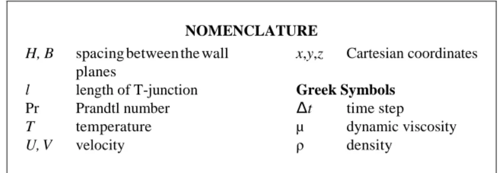
NOMENCLATURE

H, B spacing between the wall planes

l length of T-junction Pr Prandtl number

T temperature

U, V velocity

x,y,z Cartesian coordinates

Greek Symbols

∆t time step

µ dynamic viscosity

ρ density

methods to promote mixing and control thermal striping, one has to resort to advanced experimental and modeling strategies to fully understand the detailed flow and heat transfer characteristics. It is thus expected that the choice of turbulence models is a key element for successful prediction. For such applications, past experience shows that statistical time-average models need to be replaced by more sophisticated scale-resolving strategies. This paper uses the well-documented experiment done by Hirota et al. (2010) as a benchmark for CFD validation. In their project, Hirota et al. (2010) have been conducting experimental study on turbulent mixing of hot and cold airflows in a T- junction with a rectangular cross section. In their experimental data, the authors provide detailed measurements of both dynamical and thermal turbulent fields. This test case has been selected by the 15th ERCOFTAC Workshop on Refined Turbulence Modelling (WikiProjects, 2011) as a benchmark for turbulent convection mixing. In addition to steady-state and transient Reynolds-averaged Navier-Stokes (RANS) simulation with the shear stress transport (SST) turbulence model of Menter (1993), this paper presents results from the very promising new strategy of the scale-adaptive simulation model proposed by Menter and Egorov (2005).

2. T-JUNCTION TEST-CASE DESCRIPTION

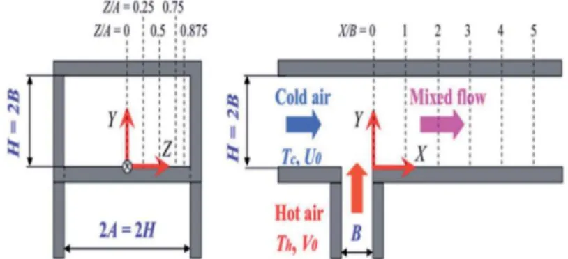
A series of detailed measurements of turbulent thermal mixing was carried out at the Department of Mechanical Engineering, Mie University, Kurimamachiya-cho, Japan, by Hirota et al. (2010). Figure 1 shows a sketch of the test channel, coordinate system, dimensions, and boundary conditions.

The flow in the main horizontal channel, which is the larger duct, is at 12◦C and the flow in the vertical branch corresponds to the hot flow at 60◦C. The two flows are maintained at the same blowing velocity of 2.7 m/s. The rectangular cross section of the main channel has a dimension of 0.12 0.06 m, while for the branch it is 0.12

0.03 m. The working fluid is air at Pr = 0.71. Experimental measurements data are provided for selected planes in both streamwise and spanwise directions, as illustrated in Fig. 2.

FIG. 1: Schematic diagram of the test channel

87

× ×

FIG. 2: Location of measurements and comparison data in Hirota et al. (2010)

3. COMPUTATIONAL DOMAIN, BOUNDARY CONDITIONS, AND COMPUTATIONAL MESHES

Three hexahedral meshes were generated for the geometry of the T-junction test case, starting with a moderate grid resolution (1.3 million) and then a refined mesh showing reasonably good near-wall refinement with about 3 million mesh nodes. As all computational domains are rectangular, the mesh quality is maintained at the best level with strictly Cartesian meshes and adequate refinement near all wall boundaries. Nominal velocity of 2.7 m/s, in accordance with experimental data in both main and branch pipes, has been specified. The given inlet length allows for a fairly well- developed turbulent velocity profile at the mixing in the T-junction. In addition, a medium turbulence intensity level of 5% is specified at the main inlet while only 2% is set for the branch. A zero averaged static pressure outlet boundary condition (BC) has been used for the outlet cross section, and nonslip BCs with automatic wall treatment are used for all walls of the domain. First, a sensitivity study on the two meshes was carried out using steady-state RANS simulation with the SST turbulence model (Menter, 1993). Profiles of mixing temperatures are compared and showed small differences in regions of large gradient; so the fine mesh is adopted and considered a mesh-independent solution. This mesh is built by 90 90 nodes in the main channel and 90 90 nodes in the branch channel. The main channel has 60 nodes from main inlet until the branch and 150 nodes from the branch until the outlet boundary, while the branch is made with 60 nodes from the branch inlet until the main channel. So, the total mesh size is nearly 3 million nodes (see Fig. 3).

The length of the computational domain is set to 4 times the width of the branch (B) from inlet to the first edge of the T-junction and 10 times from the last edge of the T-junction to the outlet boundary, while the branch is 4 times long.

FIG. 3: Grid

88

Conforming to the experimental test, the coordinate system is set with x downstream, y crossflow, and z spanwise, with the (x,y,z) = (0,0,0) origin downstream of the center of the vertical branch. Results will be provided along specified lines as shown in Fig. 2.

4. THE TURBULENCE MODELS

The first-order, two-equation model called a shear stress transport turbulence model (Menter, 1993) is used as a reference for three kinds of computations. The first one uses the steady-state SST turbulence model (RANS), the second one the unsteady RANS (URANS) formulation, also with an SST turbulence model, and then the new scale- adaptive simulation (SAS). The SST turbulence model is known to provide a good compromise by combining the k-omega model of Wilcox in the near-wall region and the high Reynolds k-ε model in the outer region. The use of the two models is realized via a blending function, which switches dynamically and smoothly from one to zero, depending on the geometrical position of the integration point. The near-wall field is resolved by use of the automatic wall functions. A detailed explanation of the model formulation and test-case validations can be found in specific literature of Menter’s group. The first computation was conducted until convergence using the steady-state RANS SST model. For the second computation, the solution obtained previously with the SST model has been used as an initialization for a transient URANS-SST simulation. The time step was set at ∆t = 0.0001 s with a second-order backward time discretization. The 10−4 maximal residual was reached with less than three loops per time step. As expected from other researchers investigating a similar T-junction but with a circular cross section, the behavior of the URANS SST solution is quickly approaching a steady-state solution in terms of velocity and temperature fields after some initial transient behavior.

This can be explained by the nature of the URANS strategy itself, which cannot provide any spectral content, even if the grid and time-step resolution would be sufficient for that purpose. This behavior is a natural outcome of the RANS averaging procedure, which eliminates all turbulence content from the velocity field. So, URANS can only work in situations of a “separation of scales.” But for this practical application and as stated before, experimental observations clearly state strong and high-frequency temperature fluctuations at pipe walls downstream of the T- junction, which can lead to high-cycle thermal fatigue, crack formation, and pipeline breaks, e.g., in pipelines in power plants. So, in that situation there is a real need to use other turbulence modeling strategies such as large eddy simulation (LES) or detached eddy simulation (DES). LES is based on the concept of filtering the flow field by means of a space filter. The specific supergrid part of the flow with its turbulent fluctuating content is directly predicted whereas the subgrid scale (SGS) part is modeled, assuming that these scales are more homogeneous and universal in behavior. This approach can give very interesting results for this test case but has the inconvenience to be very expensive, especially in terms of resolution near solid walls (Braillard et al., 2005; Hu and Kazimi, 2003). To overcome the restriction in term of computational grid sizes and consequently the running time, DES combines LES and URANS strategies and gives a very promising tool to predict industrial flows (Braillard et al., 2005; Hu and Kazimi, 2003).

Nevertheless, there is still an ambiguity in mixing two different physics in the same computation (averaged and instantaneous values). The so-called scale-adaptive simulation model was recently proposed by Menter and Egorov (2005) as a new method for the simulation of unsteady turbulent flows. A complete description of the SAS model can be found in the related publications and only a brief description is provided here. While all two-equation tur- bulence models use the same transport equation of kinetic energy as the first equation, they show a large difference in formulating the second equation. The construction of this second equation is not as straight and clear as the first one. According to Menter and Egorov (2005), Rotta’s k-kL turbulence model is well suited for term-by-term model- ing and shows some interesting features compared to other approaches. Nevertheless, the weakest part made in this model is in neglecting the second velocity derivative and maintaining the third one. The model is then suited only for homogenous turbulence and needs additional terms to be applied in the near-wall zones. Menter and Egorov (2005) suggest then to replace the problematic third velocity derivatives with the second one. The formulation proposed by Menter can operate in standard RANS mode but has the capability of resolving the turbulent spectrum in unsteady flow regions.

89

This is done by use of the von Karman length scale, LνK, which is a three-dimensional generalization of the classic boundary layer definition. The mathematical formulation of the SST-SAS model differs from those of the SST-URANS model by an additional SAS source term in the transport equation for the turbulence eddy frequency ω. The main feature of the method is its capability to adapt the length scale automatically to the resolved scales of the flow field rather than the thickness of the turbulent (shear) layer. So, the SAS solution automatically applies the RANS mode in the attached boundary layers but allows a resolution of the turbulent structures in the detached regime. This behavior is in much better agreement with the true physics of the flow, as was also shown for other test cases by Menter and Egorov (2005). Contrary to LES or DES techniques, the SST-SAS model operates in the framework of URANS formulation with the so-called “LES”-like capability, without an explicit dependency on the grid spacing. So, a third computation was done with the SST-SAS model using the quasi-steady-state result from the preceding URANS-SST initial conditions. The transient simulation by using the SAS-SST scale-resolving turbulence model approach has been carried out for 3 s real-time with a time step of ∆t = 0.0001 s.

5. SOLUTION METHODOLOGY

The present simulations were conducted using the finite-volume code Fluent. In the solver package, the solution of the governing equations is obtained by using the finite-volume method with multiblock hexahedral structured grids. The momentum and continuity equations are coupled through the SIMPLE pressure correction scheme. The spatial discretization consisted of a bounded central-differencing scheme by Leonard for the nonlinear terms and the second- order central scheme for the viscous terms.

6. COMPUTATIONAL GRID

The original version of the SST-SAS model (Menter and Egorov, 2005) has undergone certain evolution and the latest model version has been presented in Egorov and Menter (2007). One model change is the use of the quadratic length scale ratio (L/Lυk)2 in Eq. (3) below, rather than the linear form of the original model version. The use

of the quadratic length scale ratio is more consistent with the derivation of the model and no major differences to the original model version are expected. Another new model aspect is the explicitly calibrated high-wave-number damping to satisfy the requirement for an SAS model that a proper damping of the resolved turbulence at the high- wave-number end of the spectrum (resolution limit of the grid) must be provided. In the following the latest model version of the SST-SAS model (Menter and Egorov, 2005) will be discussed, which is also the default version in ANSYS CFX. The governing equations of the SST-SAS model differ from those of the SST-RANS model (Menter, 1993) by the additional SAS source term QSAS in the transport equation (3) for the turbulence eddy frequency ω:

(1)

(2)

where σω2 is the σω value for the k-ε regime of the SST model. The additional source term QSAS reads for the latest model version Menter and Egorov (2005):

(3)

The model parameters in the SAS source term equation are

ξ2 = 3.51, σ = 2/3, C = 2

The discretization of the advection is the same as that for the SST-DES model, besides the fact that no RANS shielding is performed for the SAS-SST model. The grids carried out with ANSYS-ICEM software are of hexahedral type and

90

tetrahedral. The grid is carried out so that it is refined on the level of the rib and of the undulation (see Fig. 4) for a validation of the model of turbulence to knowing the SST. Three levels of mesh refinement were used and tested, which consisted of approximately 1,300,000, 4,000,000, and 3,000,000 hexahedral elements. So, the grid with 3,000,000 hexahedral cells is adopted in all present computations.

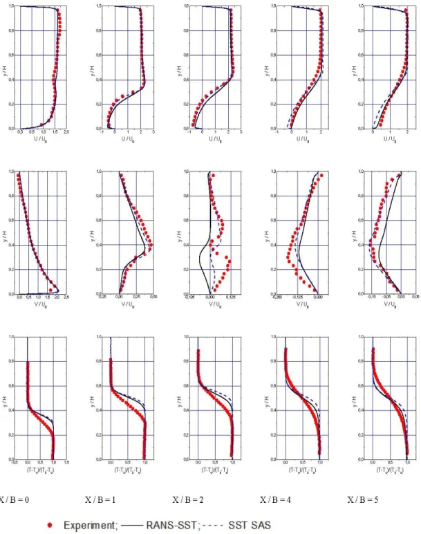
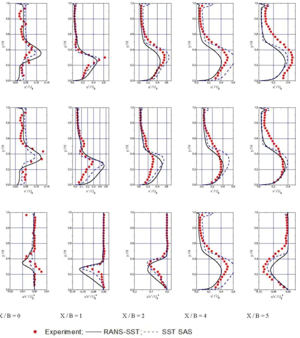
FIG. 4: Velocities, stresses, and temperatures at the longitudinal stations

91

7. RESULTS AND DISCUSSION 7.1 Validation

SST-RANS and SST-SAS time-averaged results, including the measurement data for comparison, are shown in Figs. 4 and 5. Globally, velocities, stresses, and thermal profiles at the five locations of the channel are qualitatively well reproduced by the two models. Comparing the two models, the SAS model is by far in better agreement with exper- imental data, especially for the three first measurement stations, while some discrepancy is observed in the two last ones. The reasons for this difference can be explained partly by low spatial and temporal resolution in regard to turbu- lence model requirements. Another source of discrepancy can be due to differences in the inlet boundary conditions

FIG. 5: Distribution of the fluctuations and shear stress at various longitudinal stations

92

between experiment and numerical runs. In fact, a fully developed velocity and high level of turbulence intensity are assumed at the inlet, whereas it is not clear if this is the case in experimental work. While the longitudinal velocity is well reproduced almost in all stations, the vertical velocity shows some considerable differences between the two models and the experimental data. For example, in station (x/B = 2), the qualitative experimental V /U0 profile is

slightly well captured by the SAS model, while the RANS model fails to reproduce the two positive values upper and lower the midline position (y/H = 4). Negative values reproduced by the RANS model and the weak positive value by the SAS model show that numerical results predict a smaller separation bubble compared to the experimental one. Turbulence intensity differences are also highlighted by remarkable differences between the experimental data and simulation results for longitudinal and vertical fluctuation profiles. Nevertheless, both models reproduce high turbulence activities in the lower part of the domain (less that y/H = 4), while the upper part is globally free from turbulence.

7.2 Flow and Thermal Field Description

All results described and discussed here are obtained from SAS computation. Instantaneous flow separation and typical developing vortex structures downstream of the T-junction at t = 1 s real-time are shown in Fig. 6.

The visualization is based on isosurfaces of the so-called Q-criteria, a function of vorticity and strain rate of the flow field. Figure 7 clearly shows that the SAS model can give more details for the irregular turbulent vortex structures forming immediately downstream of the T-junction and being convected with the flow along the main pipe.

SST

SAS

FIG. 6: Isosurfaces of the Q criteria colored by the longitudinal velocity, Q = 500 [s−2]

93

FIG. 7: Spanwise variation of the longitudinal flow velocity distribution U/U0

94

From the experimental data provided by Hirota et al. (2010), the hot flow entering the channel is separated at the downstream edge of the T-junction, forming a large separation bubble along the bottom wall of the main channel. The reattachment point is located nearly at four times the width of the branch after the last edge of the T-junction. The location of the reattachment point is confirmed by Fig. 7, showing the spanwise variation of the longitudinal flow velocity distribution where the gray regions correspond to reverse flow. The comparison to experimental data from Hirota et al. (2010) is fairly good, including the boundary layer reattachment point and the three-dimensional behavior of the flow development. When approaching the wall side (Z/A = 0.875) the height of the bubble decreases and the flow reattachment point moves in the negative direction. Streamwise evolution of cross-sectional distribution of U/U0 (left) and secondary flow velocities (right) are shown in Fig. 8.

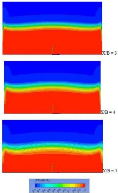
At the first station (x/B = 0), the upward direction is dominated over the cross section on the main channel, while at the second and third (x/B = 1 and 2, respectively) stations the upward flow becomes weaker. We remember here from previous figures that cross section x/B = 1 and 2 correspond to the bubble separation and x/B = 4 corresponds to the flow reattaching point. So, at x/B = 2, a longitudinal vortex develops near the lower corner, while it disappears at x/B = 4. This behavior is related to the streamline curvatures and the flow reattachment point. Streamwise evolution of the cross-sectional mean temperature normalized by the cold and hot flow temperatures are shown in Fig. 9.

X/B = 3

FIG. 8

95

X/B = 4

X/B = 5

FIG. 8: Streamwise evolution of cross-sectional distribution of U/U0 (left) and secondary flow velocities (right)

FIG. 9

96

FIG. 9: Streamwise evolution of the cross-sectional mean temperature distribution

The hot (bottom) and cold (top) regions are separated by the thermal mixing layer where the temperature vertical gradient (dT /dy) is at its maximal values. Surprisingly, and contrary to the 3D evolution stated before, the thermal field shows very nearly uniform distribution in the spanwise direction. This behavior is also reported by the exper- imental study of Hirota et al. (2010) and is explained by the fact that the longitudinal vortex is confined into the hot-flow region below the thermal mixing layer and does not exert any influence on the temperature distribution.

8. CONCLUSION

The T-junction experiment carried out at the Department of Mechanical Engineering of Mie University, Japan, is investigated here numerically with use of SST-RANS, SST-URANS, and SST-SAS models, the last one being in the framework of scale-resolving simulation gives LES-like results and still stays within the URANS strategy. Compared to SST-RANS, the SAS model has been shown to yield accurate results for this complex flow in the T-junction. The present study showed also that such quality results are very difficult to obtain using a URANS approach.

97

REFERENCES

Benhamadouche, S., Flow and heat transfer in a wall bounded pin matrix, In Proc. 15th ERCOFTAC/IAHR Workshop on Refined Turbulence Modelling, Chatou, France, 2011.

Braillard, O., Jarny, Y., and Balmigere, G., Thermal load determination in the mixing tee impacted by a turbulent flow generated by two fluids at large gap of temperature, The 13th Intl. Conf. on Nuclear Engineering (ICONE13-50361), Beijing, China, pp. 16–20, 2005.

Chapuliot, S., Gourdin, C., Payen, T., Magnaud, J.P., and Monavon, A., Hydro-thermal-mechanical analysis of thermal fatigue in a mixing tee, Nucl. Eng. Des., vol. 235, pp. 575–596, 2005.

Egorov, Y. and Menter, F., Development and Application of SST-SAS Turbulence Model in the DESIDER Project, Second Sym- posium on Hybrid RANS-LES Methods, Corfu, Greece, 2007.

Hirota, M., Mohri, E., Asano, H., and Goto, H., Experimental study on turbulent mixing process in cross-flow type T-junction, Int. J. Heat Fluid Flow, vol. 31, no. 5, pp. 776–784, 2010.

Hu, L.-W. and Kazimi, M.S., Large eddy simulation of water coolant thermal striping in a mixing tee junction, The 10th Intl. Topical Meeting on Nuclear Reactor Thermal Hydraulics (NURETH-10), Seoul, Korea, pp. 1–10, 2003.

Kitada, M., Asano, H., Kanbara, H., and Akaike, S., Development of automotive air conditioning system basic performance simulator: CFD technique development, JSAE Rev., vol. 21, pp. 91–96, 2000.

Menter, F.R., Zonal two equation k-ω turbulence models for aerodynamic flows, AIAA Paper No. 93–2906, Eloret Institute, Sunnyvale, 1993.

Menter, F.R. and Egorov, Y., A scale-adaptive simulations model using two-equation models, AIAA Paper No. 1095, 2005. Walker, C., Simiano, M., Zboray, R., and Prasser, H.-M., Investigations on mixing phenomena in single-phase flow in a T-junction

geometry, Nucl. Eng. Des., vol. 239, pp. 116–126, 2009.