HAL Id: hal-02372586
https://hal.archives-ouvertes.fr/hal-02372586
Submitted on 20 Nov 2019
HAL is a multi-disciplinary open access
archive for the deposit and dissemination of
sci-entific research documents, whether they are
pub-lished or not. The documents may come from
teaching and research institutions in France or
abroad, or from public or private research centers.
L’archive ouverte pluridisciplinaire HAL, est
destinée au dépôt et à la diffusion de documents
scientifiques de niveau recherche, publiés ou non,
émanant des établissements d’enseignement et de
recherche français ou étrangers, des laboratoires
publics ou privés.
Single Nanoparticle Growth from Nanoparticle Tracking
Analysis: From Monte Carlo Simulations to
Nanoparticle Electrogeneration
Vitor Brasiliense, Jean-Marc Noël, Kevin Wonner, Kristina Tschulik,
Catherine Combellas, Frederic Kanoufi
To cite this version:
Vitor Brasiliense, Jean-Marc Noël, Kevin Wonner, Kristina Tschulik, Catherine Combellas, et al..
Single Nanoparticle Growth from Nanoparticle Tracking Analysis: From Monte Carlo Simulations to
Nanoparticle Electrogeneration. ChemElectroChem, Weinheim : Wiley-VCH, 2018, 5 (20),
pp.3036-3043. �10.1002/celc.201800742�. �hal-02372586�
Reprint
A Journal of1 2 3 4 5 6 7 8 9 10 11 12 13 14 15 16 17 18 19 20 21 22 23 24 25 26 27 28 29 30 31 32 33 34 35 36 37 38 39 40 41 42 43 44 45 46 47 48 49 50 51 52 53 54 55 56 57
Single Nanoparticle Growth from Nanoparticle Tracking
Analysis: From Monte Carlo Simulations to Nanoparticle
Electrogeneration
Vitor Brasiliense,*
[a, b]Jean-Marc Noe¨l,
[a]Kevin Wonner,
[c]Kristina Tschulik,
[c]Catherine Combellas,
[a]and Fre´de´ric Kanoufi*
[a] By scrutinizing the trajectory of individual nanoparticles (NPs) in solution, NP tracking analysis (NTA) allows sizing individual NPs and providing meaningful complementary information to single NP electrochemistry. Herein, a model is developed to extend NTA to allow dynamic NP sizing and to analyze the kinetics of growth of NPs in solution. Interpreting the NP trajectories as scaled Brownian motion, Monte Carlo simulations produce stochastic trajectories of growing NPs (underdiffusion-con-trolled growth). These trajectories are grounds for determining a strategy to estimate the growth parameters of individual NPs from the time evolution analysis of the mean square displace-ment (MSD) curves. In particular, we evaluate the accuracy and precision of the parameter estimates from MSD analysis. In addition, the strategy is illustrated to depict the homogeneous electrosynthesis of silver NPs from the oxidation of a sacrificial Ag ultramicroelectrode (UME) in Fe2 + solution.
1. Introduction
The last decade has seen increasing interest in the interrogation of electrochemical behavior at the single NP level. It has been fueled by the development of ultrasensitive electroanalytical detection methods, such as NP impact electroanalysis (NIE), able to count and size individual NPs based on the measure-ment of stochastic current transients while the NPs collide at miniaturized electrodes.[1]Compared to ensemble averaged NP
measurements, usually performed on electrode-immobilized NPs, NIE not only gives a picture of charge transfer processes at the single entity level but it also adds new insights into transport phenomena, for example occurring in the vicinity of the electrode-electrolyte interface. Far beyond the implication of transport on molecular electrochemistry, NP electrochemistry is complexified because NPs are often larger than the tunneling distance to the electrode and comparable to or smaller than the viscous layer of the electrolyte. Most NIE and NTA experi-ments must therefore deal with complex NP transport when the NPs reach the vicinity of the electrode. Indeed,
experimen-tal evidences,[2,3] supported by Monte Carlo simulations,[4, 5]
show that during its excursion within the electrode area a single Ag NP may explore the tunneling region several times, leading to multiple reactive collisions, before it is fully oxidized. Moreover, other phoretic or directed motion of NPs to electro-des have been illustrated from such single NP electrochemical studies.[6,7] It generally shows the level of complexity brought
by the consideration of single NP transport into the charge transfer problem, explaining likely why NIE studies were mostly devoted to model reactions or model NP materials (e.g. electrocatalysis at Pt NPs, electrodissolution of Ag NPs). These studies provide promising means for scrutinizing also the chemistry of NPs in solution and highlight the advantages of complementing NIE studies by optical tracking of NPs motion for deriving dynamically chemical information.
Classical solutions to analyzing the motion of colloidal NPs in solution used various optical monitoring (light scattering or fluorescence).[8]These methods, performed most of the time ex
situ, complement NIE studies from indirect hydrodynamic sizing of particles. They address the flocculation of colloidal NPs solution in concentrated electrolytes.[9–13] The real time in situ
monitoring of individual NP transport during NIE studies was obtained by hyphenation of 2D or 3D high resolution (dark-field or fluorescence) optical microscopies[14–18] implemented
with spectroscopic monitoring.[19] They allowed studying how
the transport of NPs can be affected by the presence of a polarized collecting electrode.
If single NP electroanalytical studies have mostly focused on NP impacts on electrodes, electrochemical strategies have also been reported for the synthesis of NPs from the electro-generation of metal salt by the sacrificial oxidation of a metallic electrode in the presence of a solution-phase reducer.[20]It can
also be considered as a mean to chemically etch or transform NPs in solution from electrogenerated reactants.
[a] Dr. V. Brasiliense, Dr. J.-M. No[l, Dr. C. Combellas, Dr. F. Kanoufi Universit8 Sorbonne Paris Cit8, Universit8 Paris Diderot ITODYS, CNRS UMR 7086
15 rue Jean-Antoine de Ba"f, F-75013 Paris, France E-mail: [email protected]
[email protected] [b] Dr. V. Brasiliense
present address
Northwestern University Department of Chemistry 2145 Sheridan Rd., 60208 Evanston IL, USA E-mail: [email protected] [c] K. Wonner, Dr. K. Tschulik
Ruhr-University Bochum, Chair of Analytical Chemistry II and Centre for Electrochemical Sciences (CES), ZEMOS
Bochum 44801, Germany
Supporting information for this article is available on the WWW under https://doi.org/10.1002/celc.201800742
An invited contribution to a Special Issue on Single-Entity Electrochemistry
3036
ChemElectroChem 2018, 5, 3036–3043 T 2018 Wiley-VCH Verlag GmbH & Co. KGaA, Weinheim
Articles
1 2 3 4 5 6 7 8 9 10 11 12 13 14 15 16 17 18 19 20 21 22 23 24 25 26 27 28 29 30 31 32 33 34 35 36 37 38 39 40 41 42 43 44 45 46 47 48 49 50 51 52 53 54 55 56 57
We propose here a strategy to quantitatively depict such electrochemically generated process at the single entity level. While NIE may be inefficient to characterize the electrogenera-tion of NPs from an electrode, owing to the large current associated to reactant electrogeneration, we propose to rely on the inspection of NTA strategies. In this respect, a model is proposed to account for the growth of individual NPs during their reactive trajectory in solution. It considers the diffusion-controlled growth of NPs in solution (although not limited to such situation), characterized by two parameters: the NP size at the onset of the NP tracking, r0, and its growth rate, k. Monte
Carlo simulations are used to produce simulated stochastic trajectories of growing NPs which are analyzed through MSD curves. To evidence the time-evolution of the NP size, rp(t), and
extract the growth (r0 and k) from MSD curves, each NP
trajectory is divided into shorter sub-trajectories. Particular attention is given to the determination of minimum criteria for the applicability of the analysis (long enough trajectories, short enough sampling times), and optimization of the analysis parameters. Finally, the strategy is illustrated on an experimen-tal example where Ag NPs are electrogenerated in solution from the oxidation of a sacrificial Ag ultramicroelectrode, UME, in a reducing Fe2+solution.
2. Results and Discussion
2.1. Principle of the MSD Kinetic Analysis
We propose a strategy to extend the MSD analysis of the trajectory of constant size NPs, following Brownian motion, to growing (or dissolving) particles. Under pure Brownian motion (neither growth nor dissolution), the total displacement of a NP, during the time lapse Dt, can be described by a Gaussian random variable with zero mean and variance 2dDDt, where d is the dimensionality of the displacement (for a 2D trajectory d=2) and D is the diffusion coefficient of the NP. It follows that the MSD scales linearly with the elapsed time, proportionally to 2dD. Therefore, an estimation of MSD allows determination of D yielding, from Stokes-Einstein relationship (1), an estimate of the NP hydrodynamic radius r [Eq. (1)]:
D ¼ kBT
6phr ð1Þ
where kBis the Boltzmann’s constant, T the temperature and h
the viscosity of the solution.
The regular MSD analysis consists in assuming that time averages are equivalent to statistical averages, and taking the time-averaged mean square displacement (noted d2) as
estimator of hd2i ¼ 2dDDt. Implicitly, this procedure assumes
that the properties of the system (in particular D) do not evolve with time which does not hold for a growing particle.
This difficulty can be dealt with under the (much weaker) hypothesis that both time and statistical averages are commut-able, meaning that h d2 i ¼ hd2i: Then, the time-averaged
MSD curve is proportional to 2d(DDT, allowing measurement of
the averaged diffusion coefficient (D (from (1) the average particle size (r) during the measurement time. This is also corroborated by Monte Carlo simulations (described in the following section), which reveal only minor discrepancies between the diffusion coefficient as measured by time-averaged MSD analysis and the actual (D (typically <10%), as discussed in the supporting information, SI, section S1 and shown in Figure S1.
A corollary of this conclusion is that, in order to analyze the time-evolution of the size of a growing particle, one can analyze kinetically a long trajectory by separating it in concatenated sub-trajectories. The procedure is valid provided the original whole trajectory is long enough. This work describes how such trajectory segmentation can be used to describe the kinetics of NP growth in solution, focusing more particularly on a growth controlled by molecular diffusion from a solution phase, detailed in the next section. We then describe quantitatively the segmentation approach using Monte Carlo simulations. 2.2. Diffusion-Limited Growth
We focus on the case of diffusion limited growth of a NP of initial (at t=0) radius r0 and diffusion coefficient D0. The
transposition to other growth kinetics models is straightfor-ward. Similarly, the extension to dissolution of NPs is trivial, by considering negative values of the NP growth rate. In this diffusion limited case (DL), one assumes that the growth (dissolution, resp.) of a NP in solution is limited by diffusional transport of a molecular reactant, M, to (from, resp.) the NP surface. Owing to the small size of the growing NP, and the fast diffusion of the molecular reactants (typically DM~10@5–
10@6cm2/s) the diffusion layer develops quickly and a
steady-state is reached within less than a millisecond (~r02/DM, typically
0.1 ms for r0= 100 nm).
The growth dynamics of the radius, r(t), of an individual spherical NP under diffusion control can be obtained, as in previous works,[21] by considering the mass-transport limited
flux, j, of arrival of the reactant M (or leave of product for dissolution) at the NP. This flux is obtained by analogy to the mass-transport limiting current Ilim for the electrochemical
transformation of M (by 1-electron exchange) at a spherical nanoelectrode [Eq. (2)]:
Ilim=F ¼ 4pr2j ¼ 4p M½ ADMr ð2Þ
where F is the Faraday constant and [M] is the bulk concentration of the molecular species producing the NP of molecular volume Vm. The flux j can also be defined from the
change in NP volume, V [Eq. (3)] dV
dt ¼ Vm4p r
2j ð3Þ
The combination of Equations (2) and (3) yields Equa-tion (4):
3037
ChemElectroChem 2018, 5, 3036–3043 www.chemelectrochem.org T 2018 Wiley-VCH Verlag GmbH & Co. KGaA, Weinheim
1 2 3 4 5 6 7 8 9 10 11 12 13 14 15 16 17 18 19 20 21 22 23 24 25 26 27 28 29 30 31 32 33 34 35 36 37 38 39 40 41 42 43 44 45 46 47 48 49 50 51 52 53 54 55 56 57 dr dt¼ k4pr ð4Þ
where k=4pVmDM[M] within the present model corresponds to
the NP surface area growth rate, expressed in mm2/s. Assuming
that the particle has a radius r0 at the onset of its tracking
defined by time t=0, the solution of this differential equation is [Eq. (5)]: r2ð Þ ¼ rt 2 0: k2pt or r tð Þr 0 ¼ ffiffiffiffiffiffiffiffiffiffiffiffiffiffiffiffiffiffiffiffi 1 : k 2pr2 0 t r ð5Þ where the +or @sign corresponds to NP growth or dissolution respectively. This provides a model for the NP diffusion coefficient evolution, which is to be extracted from MSD analysis [Eq. (6)]: D tð Þ D0 ¼ ffiffiffiffiffiffiffiffiffiffiffiffiffiffiffiffiffi1 1 : k 2pr2 0t q ð6Þ
2.3. Monte Carlo Simulations
To test the precision of the segmentation approach, the trajectories of growing particles are simulated using Monte Carlo procedures. The simulation consists in discretizing the time in small time increments Dt (selected according to the sampling rate in experiments), and obtaining a sequence of positions for the NP from random variables simulating the processes at stake. In the present case, two physical processes affect the particle position: diffusion and growth. Diffusion is modeled as a stochastic process that determines the particle position. At each discrete time step ti (ti=ixDt), the ith time
increment after the trajectory onset, a direction and a displace-ment are randomly picked according to Brownian motion statistics.[22]
For a 3D motion, the direction is uniformly distributed on a unit-radius sphere (a unit circle for 2D motion, or between @1/ +1 occurrence for 1D random walk), while the displacement is chosen from a normally distributed random variable with zero mean and variance 2dD tð ÞDt. We particularly validate the Monte Carlo simulation by showing that for a constant value of the diffusion coefficient D0, the uniform distribution in the
sphere produces the classical MSD for a Brownian particle with a correct estimate of D0from the MSD slope.
The growth process is accounted for by updating the value of the diffusion coefficient. At each time step a new value of D(ti) is calculated from the growth kinetics model, and updated
accordingly. In the present case, (5) can be discretized and approximated by first-order Taylor expansion (with precision of order Dt) into (7), which yields the updated value of r(ti) from
its value at the preceding time step r(ti-1). As shown in Figure S2
in SI, the error introduced by the approximations is minimal [Eq. (7)].
r tð Þ ¼ r ti ði@1Þ þ k
4pr tði@1ÞDt ð7Þ
2.4. Anomalous Diffusion and Scaled Brownian Motion A large number of trajectories (ntraj=500) of growing NPs is
generated by this Monte Carlo procedure, with a same initial radius, r0, and growth rate, k. An example with a relatively slow
growth rate (k=0.01 mm2/s, r
0,=50 nm) is given in Figure 1. If
analyzed by the classical time-averaged MSD, d2, procedure, all
trajectories (blue lines in Figure 1A, with their average in red) show in a log-log representation an apparent Brownian motion. This allows extracting an apparent diffusion coefficient, (D; which characterizes the average size of the NPs, hd2i ¼ 2d(DDt.
By interpreting the motion as a Scaled Brownian Motion (SBM),[22,23] this hypothesis is indeed verified (for a detailed
justification see Section S3 in SI). Simply inferring the growth of the NPs directly from the time averaged MSD curves is then precluded, as it depends on two unknowns (r0and k).
For time-dependent situations, anomalous sub or super diffusion behavior may be observed, characterized by MSD varying as ta, with a<1 or >1 respectively.[8,23] The time
averaged MSD plots of the simulated growing NPs (Figure 1A), however, suggest a=1. This results from the change in NP size that can be seen as a continuous scaling of the diffusion coefficient compensating the change in the length or timescale of the movement (SBM). In other words the particle displace-ment can be written as the product of some scaling function [e.g. Eq. (6) here, see section S3 in SI] and a regular Brownian motion, which does not alter the intrinsic properties of the diffusion process. Moreover, the time averaged MSD analysis focuses on short time correlations, where the change in particle size is not expressive and anomalous effects are negligible.
The anomalous diffusion behavior can rather be expressed by averaging MSDs over a large number of NPs, providing a statistic representation, hd2i, given in Figure 1B. It provides a
Figure 1. Temporal (A) and statistic (B) MSDs in log–log plot of the Monte Carlo trajectories simulating the growth of NPs in solution. A) The temporal MSDs for each NP are obtained from their individual trajectories (red line: average of all trajectories). An average Brownian Motion is observed for all NPs (slope 1). B) Statistic MSD: for each time lag, d2is averaged over all NPs
trajectories. Two limiting behaviors are observed: pure diffusion at short timescale (red dashed line) replaced by sub-diffusion at longer times (black dashed line). Simulations of ntraj=500 trajectories of each Nt=5000
successive time steps of Dt=1/30s, D0=5 mm2/s (r0=50 nm) and
k=0.01 mm2/s.
3038
ChemElectroChem 2018, 5, 3036–3043 www.chemelectrochem.org T 2018 Wiley-VCH Verlag GmbH & Co. KGaA, Weinheim
1 2 3 4 5 6 7 8 9 10 11 12 13 14 15 16 17 18 19 20 21 22 23 24 25 26 27 28 29 30 31 32 33 34 35 36 37 38 39 40 41 42 43 44 45 46 47 48 49 50 51 52 53 54 55 56 57
full expression of the time-variation of the MSD, which can depict the dynamics of the competing transport and reaction processes,[24]for example described by the dimensionless eq. 6.
Typically in the statistic MSD presented in Figure 1B, the NPs are freely diffusing (slope a=1) at short times with a diffusion coefficient consistent with their initial size (or size in the absence of growth), r0. While for longer times the displacement
of the NPs becomes anomalous (a<1), the MSD follows a t1/2
evolution (slope a=1=
2). The latter is consistent with the long
time limit of eq. 6 (D tð Þ ' D0r0
ffiffiffiffiffiffiffiffiffiffiffiffiffi 2p=kt p yielding hd2i varying as ffiffiffiffiffiffiffi t=k p
). These two limiting behaviors depend on a characteristic time, t & 2pr2
0=k, representing the dynamics of the growth
process: for t <0.3t the MSD is Brownian; it becomes anomalous above and fully governed by the growth dynamics for t >3t. These limiting behaviors can be used, for large number of trajectories, to extract both r0 and the growth rate
at short and long time respectively from the MSD slopes. Even though insightful, this strategy requires that all trajectories are obtained for NPs possessing the same initial radius at the start of the tracking procedure, which is rather difficult to obtain experimentally.
2.5. Kinetic MSD Analysis of Monte Carlo Simulated Curves To extract kinetic information from the trajectories of individual NPs, individual trajectories are submitted to the kinetic mean square displacement (KMSD) analysis procedure illustrated in
Figure 2, for example with a fast growth rate. The simulated trajectories, of length Nt, are segmented into sub-segmented
trajectories (either correlated or uncorrelated, see comparison in section S4 in SI), corresponding to subsequences of Ns(Ns<
Nt) consecutive time steps. The key idea of the KMSD method is
to perform a MSD analysis in each of these sub-segments. In the segmentation procedure, each individual trajectory is divided into nseg=Nt@Ns+1 sub-segmented trajectories. For
1,k,nseg the MSD analysis performed within the kth
sub-segment of duration NsDt starting at tk=(k@1)Dt and ending at
tk+NsDt allows estimating the average NP diffusion coefficient
(and corresponding size) for the average time of the sub-segment tk’=tk+NsDt/2 yielding D(tk’) and r(tk’)). For example in
Figure 1B, a trajectory consisting of Ntot=300 points, is
segmented into nseg=241 intermediate trajectories of Ns=60
points. The MSD analysis performed on the first segment of Ns=60 points will provide an average diffusion coefficient D(t1’)
during the first fifth of the overall trajectory. Equivalently, the last MSD over the last 60 points will generate an average diffusion coefficient (D(t241’)) on the last fifth of the overall
trajectory.
The precision of each estimated D(tk’) and r(tk’) depends on
the number of points per sub-segment, and therefore Ns is
critical to determine the precision and resolution of KMSD methods. A tradeoff between the precision and temporal resolution is to be observed: smaller values of Nsallow a higher
number of sub-segments to be estimated (high value of nseg
and therefore of temporal resolution), but each point is less precisely estimated, introducing random noise and decreasing the fitting performance.
An estimation of the procedure precision is given in Figure 2B,C by analyzing 300 Monte Carlo generated trajecto-ries. Figure 2B shows the distributions of all values of NP radii, r(tk’), from all the 300 trajectories simulated with a unique set of
(r0, k) parameters. These values of r(tk’) are compared to the
expected time-variation given by eq. 5. The 50thpercentile (the
median) of the distribution for each given time tk’ is a
meaningful estimate of the true value of r(tk’) for a large
population of identical particles. For each time, t’k, the r(tk
’)-distributions are all centered at the true value of r(tk’), indicating
that the method is unbiased (distributions shown in section S5 in SI). From the obtained curves, r0is determined by the first
estimation of rðti), while k is evaluated by a one-parameter fit
of eq. 5, performed using least-squares. Figure 2C shows two examples of such r(tk’) plot for two given trajectories with their
best fit (red curves). The distribution of the fitted values of growth parameter, k, for the whole 300 Monte Carlo trajectories is given in Figure 2D.
2.6. Error Estimation on Individual NP Growth Parameters A crucial point in single entity analysis is how the stochasticity impacts the distribution of behavior observed and to what extent the diversity of size or of kinetic behavior can be estimated meaningfully from the behavior of single entities. Our ability to detect this diversity of behavior, however, Figure 2. A) Procedure of segmentation of a given trajectory by overlapping
sub-segments: within each sub-segment (arrow between vertical bars) an instantaneous diffusion coefficient D(t’k) is estimated yielding, in (B), the
evaluation of the discretized time-evolution of r. B) Application to 300 Monte Carlo simulated trajectories. Each green dot on the graph represents one estimate of r at the different average time of the sub-segment. The dashed lines represent from top to bottom the 95th, 75th, 50th; 25th, 5thpercentiles of
the distribution. The analytical solution given by Equation (5) (red line) agrees with the median, showing that the method is not biased. The parameters used for the simulations are Nt=300, Ns=60 steps, Dt=0.033 s
with D0¼ 5 mm2=s and k ¼ 0:1 mm2=s. C) Two examples of r(t) evolutions
(fits in red) from two trajectories with the same parameters. D) Distribution of the growth rate k obtained from the fit of the r(t) evolutions. The distribution fitted by a Student-law yields k ¼ 0:10 : 0:04 mm2=s.
3039
ChemElectroChem 2018, 5, 3036–3043 www.chemelectrochem.org T 2018 Wiley-VCH Verlag GmbH & Co. KGaA, Weinheim
1 2 3 4 5 6 7 8 9 10 11 12 13 14 15 16 17 18 19 20 21 22 23 24 25 26 27 28 29 30 31 32 33 34 35 36 37 38 39 40 41 42 43 44 45 46 47 48 49 50 51 52 53 54 55 56 57
depends on the precision of the determination of ðr0; kÞ pair.
From the standard deviation s of each measurement r, and from the values of r0 and k extracted from the fit, one can
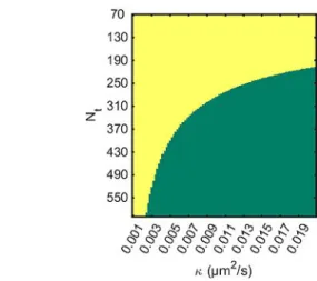
determine the standard deviation of k (details in S5 in SI) [Eq. (8)]: SD kð Þ & ffiffiffiffiffiffiffiffiffiffiffiffi1 Nt=Ns p 2p ðNt@ NsÞDt 2 s ffiffiffiffiffiffiffiffiffiffiffiffiffiffiffiffiffiffiffiffiffiffiffiffiffiffiffiffiffiffiffiffiffiffiffiffiffi 2s2þ 2r2 0þ kN2ptDt r ð8Þ and therefore the accuracy of the MSD procedure to analyze NP growth from single NP trajectory tracking. We can statistically determine meaningful growth as long as the measured k is larger than 2 standard deviations, that is, if k > 2 StDev kð Þ, which is equivalent to requiring a signal to noise ratio higher than 2. Based on this criterion, eq. 8 predicts a required minimum number of steps for detecting growth on a single particle basis, as illustrated in Figure 3. For slow growth,
multiple trajectories are required, reducing the standard deviations by a factor ffiffiffiffiffiffiffipntraj, and allowing it to pass into the
green region.
For all experimentally relevant parameters, however, good agreement was found between eq. 8 and robust estimators of the standard deviation of the distribution (inter-quartile range). Up to this point, the KMSD method can reliably be applied on MC simulations if the kinetic parameter, k, and the trajectory range, Ns, are high enough. The natural next step is to put the
method on trial over experimental results. In the next section, the capabilities of the method are showcased by studying the homogeneous growth kinetics of silver NPs in the vicinity of a microelectrode.
2.7. Application of KMSD to Experimental Results: Ag NP Homogeneous Growth
2.7.1. Probing Electrogenerated NPs by Electrochemical Nanoimpacts
To illustrate the model proposed, the electrogeneration and tracking of Ag NPs from a sacrificial Ag UME (experimental details in section S6 in SI) was monitored in situ and real time by high resolution 2D dark-field optical microscopy. The anodic dissolution of a sacrificial Ag UME is obtained by polarizing it at potentials allowing the conversion of the Ag UME into Ag+
ions. The UME is then used as a local source of Ag+ ions, but
here, as sketched in Figure 4A, in a solution of an electron
donor (Fe2+, E0
Fe3+/Fe2+=0.77 V, E0Ag +/Ag=0.80 V vs NHE). Owing
to their E0, Reaction (9) between the electrogenerated Ag+and
Fe2+ yields the production of metallic Ag, and therefore the
birth of Ag NPs in solution.
Agþþ Fe2þ !Ag0þ Fe3þ ð9Þ
Figure 4B presents the linear sweep voltammograms (LSVs) recorded at the Ag UME without and with 50 mM Fe2 +. Without
Fe2+ the oxidation peak centered at 0.5 V vs Ag/AgCl reveals
the Ag!Ag+oxidation and UME dissolution. In the presence of
Fe2+ a noisy, plateau-like feature attributed to the Fe2+!Fe3 +
oxidation appears at more anodic potentials. This shows the occurrence of multiple stochastic current spikes reminiscent of the electrochemical collision and dissolution of individual Ag
NPs.[2,4] Indeed, spikes are detected at potentials allowing the
Ag UME dissolution and only in the presence of Fe2 + since no
spike was observed without Fe2+ (Figure S8 in SI) ; then, if
metal NPs are formed in solution their oxidative dissolution can be detected while they are diffusing back and colliding the UME.
The first direct evidence of the electrosynthesis of Ag NPs is given by ex situ SEM imaging (Figure 5A) complemented by EDX analysis (Figure S9 in SI). Pure Ag nanocubes (NCs, edge length, l=317:80 nm) are detected on the insulating glass surrounding the Ag UME, after applying a 10s pulse at 0.7 V. The homogeneous phase synthesis of Ag NCs generally requires Figure 3. Minimal length of trajectory (in number of points, Nt) for detecting
NPs growth based on a single trajectory (segment length: Ns=60, Dt =1/
30 s). In the green region a single trajectory is in principle enough to assert growth, while for shorter trajectories, averaging over multiple trajectories is required.
Figure 4. A) Principle of Ag NPs electrosynthesis by electrodissolution of an Ag UME. B) Linear sweep voltammograms of the oxidation of an a =12.5 mm radius Ag UME in 0.05 M KPF6(aq) before (–) and after (–) addition of 50 mM
FeSO4·7H2O; scan rate: 50 mV s@1.
3040
ChemElectroChem 2018, 5, 3036–3043 www.chemelectrochem.org T 2018 Wiley-VCH Verlag GmbH & Co. KGaA, Weinheim
1 2 3 4 5 6 7 8 9 10 11 12 13 14 15 16 17 18 19 20 21 22 23 24 25 26 27 28 29 30 31 32 33 34 35 36 37 38 39 40 41 42 43 44 45 46 47 48 49 50 51 52 53 54 55 56 57
concentrated Ag+ solutions.[25] This is provided here, at the
applied potential, from the UME current (up to 150 nA); the UME surface allows an equivalent release of up to 20 mM Ag+
ions (Figure 4B). Moreover, the UME is not only locally generating concentration gradient of Ag+ ions, but it is
oxidizing Fe2 + to Fe3 +. This is also in favor of Ag NC formation
since Fe3+ is a known oxidative etchant of metallic Ag allowing
the synthesis of Ag NCs from Ag+ solution,[26] or from the
solution phase reduction of octahedral AgCl. The electrosyn-thesis conditions provide a mixture of Fe3 +, Fe2 + and Ag+ in
the UME vicinity favoring the growth of preferential facets, explaining the electrogeneration of NCs. The morphology of the Ag NPs will be the subject of a forthcoming paper.
Further insights in this electrosynthesis process are pro-vided from single NPs sizing and counting. In a closer examination of the oxidative current spikes recorded during an anodic potential step at a Ag UME (Figure 5B–D and Figure S10 in SI), we assume i) that each spike corresponds to the event of
one Ag NC impacting the UME, leading to ii) the complete NP oxidative dissolution (even though questionable for such large
NPs[2–4]). Then the charge, Q, associated to each spike provides
an electrochemical rough estimate of the cube edge length, lEC,
of individual NCs from [Eq. (10)]: lEC¼ ffiffiffiffiffiffiffiffiffi QVm F 3 r ð10Þ with Vm=10.27 cm3/mol, the molar volume of Ag.
The electrochemical collisions extracted from a first 2 s interval of the chronoamperogram (zoom in Figure 5B) yield lEC=300 nm, while the average charge (and size) of the collision
increases with time (Figure 5C), suggesting the particles are growing during the process until their size stabilizes around lEC=590 nm. The impact frequency, f, also increases with the
synthesis time (Figure 5D). f provides a rough estimate of the concentration of the NCs, [NC], at few micrometers from the UME, by Equation (11):
f ¼ 4DAg½NCAa ð11Þ
with DAg the average diffusion coefficient of the Ag NC.
Assuming a 300 nm NC has an average DAgof ca. 1 mm2s@1, the
initial frequency of 10 impacts per second suggests that the UME has generated a concentration of 2x10¹¹NPs/mL solution,
which increases 5-fold between the beginning and the end of the experiment. In this single NIE the UME only senses the limited proportion of the NCs produced in its vicinity and which can return to it, that is within a diffusion length of ca. (2DAgt)1/2.
Typically, during the 10s of the chronoamperogram a 300 nm cube would have diffused <5 mm before it is detected. This electrochemical analysis therefore partially addresses the NP growth process taking place in the close vicinity of the UME. 2.7.2. From Optical Monitoring to MSD Dynamic Sizing Dark field optical microscopy allows the in situ monitoring of NP formation at longer distances from the UME. For that purpose, an Ag UME was positioned in a drop cell, mounted on a thin glass slide on top of an inverted microscope. This assembly allows focusing on the apex of the UME, then imaged with a CCD camera (up to 30 frames per second) under dark-field illumination through a dark-dark-field condenser. Video S1 shows the 2D optical monitoring of the solution surrounding the Ag UME biased at 0.3 V in a 1 mM Fe2 +solution. These less
oxidizing potential and lower reducer content were chosen to generate a lower amount of NCs (improved resolution), compared to the conditions of Figure 5B: the UME current, ca. 40 nA, corresponds to a local release of 5 mM Ag+ ions. The
oxidation of the UME starts from the third second of the video, and immediately after that, bright spots are distributed in solution, within a hemisphere of radius between 50 and 100 mm from the center of the Ag wire (Figure 6A). These bright spots, attributed to Ag NPs, confirm the generation of NPs in solution upon electrochemical actuation. In controlled bulk Figure 5. Electrosynthesis of Ag NCs from the oxidation of a sacrificial Ag
UME inspected ex situ by SEM (A) or in situ by NIE (B–D). A) SEM image of the glass part of the apex of the UME after a 10s pulse (0.7 V vs Ag/AgCl). Inset: NC length edge distribution. B) Nanoimpacts of electrosynthesized Ag NCs during a 0.7 V pulse. Inset: NPs size distribution inferred from individual electrochemical spikes. C,D) Time evolution of spikes charge and frequency.
3041
ChemElectroChem 2018, 5, 3036–3043 www.chemelectrochem.org T 2018 Wiley-VCH Verlag GmbH & Co. KGaA, Weinheim
1 2 3 4 5 6 7 8 9 10 11 12 13 14 15 16 17 18 19 20 21 22 23 24 25 26 27 28 29 30 31 32 33 34 35 36 37 38 39 40 41 42 43 44 45 46 47 48 49 50 51 52 53 54 55 56 57
experiments, solutions of Ag+ ions at comparable 5 mM
concentration in 50 mM KPF6 in the presence or absence of
Fe2+ ions were imaged by dark field microscopy (Figure S11 in
SI). They produced respectively either many (>100) Ag NPs (no SEM analysis) or <10 scattering features confirming that the generation of Ag NPs most likely results from Ag+ reduction. A
further control experiment of the sacrificial electrodissolution of the Ag UME into Ag+ ions in a KPF
6solution in the absence of
Fe2+ ions (video S2 and red trace transient in Figure S8 in SI)
shows the possible formation of only few NPs with much slower dynamics likely indicative of the slow photoreduction of Ag+ or silver salt nanocrystals. Again this slower dynamics
further supports that the optical process depicted in Figure 6A corresponds to the solution phase reduction of Ag+ ions into
Ag NCs.
To quantitatively evaluate the homogeneous-phase syn-thesis at the single particle level, ntraj=250 different Ag NPs
were tracked from the successive frames of the movie (video S1). It gives rise to ntraj=250 individual trajectories of individual
Ag NPs (with at least Nt=100 time steps per trajectory for each
250 NPs). The statistic MSD analysis, proposed in the theoretical section, through averaging over a large number of NPs, is not experimentally meaningful here since all NPs cannot be detected with the same initial size. Our procedure rather relies on the analysis of the temporal MSDs of these 250 different NPs
trajectories. Examples of experimental temporal MSDs of some of these NPs are plotted in a log-log scale versus the time lag, tlag, in Figure 6B (blue curves). These experimental MSD curves
reproduce nicely the simulated trajectories (red curves) and confirm the predicted average Brownian behavior.
Each individual NP trajectory was then analyzed by the KMSD procedure, vide supra. Each experimental trajectory was segmented in shorter trajectories allowing instantaneous estimates of each individual NP apparent hydrodynamic radius rAgvalue r(t) at different times during the course of its trajectory.
An example of instantaneous evolution of r(t), given in Figure 6C, shows that the NP is growing during its tracking. The distribution of the average radius, rm, of the different NPs
(Figure 6E), estimated over each trajectory is in good agree-ment with the size distribution of the NPs estimated ex situ by SEM (even though rm corresponds to the NP hydrodynamic
radius). Similarly a distribution of the individual NP growth rate estimated from each individual r(t) fit was obtained (Figure 6D), giving k=0.008:0.004 mm2s@1, where the error is estimated
using the interquartile differences. The distribution of k values is rather large as also predicted and explained in the theoretical part. Particularly for such low value of k, it is statistically sound to obtain negative values of k, which are also observed with similar probability during the Monte Carlo simulation reproduc-ing this experimental growth process (red distribution in Figure S5.2 in SI). As discussed in the theoretical part, longer trajectories should be preferred, even though experimentally difficult here owing to both the experiment duration and the limited camera acquisition rate. Based on the proposed solution-phase growth model, k =4pDsolCbVm, with a process
controlled by diffusion of the Fe2 + limiting species, D
soland Cb
being the diffusion coefficient and local bulk concentration of Fe2+, respectively. The distribution of k yields values of Cbin the
mM range, which agrees reasonably with the 1 mM bulk concentration and further supports that the NPs are growing within the diffusion field of the UME.
3. Conclusions
Electrochemistry in single entity studies is not only an analytical platform but it can also be used to electrogenerate dispersed NPs. To depict the NP production process, one can rely on the optical tracking of their individual trajectory in solution. Monte Carlo procedures allow simulating trajectories of NPs growing in solution under mass-transfer control. These simulated stochastic trajectories are analyzed to quantitatively describe the NP growth mechanism (growth rate constant).
It is shown that standard mean-square displacement analysis conventionally used to characterize pure Brownian particle also applies to such NPs (described by a time-depend-ent diffusion coefficitime-depend-ent, allowing an estimate of the average diffusion coefficient during the trajectory), but the particle growth cannot be identified from such conventional approach. The latter process can be identified from statistic averaging over a large number of NPs or by segmenting each single NP trajectory into sub-segments providing instantaneous NP size Figure 6. A) Dark field optical image (from Video S1) taken at the apex of a
Ag UME 10s after the application of E=0.3 V; 1 mM Fe2 ++50 mM KPF 6(aq).
B) Comparison between the time-averaged MSD analysis of individual NP trajectories and simulations using the parameters obtained through the kinetic-MSD segmentation (blue: experimental, red: simulated). C) Example of a single NP instantaneous radius evolution with time (blue: experimental, red: fit) using the best-fit parameters D,E) Distribution of the values of respectively k and average radius rmestimated from the KMSD analysis of
each trajectory.
3042
ChemElectroChem 2018, 5, 3036–3043 www.chemelectrochem.org T 2018 Wiley-VCH Verlag GmbH & Co. KGaA, Weinheim
1 2 3 4 5 6 7 8 9 10 11 12 13 14 15 16 17 18 19 20 21 22 23 24 25 26 27 28 29 30 31 32 33 34 35 36 37 38 39 40 41 42 43 44 45 46 47 48 49 50 51 52 53 54 55 56 57
estimates, r(t). The fit of r(t) by appropriate model allows quantifying the growth kinetics at the single NP level. The model is successfully applied to the monitoring of the electro-generation of single Ag nanocubes from the electrodissolution of a sacrificial Ag UME in a solution of a reducer.
Acknowledgements
This work was financially supported by the Agence Nationale pour la Recherche (NEOCASTIP ANR-15-CE09-0015-02 project, FK) and by the Cluster of Excellence RESOLV (EXC 1069) funded by the German Research Foundation (DFG) and by a “NRW Ru¨ckkehrer-programm” Fellowship of the State of North-Rhine Westphalia (KT and KW).
Conflict of Interest
The authors declare no conflict of interest.
Keywords: MSD · nanoparticle tracking analysis · growth dynamics · nanoparticle electrosynthesis
[1] a) K. J. Stevenson, K. Tschulik, Curr. Opin. Electrochem. 2017, 6, 38–45; b) S. V. Sokolov, S. Eloul, E. K-telhçn, C. Batchelor-McAuley, R. G. Compton, Phys. Chem. Chem. Phys. 2017, 6, 28–34; c) T. J. Anderson, B. Zhang, Acc. Chem. Res. 2016, 49, 2625–2631.
[2] S. M. Oja, D. A. Robinson, N. J. Vitti, M. A. Andrews, Y. Liu, H. S. White, B. Zhang, J. Am. Chem. Soc. 2017, 139, 708–718.
[3] J. Ustarroz, M. Kang, E. Bullions, P. R. Unwin, Chem. Sci. 2017, 8, 1841– 1853.
[4] W. Ma, H. Ma, J.-F. Chen, Y. Y. Peng, Z. Y. Yang, H. F. Wang, Y. L. Ying, H. Tian, Y. T. Long, Chem. Sci. 2017, 8, 1854–1861.
[5] D. A. Robinson, Y. Liu, M. A. Edwards, N. J. Vitti, S. M. Oja, B. Zhang, H. S. White, J. Am. Chem. Soc. 2017, 139, 16923–16931.
[6] a) S. E. Fodsick, M. J. Anderson, E. G. Nettleton, R. M. Crooks, J. Am. Chem. Soc. 2013, 135, 5994–5997; b) A. Boika, A. J. Bard, Anal. Chem. 2014, 86, 11666–11672; c) M. Kang, D. Perry, Y.-R. Kim, A. W. Colburn, R. A. Lazenby, P. R Unwin, J. Am. Chem. Soc. 2015, 137, 10902–10905; d) J. F. Sheng, M. Pumera, ACS Sens. 2016, 1, 949–957.
[7] A. N. Patel, A. Martinez-Marrades, V. Brasiliense, D. Koshelev, M. Besbes, R. Kuszelewicz, C. Combellas, G. Tessier, F. Kanoufi, Nano Lett. 2015, 15, 6454–6463.
[8] a) H; Shen, L. J. Tauzin, R. Baiyasi, W. Wang, N. Moringo, B. Shuang, C. F. Landes, Chem. Rev. 2017, 117, 7331–7376; b) C. Manzo, M. F.
Garcia-Parajo, Rep. Prog. Phys. 2015, 78, 124601; c) H. Qian, M. P. Sheetz, E. L. Elson, Biophys. J. 1991, 60, 910–921.
[9] J. C. Lees, L. Ellison, C. Batchelor-McAuley, K. Tschulik, C. Damm, D. Omanovic, R. G. Compton, ChemPhysChem 2013, 14, 3895–3897. [10] S. V. Sokolov, K. Tschulik, C. Batchelor-McAuley, K. Jurkschat, R. G.
Compton, Anal. Chem. 2015, 87, 10033–10039.
[11] A. Fernando, P. Chhetri, K. K. Barakoti, S. Parajuli, R. Kazemi, M. A. Alpuche-Aviles, J. Electrochem. Soc. 2016, 163, H3025–H3031.
[12] D. A. Robinson, A. M. Kondajji, A. D. Castaneda, R. Dasari, R. M. Crooks, K. J. Stevenson, J. Phys. Chem. Lett. 2016, 7, 2512–2517.
[13] S. E. F. Klein, B. Serrano-Bou, A. I. Yanson, M. T. M. Koper, Langmuir 2013, 29, 2054–2064.
[14] K. Hill, S. Pan, J. Am. Chem. Soc. 2013, 135, 17250–17253.
[15] a) W. Wo, Z.. Li, Y. Jiang, M. Li, Y. W. Su, W. Wang, N. Tao, Anal. Chem. 2016, 88, 2380–2385; b) Y. Fang, W. Wang, X. Wo, Y. Luo, S. Yin, Y. Wang, X. Shan, N. Tao, J. Am. Chem. Soc. 2014, 136, 12584–12587.
[16] a) V. Brasiliense, A. N. Patel, A. Martinez-Marades, J. Shi, Y. Chen, C. Combellas, G. Tessier, F. Kanoufi. , J. Am. Chem. Soc. 2016, 138, 3478– 3483. b) V. Brasiliense, P. Berto, C. Combellas, G. Tessier, F. Kanoufi, Acc. Chem. Res. 2016, 49, 2049–2057.
[17] Y. Yu, V. Sundaresan, S. Bandyopadhyay, Y. Zhang, M. A. Edwards, K. McKelvey, H. S. White, K. A. Willets, ACS Nano 2017, 11, 10529–10538. [18] S. E. Fodsick, M. J. Anderson, E. G. Nettleton, R. M. Crooks, J. Am. Chem.
Soc. 2013, 135, 5994–5997.
[19] a) V. Brasiliense, P. Berto, R. Kuszelewicz, C. Combellas, G. Tessier, F. Kanoufi, Faraday Discuss. 2016, 193, 339–352; b) K. Wonner, M. V. Evers, K. Tschulik, J. Am. Chem. Soc. 2018, doi:10.1021/jacs.8b02367.
[20] a) M. T. Reetz, W. Helbig, J. Am. Chem. Soc. 1994, 116, 7401–7402; b) M. T. Reetz, S. A. Quaiser Angew. Chem. Int. Ed. 1995, 56, 2240–2241; c) N. Vilar-Vidal, M. Carmen Blanco, M. A. Lopez-Quintela, J. Rivas, C. Serra, J. Phys. Chem. C 2010, 114, 15924–15930; d) B. S. Gonzalez, M. C. Blanco, M. A. Lopez-Quintela, Nanoscale 2012, 4, 7632–7635; e) G. R. Nasretdinova, R. R. Fazleeva, R. K. Mukhitova, I. R. Nizameev, M. K. Kadirov, A. Y. Ziganshina, V. V. Yanilkin Electrochem. Commun. 2015, 50, 69–72; f) J. H. Bae, R. F. Brocenschi, K. Kisslinger, H. L. Xin, M. V. Mirkin, Anal. Chem. 2017, 89, 12618–12621.
[21] H. S. Toh, C. Batchelor-McAuley, K. Tschulik, M. Uhlemann, A. Crossley, R. G. Compton, Nanoscale 2013, 5, 4884–4893.
[22] U. F. Wiersema, Ed. , in Brownian Motion Calculus, John Wiley and Sons, Chichester, 2008, pp 36, 93 and 147.
[23] J. H. Jeon, A. V. Chechkin, R. Metzler, Phys. Chem. Chem. Phys. 2014, 16, 15811–15817.
[24] F. Hçfling, T. Franosch, E. Frey, Phys. Rev. Lett. 2006, 96, 165901–165904. [25] a) S. Zhou, J. Li, K. D. Gilroy, J. Tao, C. Zhu, X. Yang, X. Sun, Y. Xia, ACS Nano 2016, 10, 9861–9870; b) Y. Sun, Y. Xia, Science 2002, 298, 2176– 2179.
[26] Y. Ma, W. Li, J. Zeng, M. McKiernan, Z. Xie, Y. Xia, J. Mater. Chem. 2010, 20, 3586–3589.
Manuscript received: June 4, 2018 Accepted Article published: July 18, 2018 Version of record online: August 1, 2018
3043
ChemElectroChem 2018, 5, 3036–3043 www.chemelectrochem.org T 2018 Wiley-VCH Verlag GmbH & Co. KGaA, Weinheim