The length of the world’s glaciers – a new approach for the global calculation of center lines

www.the-cryosphere.net/8/1741/2014/ doi:10.5194/tc-8-1741-2014

© Author(s) 2014. CC Attribution 3.0 License.

The length of the world’s glaciers – a new approach for the global

calculation of center lines

H. Machguth1and M. Huss2,3

1_{Arctic Technology Center, Technical University of Denmark, Kgs. Lyngby, Denmark} 2_{Department of Geosciences, University of Fribourg, Fribourg, Switzerland}

3_{Laboratory of Hydraulics, Hydrology and Glaciology (VAW), ETH Zurich, Zurich, Switzerland}

Correspondence to: H. Machguth (homac@byg.dtu.dk)

Received: 3 April 2014 – Published in The Cryosphere Discuss.: 14 May 2014 Revised: 4 August 2014 – Accepted: 6 August 2014 – Published: 19 September 2014

Abstract. Glacier length is an important measure of glacier geometry. Nevertheless, global glacier inventories are mostly lacking length data. Only recently semi-automated ap-proaches to measure glacier length have been developed and applied regionally. Here we present a first global assess-ment of glacier length using an automated method that re-lies on glacier surface slope, distance to the glacier margins and a set of trade-off functions. The method is developed for East Greenland, evaluated for East Greenland as well as for Alaska and eventually applied to all ∼ 200 000 glaciers around the globe. The evaluation highlights accurately cal-culated glacier length where digital elevation model (DEM) quality is high (East Greenland) and limited accuracy on low-quality DEMs (parts of Alaska). Measured length of very small glaciers is subject to a certain level of ambiguity. The global calculation shows that only about 1.5 % of all glaciers are longer than 10 km, with Bering Glacier (Alaska/Canada) being the longest glacier in the world at a length of 196 km. Based on the output of our algorithm we derive global and re-gional area–length scaling laws. Differences among rere-gional scaling parameters appear to be related to characteristics of topography and glacier mass balance. The present study adds glacier length as a key parameter to global glacier invento-ries. Global and regional scaling laws might prove beneficial in conceptual glacier models.

1 Introduction

Glacier length is one of the central measures representing the geometry of glaciers. Changes in climate have a delayed but

very clear impact on glacier length, and the advance or re-treat of glaciers is frequently used to communicate observed changes to a broader public. In a scientific context, glacier length change records are interpreted with respect to varia-tions in climate (e.g., Hoelzle et al., 2003; Oerlemans, 2005). Despite being scientifically relevant and easy to communi-cate, glacier length is difficult to define and has been mea-sured only for a relatively small number of glaciers world-wide (Cogley, 2009; Paul et al., 2009; Leclercq et al., 2014). Several authors have defined glacier length as the length of the longest flow line of a glacier (e.g., Nussbaumer et al., 2007; Paul et al., 2009; Leclercq et al., 2012). Such a concept is reasonable because of linking length to glacier flow, one of the basic processes controlling the geometry of glaciers. But defining the longest flow line on a glacier is a nontriv-ial task because ice forming in the upper accumulation area travels close to the glacier bed towards the tongue. Thus, the longest flow line is located somewhere close to the bottom of the glacier, while flow trajectories of surface particles never extend over the full length of a glacier. Then again glacier length generally refers to the glacier surface represented on a map, a satellite image or in reality. Hence, glacier length as a surface measure can only be linked indirectly to the three-dimensional process of glacier flow.

In the past, glacier length was determined manually in a laborious way. Automated computation of glacier length has gained new relevance with the advent of the Randolph Glacier Inventory (RGI), a worldwide data set of glacier polygons (Pfeffer et al., 2014). While other geometric pa-rameters such as area, elevation and slope can be automat-ically derived from glacier polygons and digital elevation

models (DEMs), until recently no automated approach ex-isted to measure glacier length. The requirements for such an approach should be based on the definition of glacier length given above but also need to address practical issues: the method should (i) mimic glacier flow, (ii) be computation-ally efficient, (iii) be fully automated and (iv) be able to deal with inaccurate DEM data. The requirements (ii) to (vi) re-sult from the need to apply the method to large-scale glacier inventories with limitations in quality of the input data.

Two recent studies by Le Bris and Paul (2013) and Kien-holz et al. (2014) presented semi-automatic approaches to de-rive glacier length and demonstrated the methods in local or regional applications. Le Bris and Paul (2013) suggest deter-mining the highest and lowest point of a glacier. A line con-necting the two points is drawn in such a way that distance to the glacier margins is maximized and downhill flow is re-spected. Kienholz et al. (2014) introduced the term “center line” and base their approach on the same principle of maxi-mizing the distance to the glacier margin. Elevation is consid-ered as a second criterion, and both conditions are combined by minimizing the costs on a cost grid.

The approach by Le Bris and Paul (2013) has the advan-tage that limitations in DEM quality have little influence on the center lines. Disadvantages are the restriction to only one center line per glacier that does not necessarily correspond to the longest one. Finally, the method only works well on cer-tain glacier types. The approach by Kienholz et al. (2014) performs well on most glacier types, and each branch of a glacier is represented by its own center line. Calculating several center lines per glacier allows for a more detailed quantification of glacier geometry and increases the likeli-hood that the longest center line is chosen to represent glacier length.

Here we present a third approach for the calculation of center lines. In contrast to the aforementioned studies, we de-sign an automated approach, where “automated” refers solely to the complete absence of manual interventions; it does not imply that automation completely replaces manual correc-tions as performed by Le Bris and Paul (2013) and Kien-holz et al. (2014). We apply our method globally and aim at closing an important gap in glacier inventories by calculat-ing a length attribute for all glaciers in the world. Our con-cept firstly relies on hydrological flow, which, in the past, was considered to be of limited value to calculate glacier length (Schiefer et al., 2008; Paul et al., 2009; Kienholz et al., 2014). In fact, hydrological flow is a good predictor for glacier length when combined with centrality as a second condition. In this paper, the two conditions of maximizing surface slope angle and centrality are combined in a non-hierarchical way, and their weights are flexibly controlled by trade-off functions. The methodology requires glacier poly-gons and a DEM for input. The longest center line is the fi-nal product and is derived from the intermediate output of a set of center lines covering every individual branch of every glacier.

In the remainder of the paper we refer to model output as “center lines”. In so doing, we refer to a similar concept as introduced by Kienholz et al. (2014), with the exception that calculated lines in accumulation areas adhere less strictly to the glacier center and can take some of the characteristics of flow lines.

Development and initial validation of the approach are performed for local glaciers of central East Greenland, fol-lowed by calculating glacier length for all Alaskan glaciers and comparing the results to the lengths obtained by Kien-holz et al. (2014). We then apply the method to all glaciers of the globe and analyze length characteristics on a regional and global scale.

2 Application test sites and input data 2.1 East Greenland

The center line calculation is developed and tested in a strongly glacierized area in East Greenland. The test site reaches from 68.0 to 72.5◦N and 21.5 to 32.5◦W and repre-sents a transition zone between the Greenland Ice Sheet and local glaciers. The area was chosen because its 3950 ice bod-ies represent all possible morphometric glacier types: from small cirque glaciers to large valley glaciers and ice caps with marine-terminating outlets. The total glacierized area is approximately 41 000 km2and includes the Geikie Plateau glaciation of roughly 27 000 km2, where catchments of in-dividual outlet glaciers reach up to 4200 km2in area. To the north of the Geikie Plateau smaller ice caps and valley glacier systems are dominant.

For this test site, we used the Greenland Ice Mapping Project (GIMP) DEM (Howat et al., 2014) at 90 m spatial res-olution. All sinks (i.e., grid cells or clusters of grid cells that are entirely surrounded by cells of higher elevations) were removed from the DEM using a sink-fill algorithm by Plan-chon and Darboux (2001). The glacier polygons were ob-tained from Rastner et al. (2012).

2.2 Alaska

For the purpose of comparing algorithms we calculated cen-ter lines and glacier length for the same region as Kien-holz et al. (2014), using identical DEM data and glacier out-lines. Glacier outlines refer to the years 2000–2012, and the DEM with a resolution of 30 m is a composite of the best regionally available data from the Shuttle Radar Topogra-phy Mission (SRTM), the Système Pour l’Observation de la Terre (SPOT), the GDEM v2 from the Advanced Spaceborne Thermal Emission and Reflection Radiometer (ASTER) and Alaskan Interferometric Synthetic Aperture Radar (IfSAR) (Kienholz et al., 2014).

2.3 Worldwide application

The Randolph Glacier Inventory provides digital outlines for all glaciers around the globe except the two ice sheets of Greenland and Antarctica (Pfeffer et al., 2014). In total, the RGI contains roughly 200 000 individual glaciers with a to-tal area of 726 800 km2and is organized into 19 regions. By intersecting all glacier outlines with global DEMs, a local ter-rain model and a glacier mask are obtained for each individ-ual glacier. These DEMs and masks are stored in a projected coordinate system with a resolution between 25 and 200 m; see, e.g., Huss and Farinotti (2012).

Here, we use the RGI v3.2 released in August 2013. Be-tween 55◦S and 60◦N surface elevation is obtained from the SRTM DEM v4 (Jarvis et al., 2008) with a resolution of about 90 m. At latitudes above 60◦_{the ASTER GDEM2 v2}

(Tachikawa et al., 2011) was used. DEMs for glaciers and ice caps around Greenland are based on the GIMP DEM (Howat et al., 2014), and glaciers in the Antarctic periph-ery are mostly covered by the Radarsat Antarctic Mapping Project (RAMP) DEM v2 (Liu et al., 2001) featuring a reso-lution of 200 m.

For some regions problems with the quality of the ASTER GDEM are documented, in particular for low-contrast accu-mulation areas of Arctic glaciers (Howat et al., 2014). In addition, the RGI still contains a certain number of poly-gons describing inaccurate or outdated outlines (Pfeffer et al., 2014). Although these limitations only apply to a relatively small number of glaciers in confined regions, they are ex-pected to have a certain influence on calculated glacier length.

3 The center line algorithm

In the following, the center line computation is explained in detail. The basic concept is schematized in Fig. 1 and visual-ized on the example of two small mountain glaciers of East Greenland in Figs. 2 and 3. The chosen settings for the model parameters are listed in Appendix Table A1.

3.1 Model input

The code performing the automated computation is written in IDL. The calculation of center lines is entirely grid-based and relies on two input grids, namely (i) a sink-filled DEM and (ii) a gridded mask of glacier polygons. The DEMs for the worldwide computation were smoothed to remove or suppress spurious small-scale undulations and were subse-quently sink filled.

The glacier mask is of identical size and cell size (C) to the DEM and represents the glacier polygons in a rasterized form; i.e., each grid cell is assigned the ID of the overlaying glacier polygon. Grid cells outside the glacier polygons are given a no-data value.

3.2 Computation principle

Center lines are computed from top to bottom. Starting points of center lines are selected automatically

– along the part of the glacier margin that is located in the accumulation zone,

– on summits.

The first criterion requires knowledge of the equilibrium line altitude (ELA) that separates accumulation and ablation zone. Because the ELA is not measured for the vast majority of glaciers, it is approximated as the median elevation (zmed, see Fig. 2a) which provides a reasonable representation of the ELA for glaciers where mass loss is mostly restricted to melt (cf. Braithwaite and Raper, 2009). On calving glaciers,

zmedlies above the actual ELA, but this overestimation is un-likely to affect the automated measurement of glacier length. From all grid cells located at the glacier margin and above

zmed, every nsth cell is picked as a starting point. The start-ing points are complemented by summit points, here defined as local topographic maxima within an arbitrarily chosen di-ameter of dsgrid cells.

Beginning from each starting point, a center line is calcu-lated in a stepwise manner. In each calculation step the next center line point is chosen from the cells of a ring-shaped and flexibly sized search buffer (Fig. 2b). The width of the ring is always one grid cell, and a circular shape is approximated as accurately as the currently applied radius allows. The radius of the search buffer depends on the distance to the glacier margin of the current center line point and is always chosen to be one grid cell smaller than the current distance to mar-gin.

Center lines are continued until a point is reached where grid cells in all directions are upslope, at a zero angle or non-glacierized. Thus, center lines find their end point au-tonomously and do not progress to a predefined ending point as is the case in the approaches by Le Bris and Paul (2013) and Kienholz et al. (2014). An exception are tide-water glaciers where end points are automatically suggested, but not prescribed (see Sect. 3.4).

3.3 Implementation of the basic conditions and trade-off functions

In each computation step the choice of the next center line point relies on two basic principles:

– Hydrological flow: maximizing the slope angle from one center line point to the next.

– Distance to margin: maximizing the distance to the glacier margins.

In most computation steps there is no grid cell in the search buffer where both centrality and downhill slope are at their maximum. The importance of the two basic conditions also

varies with glacier type and specific location on a glacier as explained in detail below. Consequently, the two basic con-ditions are flexibly weighted by applying a basic trade-off factor c0, which is modified in every individual calculation step according to three trade-off functions T (cf. Fig. 1):

– T1: as a function of the location in either the accumula-tion or the ablaaccumula-tion zone of a glacier;

– T2: as a function of the ratio of glacier width above and below the current position of the flow path;

– T3: as a function of surface slope.

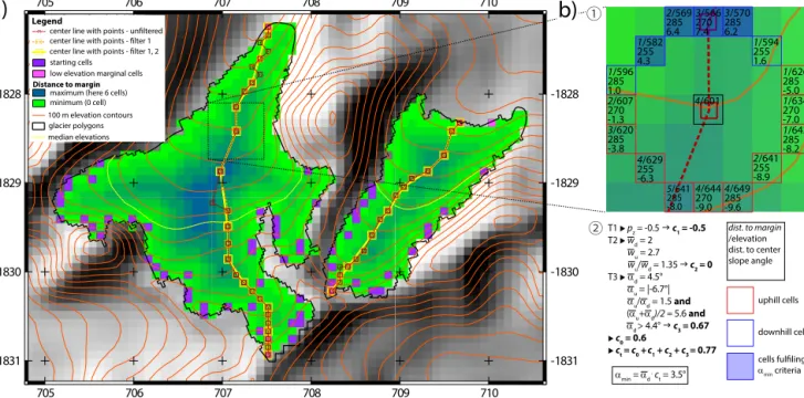
T1 adds weight to slope in the accumulation area of a glacier and gives preference to centrality in the ablation area. The goal is to prioritize centrality on glacier tongues since too much emphasis on slope would make the center lines drift towards the margins as discussed by Schiefer et al. (2008). In the accumulation area, slope receives more weight – oth-erwise center lines maximize centrality at the cost of run-ning diagonally to elevation contours across the surface. The trade-off function expresses the elevation (z) of the current center line point through a dimensionless factor c1: if z is equal to the maximum glacier elevation, then c1=f1; at me-dian elevation c1=0; and c1= −f1at minimum elevation. See the Appendix for a detailed description, a complete list of parameter values and explanations on the numerical example given in Fig. 2b.

T2 emphasizes centrality at locations where a glacier has a constant width and adds weight to slope where the glacier changes width. The function reduces the weight of central-ity where a glacier suddenly widens. This is, for instance, the case at the confluence of two glacier branches. The func-tion is also responsible for a more direct course towards the narrowing glacier termini. A dimensionless factor c2is cal-culated from the ratio of the mean distance to margin of all uphill grid cells (wu) and the mean distance to margin of all downhill grid cells within the search ring wd (see the Ap-pendix for full details).

T3 emphasizes slope in sections where (i) the glacier steepens and (ii) the glacier surface is generally steep. The function achieves a more direct downhill flow in steep glacier sections and a more direct and slope-controlled course where ice masses from an ice cap progress into outlet glacier tongues. Such locations are often associated with a general steepening of the glacier. A dimensionless factor c3is cal-culated based on (i) the ratio of the mean slope αu and αd above and below, respectively, the current elevation of the flow path, and (ii) based on αdalone (see the Appendix for full details).

The basic trade-off factor c0 and the three functions are combined in a nonhierarchical way by ct=P3i=0ci

(cf. Fig. 2b). A minimum slope angle is then calculated ac-cording to αmin=αdct. Finally, from all grid cells fulfilling the αmincondition, the one at maximum distance from the

Figure 1. Flow chart illustrating the concept of center line compu-tation. T1, T2 and T3 refer to the three trade-off functions, F1 and F2 to the two filters. The symbols (1) and (2) relate to the visual-ized example in Fig. 2b. Dotted lines indicate operations related to suggested end points which are only computed for tide-water and lake-terminating glaciers.

-1831 -1831 -1830 -1830 -1829 -1829 -1828 -1828 705 705 706 706 707 707 708 708 709 709 710 710 center line with points - unfiltered

glacier polygons 100 m elevation contours

Legend

Distance to margin

maximum (here 6 cells) minimum (0 cell) center line with points - filter 1 center line with points - filter 1, 2 low elevation marginal cells starting cells median elevations downhill cells uphill cells cells fulfiling αmin criteria

b)

4/601 3/566 270 7.4 2/569 285 6.4 1/582 255 4.3 1/596 285 1.0 2/607 270 -1.3 3/620 285 -3.8 3/570 285 6.2 1/594 255 1.6 1/626 285 -5.0 1/634 270 -7.0 1/642 285 -8.2 2/641 255 -8.9 4/629 255 -6.3 4/644 270 -9.0 4/649 285 -9.6 dist. to margin /elevation dist. to center slope angle 5/641 285 -8.0 T1  pz = -0.5  c1 = -0.5 T2  wd = 2 wu = 2.7 wu/wd = 1.35  c2 = 0 T3  αd = 4.5° αu = |-6.7°| αu/αd = 1.5 and (αu+αd)/2 = 5.6 and αd > 4.4°  c3 = 0.67  c₀ = 0.6  c_t = c₀ +c₁ + c₂ + c₃ = 0.77 αmin = αd . ct = 3.5°

a)

② ①

Figure 2. Concept of the calculation of center lines visualized on the example of two small mountain glaciers of East Greenland. T1, T2 and T3 refer to the three trade-off functions. Note that all calculations are carried out in radians but for the ease of understanding angles are shown in degrees. Coordinates are in kilometers, with polar stereographic projection (EPSG 3413).

glacier margin is chosen as the next center line point. If two or more grid cells are at maximum distance to margin, then the cell with the maximum slope angle is selected as illus-trated in Fig. 2b.

3.4 Suggestion of glacier end points

The autonomous selection of end points (see Sect. 3.2) re-sults in arbitrarily chosen end points on marine- or lake-terminating glaciers with a wide glacier front where even manual definitions of sole glacier end points are debatable. Figure 4 illustrates the issue on the example of two tide-water glaciers. Glacier length could be maximized by measuring at the margins but it appears more logical and consistent to end center lines in the middle of a calving front.

An automated approach is applied to approximate the mid-dle of a calving front and suggest these points as end points. A glacier is assumed to be lake- or marine-terminating when-ever there is a certain number (nc) of grid cells that are (i) located at the glacier margin and (ii) within a certain el-evation threshold (zc) of the lowest grid cell of the glacier (cf. Fig. 4). If these conditions are fulfilled, potential glacier end points are determined by performing a neighborhood analysis where all grid cells fulfilling conditions (i) and (ii) are brought into groups of directly adjacent cells. For each group for which the number of members ng exceeds nc, the geometric center of the location of all group members is calculated. Finally, the group member closest in distance to the geometric center is chosen as a suggested end point.

Since there can be several groups exceeding ncin members, a glacier can have more than one suggested end point.

Calculation of center lines for glaciers with suggested end points is identical to other glaciers with the exception that, as soon as a center line has moved to within a certain distance (De) of a suggested end point, the line is redirected to the end point and the center line is terminated (Fig. 1). Thereby,

De is defined as the maximum distance-to-margin value of all glacier cells located within a radius of C · ng from the potential end point.

3.5 Filtering

Finally two filters are applied to smooth the center lines: – F1: in four iteration steps, points are removed that

de-scribe an angle of less than θ1(θ2in the second to fourth iteration) with their two neighboring points.

– F2: a minimal spacing of Dfmeters between center line points is introduced by deleting points from sections of short spacing between points.

F1 and F2 are applied consecutively. F1 mainly smoothes the center lines in sections where the minimal search radius of one grid cell in each direction is applied. Under these circumstances a center line can find its next point only in eight directions. If the overall direction deviates from these eight angles, the center lines cannot progress in a straight-forward way. Examples are illustrated in Fig. 2a close to the glacier terminus to the west where the unfiltered center

-1831 -1831 -1830 -1830 -1829 -1829 -1828 -1828 705 705 706 706 707 707 708 708 709 709 710 710 glacier polygons 100 m elevation contours Legend Distance to margin

maximum (here 7 cells) minimum (1 cell) longest center line low elevation marginal cells starting cells

median elevations all center lines

Figure 3. All calculated center lines, including the selected longest center lines calculated for two small mountain glaciers of East Greenland. Coordinates as in Fig. 2.

line describes a zigzag pattern. F2 basically reduces the spa-tial resolution of the center lines. The filter is less important on high-quality DEMs as can be seen in Fig. 2a where only marginal changes result. However, the filter is useful in re-moving some of the irregularities in center lines calculated on low-quality DEMs. The filtering introduces a small risk that short sections of a center line run outside of a glacier polygon.

3.6 Calculation of glacier length

For each glacier the same number of center lines is calculated as there are starting cells (Fig. 3). The length of each center line is calculated by summing up the distances between all its individual points, and the length of the longest line is chosen to represent glacier length.

4 Algorithm calibration and evaluation for East Greenland and Alaska

The approach was calibrated on the example of East Green-land by varying the parameters of the trade-off functions and filters until center lines were achieved that fulfill the follow-ing qualitative criteria: center lines should

– cross elevation contours perpendicularly, – flow strictly downhill,

– not cut corners,

– be in the center of the glacier below zmed, – end at the lowest glacier point.

The last two criteria are relevant on typical valley-glacier tongues but can be misleading on certain glacier types such

Figure 4. Concept of “suggested end points” demonstrated on the example of two tide-water glacier of the Geikie Plateau. Coordi-nates as in Fig. 2.

as ice caps without outlet glaciers, ice aprons and cirque-type glaciers. Thus, they are only considered on glaciers where it is assumed that they are in agreement with the characteristics of the actual (imaginary) longest flow line.

4.1 Consideration of inaccuracies in input data

The calibrated algorithm needs to maintain flexibility to deal with inaccuracies in input data. Figure 2a, for instance, exem-plifies a very common problem: the western glacier tongue is shifted relative to the DEM. Thus, flow diagonal to contour lines needs to be tolerated even though the first quality crite-rion is violated. The accumulation areas close to the Green-land Ice Sheet (Fig. 5) show spurious surface undulations. Under such conditions the calculation of reasonable center lines requires a basic ability of “leapfrogging” across smaller undulations at the cost of violating strict downhill flow. The two examples illustrate the aforementioned need for flexi-bility, but the latter must also be limited to avoid erroneous results where input data are of good quality.

The two main compromises for flexibility are the follow-ing: (i) the search radius is always maximized (cf. Sect. 3.2) to reduce the influence of DEM irregularities. Side effects are a reduction of computation time but also possible leapfrog-ging over real surface undulations and a coarse resolution of the center lines where DEM quality would permit a better resolution. (ii) The settings for the trade-off between slope and centrality (Sect. 3.3) are applied in a way that central-ity receives a relatively high weight. For instance the ba-sic parameter c0 is set to 0.6 (Appendix Table A1). In case none of the trade-off functions take effect, this means that the

Figure 5. Calculated longest center lines for the Geikie Plateau, East Greenland. Coordinates as in Fig. 2.

minimum required slope αminis only 60 % of the mean slope angle αdof all downhill cells (cf. Fig. 2). Consequently, only a few of the downhill cells are excluded prior to selecting the cell with maximum distance to margin. Slope thus receives less influence, and center lines maintain a certain flexibility to move laterally.

4.2 Evaluation East Greenland

On average ∼ 22 center lines were calculated per glacier for the East Greenland site, resulting in a total of 88 000 center lines. The longest center line for each glacier of the Geikie Plateau is shown in Fig. 5. Realistic center lines result even

for glacier polygons of highest complexity. The approach performs well on all glacier types, including ice caps and marine-terminating glaciers. Somewhat erratic center lines appear in the wide accumulation areas close to the ice sheet where DEM quality is comparably low (marked with 1 in Fig. 5). Certain center lines do not start at the apparently most distant point of a glacier (marked with 2) because the surface at that location drains into an adjacent glacier.

For the vast majority of glaciers, the center lines end where envisaged, although there are a few locations where the automatic approach suggests erroneous end points. Ex-ample 3 in Fig. 5 illustrates the difficulties in defining repre-sentative end points along complexly shaped calving fronts

of retreating marine-terminating glaciers. The most frequent source of erroneously suggested end points is that DEM and glacier polygons are not contemporaneous. Example 4 shows an erroneous ending due to the complete absence of topog-raphy at the lowermost part of the glacier tongue. While the glacier polygon represents the year 1999 (Rastner et al., 2012), the DEM apparently shows the situation a few years later after a pronounced retreat of the glacier terminus. Non-contemporaneous DEM and glacier polygons are shown in more detail in Fig. 4, where lateral margins are at 0 m a.s.l. for a few kilometers inland, indicating an absence of topog-raphy in the DEM. Indeed, analysis of 2013 satellite imagery shows that the large glacier has retreated by about 8 km since the year 1999. Problems related to non-contemporaneous in-put data mainly occur on marine/lake-terminating glaciers because (i) terminus retreat due to calving can be much faster than the melting of land-terminating glaciers and (ii) calving leaves a perfectly leveled surface behind.

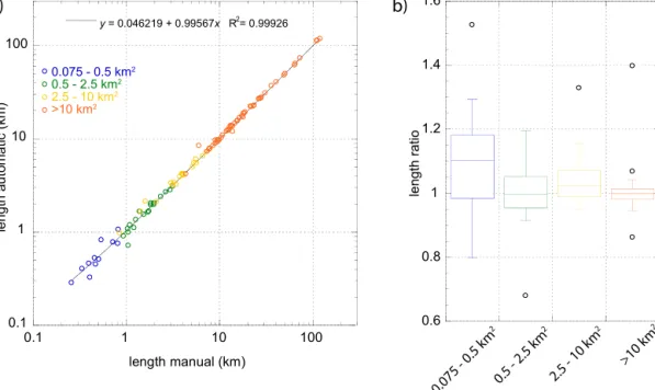
Performance of the algorithm was evaluated by comparing the automatically derived glacier length (La) to manual mea-surements (Lm). To evaluate algorithm performance across most glacier types, 10 size classes were established and, per class, 10 glaciers were randomly selected. The length of the 100 glaciers was then measured manually while automatic center lines were hidden. The averages of automatic and manual glacier length are almost identical (Table 1), while the mean of all glacier specific length ratios Ra/m=La/Lm is 1.02, indicating a small positive bias. The linear regres-sion of Laagainst Lmyields a high correlation (Fig. 6a). De-viations from a perfect agreement (Ra/m=1) are generally small as supported by a root-mean-square deviation (RMSD) of 0.1 (i.e., 10 %, Table 1).

When divided into four glacier size classes, the largest scatter of Ra/m is found for glaciers smaller than 0.5 km2. Deviations are small for larger glaciers and at minimum for glaciers > 10 km2(Fig. 6b). In total there are 14 glaciers (7 of them from the smallest size class) where |Ra/m−1| ex-ceeds 0.1. Analyzing the reasons revealed that six cases can be attributed to erroneous automatic center lines, in one case a manual center line was deemed wrong upon reconsidera-tion and for the remaining seven glaciers both the automatic and the manual center lines appear to be equally valid solu-tions. From the six erroneous center lines, four are from the smallest size class and one results from inconsistencies in the DEM.

4.3 Evaluation Alaska

In the example of the Alaska glacier inventory, automatically derived glacier length was compared to the semi-automatic measurements (Lk) by Kienholz et al. (2014). The compar-ison was done for all 21 720 glaciers exceeding 0.1 km2in area and is summarized in Table 2 and in Fig. 7. By aver-age La is a few percent smaller than Lk, and variability of Ra/k=La/Lkis larger than for East Greenland as indicated

Table 1. Evaluation of algorithm performance in East Greenland

based on 100 randomly selected glaciers. Ra/mdenotes the ratio of

automatic length divided by manual length.

Parameter Value

Average length manually measured 11.48 km

Average length automatically measured 11.46 km

Difference in average length −0.015 km/−0.1 %

Mean of all Ra/m 1.02

Root-mean-square deviation of all Ra/m−1 0.1

Maximum/minimum Ra/m 1.53/0.68

Table 2. Comparison of glacier length calculated by this study and

Kienholz et al. (2014) for 21 720 glaciers. Ra/kdenotes the ratio of

length measured by our approach to length according to Kienholz et al. (2014).

Parameter Value

Average length according 1.99 km

to Kienholz et al. (2014)

Average length this study 1.88 km

Difference in average length −0.11 km/−5.5 %

Mean of all R_a/k 0.93

Root-mean-square deviation of 0.18

all Ra/k−1

Maximum/minimum Ra/k 3.2/0.2

by a higher RMSD and more extreme minimum and maxi-mum values of Ra/k.

Figure 7a indicates that the largest scatter of Ra/kis found for glaciers smaller than 0.5 km2. Figure 7b visualizes the distribution of Ra/kand shows the contributions of the four glacier size classes. In total 64 % of all Ra/k lie within a range of 0.9 to 1.1, 6 % exceed a value of 1.1 and 30 % are below 0.9. These numbers are dominated by the smallest glacier size class, which accounts for 55 % of all investigated glaciers. With increasing glacier size the distribution of Ra/k becomes increasingly centered around Ra/k=1 (Fig. 7b). In the smallest glacier class, 56 % of all Ra/kare within a range of 0.9 to 1.1; the same is the case for 68 % of the glaciers in the second size class, 82 % in the third size class and for 92 % of the glaciers > 10 km2. Values of Ra/k>1.1 are rare for larger glaciers, but there is a relevant fraction of glaciers with Ra/k<0.9 in all size classes (e.g., 36 % of the smallest glaciers, 7 % of the glaciers > 10 km2).

Calculated longest center lines from both approaches are visualized in Fig. 8. The comparison shows a part of the Stikine Icefield, southern Alaska (cf. also Fig. 10 in Kien-holz et al., 2014), where the SRTM elevation model of rel-atively good quality is available. Agreement is high on the larger glaciers, while most of the deviations occur on small ice bodies. The comparison illustrates that often more than

0.1 1 10 100 0.1 1 10 100 le ng th a ut om at ic (k m ) length manual (km)

a)

y = 0.046219 + 0.99567x R2_{= 0.99926} 0.075 - 0.5 km2 0.5 - 2.5 km2 2.5 - 10 km2 >10 km2

b)

length ratio >10 km 2 2.5 - 10 km 2 0.5 - 2.5 km 2 0.075 - 0.5 km 2 0.6 0.8 1 1.2 1.4 1.6

Figure 6. (a) Linear regression of manually (Lm) and automatically (La) measured glacier length for 100 randomly selected glaciers. (b)

Length ratio La/Lmdisplayed for four glacier size classes in box plots. Whiskers refer to 1.5 interquartile range.

0.1 1 10 100 0.1 1 10 100 Le ng th fully automated (k m )

Length semi automated (km)

a)

b)

y = -0.020954 + 0.95277x R2_{= 0.98216} 0.1 - 0.5 km2 0.5 - 2.5 km2 2.5 - 10 km2 >10 km2 0 0.5 1 1.5 2 2.5 3 3.5 4 length ratio 0 2000 4000 6000 8000 10000 0.4 0.6 0.8 1 1.2 1.4 >10 km2 2.5 - 10 km2 0.5 - 2.5 km2 0.1 - 0.5 km2 co un t length ratio _>10 km 2 2.5 - 10 km 2 0.5 - 2.5 km 2 0.1 - 0.5 km 2

Figure 7. (a) Linear regression of glacier length for all Alaskan glaciers determined in an automated way (La, using the approach presented

here) and a semi-automated approach (Lk, Kienholz et al., 2014). (b) Length ratio La/Lkdisplayed for four glacier size classes (cf. Fig. 9 in

Kienholz et al., 2014) in a histogram and box plots. Whiskers in the latter refer to 1.5 interquartile range.

one valid solution exist. There are only a few glaciers where either one or the other approach provides an erroneous result. The comparison for Alaska thus highlights three features: (i) a considerable scatter of Ra/k for small glaciers, (ii) a more general tendency towards Ra/k<1 and (iii) a good agreement of the two approaches provided that DEM data of sufficient quality are available. The deviations on small glaciers are often related to a general ambiguity in defin-ing length. The agreement is best for elongated features with their longer axis pointing downhill. Ambiguities are large for

glacierets located in gently sloping terrain or for polygons of irregular shape. Our approach provides on average a some-what shorter length for small glaciers because calculated cen-ter lines often adhere more strictly to downhill flow, whereas the method developed by Kienholz et al. (2014) tends to cross small polygons more diagonally.

These aforementioned issues are of limited relevance to larger glaciers where Laeither agrees with Lkor underesti-mates actual glacier length due to DEM irregularities. In all cases where Ra/k1, center lines get stopped halfway, and

Figure 8. Direct comparison of longest center lines as calculated in this study and by Kienholz et al. (2014). The figure shows a section of the Stikine Icefield in southern Alaska and the DEM used for the calculation, and also shown in the background is the SRTM v4. Coordinates are in kilometers, UTM zone 8N.

Lais eventually measured from lines that do not represent the entire glacier perimeter. Besides these underestimations there are a few cases where DEM irregularities do not stop a center line but force a detour resulting in an overestimation. Surface slope is an important variable in the automatic approach, and the output thus suffers from the low DEM quality for certain areas of Alaska.

5 Calculated length of all glaciers of the world

By applying the above method to the entire global data set of glacier outlines and DEMs, we evaluated the length and

center lines of all roughly 200 000 glaciers around the globe. Computations are entirely automated, and no glacier, glacier-type or region-specific adjustments were conducted.

Based on the evaluation in East Greenland and Alaska, we estimated typical uncertainties in calculated glacier length. The validation indicated that there is ambiguity in measur-ing the length of small glaciers and that our approach de-pends on DEM quality. As a rule of thumb, uncertainty of glacier length of small glaciers, including any ambiguity, is approximately 20 %. On larger glaciers uncertainty in calcu-lated glacier length depends mainly on DEM quality: uncer-tainty is estimated to be around 2–5 % where the elevation

data are reliable and 5–15 % for regions of lower DEM qual-ity. Furthermore, calculated glacier length can be meaning-less where glacier polygons are erroneous as is the case, for instance, in some areas of northern Asia (cf. Pfeffer et al., 2014, for an in-depth discussion of limitations of the RGI).

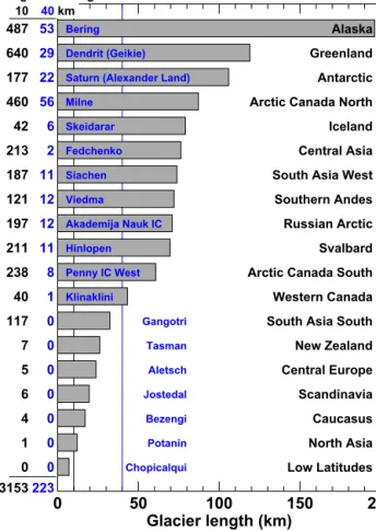
On a worldwide scale, 3153 glaciers outside of the two ice sheets are longer than 10 km, and 223 are longer than 40 km (Fig. 9). The majority of long glaciers are located in the polar regions (Alaska, Arctic Canada, Greenland, Sval-bard, Russian Arctic, Antarctic). However, there are also more than 500 glaciers >10 km in length in high-mountain Asia – Fedchenko and Siachen Glacier are more than 70 km long. Bering Glacier, Alaska/Canada, is the longest glacier in the world (196 km). Glaciers in the periphery of Green-land and Antarctica also reach lengths of more than 100 km (Fig. 9). The maximum glacier length in regions dominated by smaller glaciers (European Alps, Caucasus, New Zealand) is between 10 and 30 km.

Several studies have shown that there is a characteristic scaling between glacier area, volume and length (Bahr et al., 1997; Radic et al., 2008; Lüthi, 2009). In order to analyze the differences in glacier length between individual regions around the globe and to provide a simple mean for estimating glacier length from its area, we derive region-specific scaling relationships of the form

L = k · Aβ, (1)

where L (km) is glacier length along the centerline, A (km2) is glacier area and k (km1−2β) and β (dimensionless) are pa-rameters.

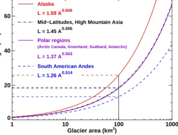
By least-square linear regression for all ∼ 200 000 area– length pairs, k = 1.43 km1−2β and β = 0.556 were deter-mined. Glaciers with areas of 1, 10 or 100 km2thus can be expected to have lengths of 1.4, 5.2 or 18.6 km, respectively. Scaling parameters were also evaluated for four large-scale regions with differing glacier properties: (i) Alaska with the largest valley glaciers, (ii) midlatitude mountain glaciers, (iii) polar regions dominated by ice caps and (iv) the South Amer-ican Andes (Fig. 10). Correlation coefficients in the log–log space were between r2=0.83 and 0.94.

As the differences in glacial morphology and climate are large among the regions, the empirical scaling parame-ters between glacier area and length show some variability (k = [0.92, 1.70], β = [0.467, 0.606]). Expected length for a glacier area of 100 km2 can thus vary between 12 and 26 km (Fig. 10) between the large-scale regions. The longest glaciers for a given area are found in Alaska. This might be explained by the large elevation differences and the chan-neling structure of mountain morphology. Interestingly, mid-latitude glaciers and polar ice caps show very similar area– length scaling parameters, although they greatly differ in shape (Fig. 10). Most likely, different effects of their mor-phology (average slope and width) and climatology (surface mass balance gradients) compensate for each other in terms

0 50 100 150 200 Glacier length (km) Alaska 487 53 Bering Greenland 640 29 Dendrit (Geikie) Antarctic

177 22 Saturn (Alexander Land)

Arctic Canada North

460 56 Milne

Iceland

42 6 Skeidarar

Central Asia

213 2 Fedchenko

South Asia West

187 11 Siachen Southern Andes 121 12 Viedma Russian Arctic 197 12 Akademija Nauk IC Svalbard 211 11 Hinlopen

Arctic Canada South

238 8 Penny IC West

Western Canada

40 1 Klinaklini

South Asia South

117 0 Gangotri New Zealand 7 0 Tasman Central Europe 5 0 Aletsch Scandinavia 6 0 Jostedal Caucasus 4 0 Bezengi North Asia 1 0 Potanin Low Latitudes 0 0 Chopicalqui 3153223

n glaciers longer than

10 40km

Figure 9. Longest glaciers in all regions of the Randolph Glacier Inventory. The glacier name is given in blue (IC: ice cap). The num-ber n of glaciers longer than 10 and 40 km for each region is indi-cated. Note that the length of three glaciers (Milne, Skeidarar and the Akademija Nauk Ice Cap) was measured manually because the automated approach provided incorrect length due to DEM errors.

of the relation between glacier area and length. Glaciers in the South American Andes are found to be shorter for a given area compared to the other regions. The Patagonian Andes are dominated by ice fields at comparably low ele-vations with relatively short outlet glaciers. At low latitudes very steep glaciers prevail that are rarely organized as distinct valley glaciers. Both regions are subject to rather steep bal-ance gradients (Warren and Sugden, 1993; Benn et al., 2005) that limit maximum glacier length.

6 Discussion

6.1 Computation principle

Algorithm development was guided by the idea to mimic glacier flow with simple and computationally efficient algo-rithms using the full information available in a DEM. The first condition of maximizing downhill slope imitates grav-itational pull, while the condition of centrality emulates the

1 10 100 1000 Glacier area (km2₎ 0 20 40 60 Glacier length (km) Alaska L = 1.59 A 0.606

Mid−Latitudes, High Mountain Asia L = 1.45 A 0.555

Polar regions

(Arctic Canada, Greenland, Svalbard, Antarctic)

L = 1.37 A 0.563 South American Andes L = 1.26 A 0.514

Figure 10. Scaling relationships between glacier area A and length

Lderived for four subsets of glacier regions. The scaling parameters

are given, and a reading example for a glacier with A = 100 km2is

shown.

guiding effect of the surrounding ice masses. Calculated flow trajectories are not to be taken as actual flow lines because glacier flow is a three-dimensional phenomenon and can-not be derived from surface information alone. Furthermore, glacier flow lines adjoin on glacier tongues in parallel flow, while our trajectories unite in one central line. Then again our approach does not necessarily generate center lines in a strict sense. Adherence to the glacier center can be flexibly varied across the glacier perimeter. With the settings applied here, centrality is less rigid than in previously published methods (Le Bris and Paul, 2013; Kienholz et al., 2014).

We have presented one possibility of implementing the ba-sic conditions and designing trade-off functions; alternatives to improve accuracy and efficiency certainly exist. In partic-ular, this concerns the trade-off between surface slope and centrality, where alternative designs should be explored. One might also imagine involving additional conditions, such as the direct inclusion of observed glacier flow fields.

The approach is computationally efficient; 41 000 km2of glaciers at 90 m spatial resolution (East Greenland) are calcu-lated within 15–20 min on an ordinary laptop computer. This efficiency is used to apply a “brute-force” method of start point sampling. The point density is simply set high enough so that every glacier branch receives several starting points. The probability that the most distant point is among the sam-pled ones is high, independent of whether the point is located on a summit, a pass or elsewhere. A geometric order of cen-ter lines can be established using the method by Kienholz et al. (2014) but is computationally more demanding due to the large number of center lines.

Our approach is applied in an automated manner but is programmed to allow for similar possibilities of manual in-tervention as illustrated by Kienholz et al. (2014). For the

worldwide calculation none of these options was used how-ever.

6.2 Algorithm performance

Evaluation of the algorithm indicates good performance for the East Greenland test site, while the comparison for Alaska shows stronger deviations between the methods.

The major reason for the success of the East Greenland calculation is seen in the quality of the GIMP DEM, which allows for accurately calculated center lines. Basic character-istics of topography are well represented in the DEM, and the artifacts consisting of spurious surface undulations are small enough not to interfere with the calculations. A further rea-son for the good agreement is that manual drawing of center lines strongly relied on surface topography, and only obvi-ously erroneous topographic features were ignored. The fact that the algorithm was calibrated for the region is likely of limited relevance because the area comprises virtually every possible glacier type, including very complex glacier shapes. Laborious manual measurement allowed us to measure only 100 glaciers randomly picked from 10 predefined size classes. Thus, small glaciers are underrepresented compared to the full set of East Greenland glaciers. Furthermore, the average glacier area in East Greenland is larger by almost a factor of 3 compared to Alaska (11.0 km2vs. 4.0 km2). The influence of ambiguities and issues related to small glaciers is thus underrepresented in the evaluation for Greenland. Nev-ertheless, a visual review of most Greenland center lines (cf. Fig. 5) confirms the good performance that resulted in the 100 glacier sample.

In the Alaska comparison, a good correlation is found where DEM quality is comparable to the East Greenland GIMP DEM, but strong deviations in measured glacier length occur in low-quality DEMs. A qualitative assessment with focus on the two DEMs most frequently used in the global calculation suggests that performance is high in the SRTM DEM but worse in the ASTER GDEM v2. In the latter, cen-ter lines are sometimes cen-terminated midway, where DEM er-rors suggest that a glacier tongue flows uphill over a distance longer than the applied search radius. The approach by Kien-holz et al. (2014) mostly maintains the ability to continue center lines because the method does not suppress uphill flow for the major (lower) part of a glacier. Low-quality DEMs are also the main reason for different starting points cho-sen by the two approaches. Basically our high sampling den-sity would guarantee that, nearly everywhere, starting points are picked in close proximity to the points chosen by Kien-holz et al. (2014). However, DEM irregularities might block progress towards the glacier tongue and force center lines to end too early. Other lines starting lower down might become longer and be eventually chosen to represent total glacier length.

In the example of Alaska, we compared our automated method to the measurements of Kienholz et al. (2014) that

involved a considerable number of manual interventions. Only a rough estimate can be provided on how our method would perform if a similar number of manual corrections were to be applied. We assume that DEM-related issues could be alleviated only marginally, but manual definitions of glacier end points would be of considerable benefit on piedmont-type glacier tongues where the automatic selection of end points often produces unsatisfying results.

The difficulties with low-quality DEM data are rooted in the strong dependence on surface slope. Relying on the lat-ter, however, is an advantage for certain glacier types, and also more generally when calculating center lines on high-quality DEMs. Considering surface slope is of particular im-portance on wide ice aprons, asymmetric glacier shapes and ice caps, and where broad accumulation areas narrow into tongues of outlet glaciers. When relying strongly on central-ity, center lines can run almost parallel to elevation contours. For such specific glacier types, and more generally wherever high-quality DEMs exist, our approach leads to stricter con-trol of unphysical lateral flow.

Our approach has no strong dependency on catchment de-lineations due to the strong involvement of surface slope. If the trade-off between centrality and slope is re-calibrated accordingly, approximate flow lines can be calculated for glacier complexes or ice caps without any catchment de-lineations. The importance of centrality in the approach by Kienholz et al. (2014) leads to a stronger dependency on ac-curate catchment delineations, which are only possible when a certain level of DEM quality is given. Thus, both ap-proaches depend on DEM quality, albeit to a varying degree and at different stages of the calculations.

6.3 Worldwide glacier length

Glacier length is an important yet missing parameter in global glacier inventories (Paul et al., 2009). The GLIMS (Global Land Ice Measurements from Space) Glacier Database, for instance, stores center lines for glaciers, and currently contains center lines for about 2300 glaciers. Here we provide a first globally complete assessment of the length of all ∼ 200 000 individual glaciers around the globe. Based on our data we investigate the relationship of glacier length and glacier area and calculate global and regional scaling laws. Differences between the regions appear to be related to regional characteristics of topography and mass balance distribution. Due to large variability in glacier shapes, the scaling laws allow only a rough estimate of the length of in-dividual glaciers. A particularly wide spread exists among small glaciers because of ambiguities in defining their length (cf. Le Bris and Paul, 2013), but given their small size the application of scaling laws involves only limited absolute er-rors.

For reasons discussed above, our global data set of glacier length is subject to regionally varying quality. Low uncer-tainties can be expected where the SRTM or better-quality DEM data were used, i.e., between latitudes of 60◦N and 55◦S, as well as for the Greenland (GIMP DEM) and the Antarctic (RAMP DEM) periphery. Limited accuracy is achieved for most Arctic regions where the ASTER GDEM v2 had to be used, in particular for Arctic Canada and the Russian Arctic. Glacier length data from areas with RGI quality limitations should also be used with care.

7 Conclusions

We have presented a grid-based and automated algorithm to calculate glacier center lines. Our method is based on the two conditions of maximizing surface slope and distance to the glacier margin. A set of three trade-off functions ana-lyzes the local morphometry of the glacier and, depending on the latter, flexibly controls the weight of the two basic conditions. The approach was developed using East Green-land as a test area, evaluated for East GreenGreen-land as well as for Alaska and then applied to obtain the first global assessment of glacier length. By calculating glacier length for each of the

∼200 000 glaciers in the RGI, we add an important and pre-viously unavailable parameter to global glacier inventories.

Our scaling laws and the differences in scaling factors among regions can be applied and investigated in the frame-work of conceptual glacier models. Global glacier length data could potentially be used to assess changes in length for different regions or glacier types. The actual center lines might be beneficial to flow-line modeling approaches.

Our approach calculates center lines by mimicking glacier flow and is computationally efficient and automated. Thus, three of the initially stated four conditions are met. While ac-curate center lines result when using high-quality DEM data, further research is needed to reduce the method’s sensitivity to DEM inaccuracies. With the upcoming TanDEM-X data in view (e.g., Martone et al., 2013), however, we believe that our basic concept is well suited for future use. Once these precise worldwide terrain data are available, we will aim at providing an updated high-quality data set of global glacier length.

Appendix A

A1 Trade-off functions

In the following the three trade-off functions are explained in full detail. Figure 2b shows a numerical example of the use of the trade-off functions.

T1: the first trade-off function (i) decreases the weight of centrality in the accumulation area where glacier cross sec-tions are usually concave and (ii) increases the impact of centrality in the often convexly shaped ablation area. The trade-off function firstly expresses the current elevation z as zp=(z − zmed)/(zmax−zmed) if z > zmed and as zp= (z − zmed)/(zmed−zmin)if z ≤ zmed; zmaxand zminare max-imum and minmax-imum glacier elevation, respectively. Hence 0 < zp≤1 if z falls into the accumulation area and −1 ≤ zp≤0 if z falls into the ablation area. The basic idea is to use a c1value for the ablation zone and another value for the ablation zone. An arcus tangent function is applied to avoid a stepwise transition at zmed. The smoother transition also ac-counts for the fact that the elevation of the transition from a concave to a convex glacier cross section can vary across a glacier and is not strictly linked to zmed. From zp a factor c1is calculated according to c1=f1·atan(100 zp)(π/2). In

the example given in Fig. 2b, c1is computed to be −0.494 ≈ −0.5.

T2: the trade-off function firstly calculates the mean dis-tance to margin of all uphill grid cells (wu) and the mean dis-tance to margin of all downhill grid cells (wd). Only grid cells are considered that are located on the current search ring. Subsequently, it is checked whether |wu/wd−1| > t2, where t2is a threshold value. If the condition is fulfilled, then a fac-tor c2is calculated according to c2=f2(|wu/wd−1|). The calculation of c2 depends on relative glacier width, which guarantees a similar behavior on wide and narrow glaciers. The factors t2 and f2 were varied until satisfactory center lines resulted in (i) confluence areas and (ii) locations of pronounced glacier narrowing. Since t2 is set to 0.35 (Ta-ble A1), the example in Fig. 2b does not fulfill the condition

|wu/wd−1| > t2and c2remains zero.

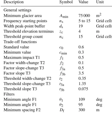
Table A1. Model parameters resulting from the East Greenland cali-bration and applied for the worldwide calculations. Parameters used

for Alaska are identical apart from Amin=100 000 m2.

Description Symbol Value Unit

General settings

Minimum glacier area Amin 75 000 m2

Frequency starting points ns 5 to 15 Grid cells

Width peak-point buffer ds 19 Grid cells

Threshold elevation terminus zc 4 m

Threshold group count nc 15 Grid cells

Trade-off functions

Standard value c0 0.6

Minimum value cmin 0.3

Maximum impact T1 f1 0.5 Factor width-change T2 f2 0.1 Factor slope-change T3 f3a 0.5 Factor slope T3 f3b 3.5 Threshold width-change T2 t2 0.35 Threshold slope-change T3 t3a 1.35 Threshold slope T3 t3b 0.075 Filters

Minimum angle F1 θ1 109 deg

Minimum angle F1 θ2 95 deg

Minimum spacing F2 Df 300 m

T3: the trade-off function firstly calculates the mean slope angle above (αu) and below (αd) the current elevation of the flow path by averaging slope to all uphill and downhill grid cells. As with T2, only cells located on the current search ring are considered. If the ratio αu/αd exceeds a certain thresh-old t3a and the mean slope (αu+αd)/2 is within a range of 0.02 to 0.1, then a factor c3 is calculated according to c3=f3a(αu+αd)/2. If (αu+αd)/2 > 0.1, then c3=f3a·0.1. The factors t3a and f3a and the range of 0.02 to 0.1 were calibrated while observing the center line behavior on lo-cations where glaciers suddenly steepen. The latter is fre-quently the case at the starting zone of outlet glaciers of ice caps. In addition αdis checked, and if it exceeds a thresh-old t3b, then c3=c3+αd·f3b. This second condition was in-troduced to specifically reduce the influence of centrality on steep glaciers. In the example of Fig. 2b all three conditions are met: αu/αd> t3a, 0.02 ≤ (αu+αd)/2 ≤ 0.1 and αd> t3b. Thus c3is calculated to be 0.67.

A2 Parameter settings

The chosen settings for all parameters of the algorithm are listed in Table A1.

Acknowledgements. We are grateful to C. Kienholz, University of

Alaska, Fairbanks, for providing the Alaska glacier length, center line and DEM data. The reviews by B. Raup and C. Kienholz helped to clearly improve the manuscript. This publication is contribution number 40 of the Nordic Centre of Excellence SVALI, “Stability and Variations of Arctic Land Ice”, funded by the Nordic Top-level Research Initiative (TRI).

Edited by: A. Kääb

References

Bahr, D. B., Meier, M. F., and Peckham, S. D.: The physical basis of glacier volume-area scaling, J. Geophys. Res., 102, 20355– 20362, 1997.

Benn, D. I., Owen, L. A., Osmaston, H. A., Seltzer, G. O., Porter, S. C., and Mark, B.: Reconstruction of equilibrium-line altitudes for tropical and sub-tropical glaciers, Quarternary Int., 138, 8–21, 2005.

Braithwaite, R. and Raper, S.: Estimating equilibrium-line altitude (ELA) from glacier inventory data, Ann. Glaciol., 50, 127–132, 2009.

Cogley, J. G.: A more complete version of the World Glacier Inven-tory, Ann. Glaciol., 50, 32–38, 2009.

Hoelzle, M., Haeberli, W., Dischl, M., and Peschke, W.: Secular glacier mass balances derived from cumulative glacier length changes, Global Planet. Change, 36, 295–306, 2003.

Howat, I. M., Negrete, A., and Smith, B. E.: The Greenland Ice Mapping Project (GIMP) land classification and surface eleva-tion data sets, The Cryosphere, 8, 1509–1518, doi:10.5194/tc-8-1509-2014, 2014.

Huss, M. and Farinotti, D.: Distributed ice thickness and volume of all glaciers around the globe, J. Geophys. Res., 117, F04010, doi:10.1029/2012JF002523, 2012.

Jarvis, J., Reuter, H., Nelson, A., and Guevara, E.: Hole-filled SRTM for the Globe, CGIAR-CSI SRTM 90 m Database, Ver-sion 4, available at: http://srtm.csi.cgiar.org/ (last access: Decem-ber 2013), 2008.

Kienholz, C., Rich, J. L., Arendt, A. A., and Hock, R.: A new method for deriving glacier centerlines applied to glaciers in Alaska and northwest Canada, The Cryosphere, 8, 503–519, doi:10.5194/tc-8-503-2014, 2014.

Le Bris, R. and Paul, F.: An automatic method to create flow lines for determination of glacier length: a pilot study with Alaskan glaciers, Comput. Geosci., 52, 234–245, 2013.

Leclercq, P. W., Weidick, A., Paul, F., Bolch, T., Citterio, M., and Oerlemans, J.: Brief communication “Historical glacier length changes in West Greenland”, The Cryosphere, 6, 1339–1343, doi:10.5194/tc-6-1339-2012, 2012.

Leclercq, P. W., Oerlemans, J., Basagic, H. J., Bushueva, I., Cook, A. J., and Le Bris, R.: A data set of worldwide glacier length fluctuations, The Cryosphere, 8, 659–672, doi:10.5194/tc-8-659-2014, 2014.

Liu, H., Jezek, K., Li, B., and Zhao, Z.: Radarsat Antarctic Map-ping Project Digital Elevation Model Version 2, National Snow and Ice Data Center, Digital media 01/2001, Boulder, Colorado, USA, 2001.

Lüthi, M. P.: Transient response of idealized glaciers to climate vari-ations, J. Glaciol., 55, 918–930, 2009.

Martone, M., Rizzoli, P., Bräutigam, B., and Krieger, G.: First 2 years of TanDEM-X mission: interferometric performance overview, Radio Sci., 48, 617–627, doi:10.1002/2012RS005095, 2013.

Nussbaumer, S. U., Zumbühl, H. J., and Steiner, D.: Fluctuations of the Mer de Glace (Mont Blanc area, France) AD 1500–2050: an interdisciplinary approach using new historical data and neural network simulations, Zeitschrift für Gletscherkunde und Glazial-geologie, 40, 1–175, 2007.

Oerlemans, J.: Extracting a climate signal from 169 glacier records, Science, 308, 675–677, 2005.

Paul, F., Barry, R., Cogley, J., Frey, H., Haeberli, W., Ohmura, A., Ommanney, C., Raup, B., Rivera, A., and Zemp, M.: Recommendations for the compilation of glacier in-ventory data from digital sources, Ann. Glaciol., 50, 119–126, doi:10.3189/172756410790595778, 2009.

Pfeffer, W. T., Arendt, A. A., Bliss, A., Bolch, T., Cogley, J. G., Gardner, A. S., Hagen, J., O., Hock, R., Kaser, G., Kienholz, C., Miles, E. S., Moholdt, G., Mölg, N., Paul, F., Radic, V., Rastner, P., Raup, B. H., Rich, J., Sharp, M. J., and the Ran-dolph Consortium: The RanRan-dolph Glacier Inventory: a glob-ally complete inventory of glaciers, J. Glaciol., 60, 537–552, doi:10.3189/2014JoG13J176, 2014.

Planchon, O. and Darboux, F.: A fast, simple and versatile algorithm to fill the depressions of digital elevation models, Catena, 46, 159–176, 2001.

Radic, V., Hock, R., and Oerlemans, J.: Analysis of scaling meth-ods in deriving future volume evolutions of valley glaciers, J. Glaciol., 54, 601–612, 2008.

Rastner, P., Bolch, T., Mölg, N., Machguth, H., Le Bris, R., and Paul, F.: The first complete inventory of the local glaciers and ice caps on Greenland, The Cryosphere, 6, 1483–1495, doi:10.5194/tc-6-1483-2012, 2012.

Schiefer, E., Menounos, B., and Wheate, R.: An inventory and morphometric analysis of British Columbia glaciers, Canada, J. Glaciol., 54, 551–560, 2008.

Tachikawa, T., Kaku, M., Iwasaki, A., Gesch, D., Oimoen, M., Zhang, Z., Danielson, J., Krieger, T., Curtis, B., Haase, J., Abrams, M., Crippen, R., and Carabajal, C.: ASTER Global Dig-ital Elevation Model Version 2 – Summary of Validation Results., Tech. rep., NASA Land Processes Distributed Active Archive Center and the Joint Japan-US ASTER Science Team, 2011. Warren, C. R. and Sugden, D. E.: The Patagonian icefields: a