C
ONNECTINGp-
GONAL LOCI IN THE COMPACTIFICATION OF MODULI SPACEAntonio F. Costa, Milagros Izquierdo, Hugo Parlier†
Abstract: Consider the moduli space Mg of Riemann surfaces of genus g ≥ 2 and its Deligne-Munford compactificationMg. We are interested in the branch locusBgfor g >2,
i.e., the subset ofMg consisting of surfaces with automorphisms. It is well-known that the set of hyperelliptic surfaces (the hyperelliptic locus) is connected inMg but the set
of (cyclic) trigonal surfaces is not. By contrast, we show that for g ≥5 the set of (cyclic) trigonal surfaces is connected inMg. To do so we exhibit an explicit nodal surface that lies in the completion of every equisymmetric set of 3-gonal Riemann surfaces. For p>3 the connectivity of the p-gonal loci becomes more involved. We show that for p ≥11 prime and genus g = p−1 there are one-dimensional strata of cyclic p-gonal surfaces that are completely isolated in the completionBgof the branch locus inMg.
1. INTRODUCTION
For g ≥ 2, moduli space Mg is the set of conformal structures that one can put on a closed surface of genus g. As a set it admits many structures and can naturally be given an orbifold structure where the orbifold points correspond exactly to those surfaces with conformal automorphisms. One way of seeing this structure is by seeing moduli space through the eyes of Teichm ¨uller theory. Teichm ¨uller space is the deformation space of marked conformal structures and is diffeomorphic toR6g−6 =C3g−3. From this, moduli space can be seen as the quotient of Teichm ¨uller space by the mapping class group, i.e, the group of homeomorphisms of the surface up to isotopy, which naturally acts on Teichm ¨uller space via the marking and as such the mapping class group is the orbifold fundamental group of the moduli space. The orbifold points of a moduli space appear when the surfaces in question have self-isometries and the groups of self-isometries correspond to the finite subgroups of the mapping class group. (In the genus 2 case this is not strictly correct because †All authors partially supported by Ministerio de Ciencia e Innovacion grant number MTM2011-23092 and third author supported by Swiss National Science Foundation grant number PP00P2 128557
2010 Mathematics Subject Classification: Primary: 14H15. Secondary: 30F10, 30F60.
Key words and phrases: hyperbolic surfaces, isometries of surfaces, branch locus of moduli space
every surface is hyperelliptic, so orbifold points correspond to surfaces with additional self-isometries.) An important step in understanding the topology, and in general, the structures that moduli space carries, is in understanding these particular points. The set of these points is generally called the branch locus and is denotedBg.
With the exception of some low genus cases, Bg is disconnected [BCI1] and displays
all sorts of phenomena including having isolated points [K]. The points of Bg can be organized in strata corresponding to surfaces with the same isometry group and the same topological action of the isometry groups on the surfaces [B] . The closure of each strata is an equisymmetric set. Each equisymmetric set is connected [Na], theorem 6.1 (see also [MS]) and consists of surfaces with isometry group containing a given finite group with a fixed topological action.
Furthermore, the set of Riemann surfaces that are Galois coverings of the Riemann sphere with a fixed Galois group is a union of equisymmetric sets and corresponds to the loci of algebraic curves that admit a determined algebraic expression. The most simple case is the (cyclic) p-gonal locus which is the set of points inMgcorresponding to Riemann surfaces
that are p-fold cyclic coverings of the Riemann sphere. These are called cyclic p-gonal Riemann surfaces and in the case where p is prime, having a p-gonal Galois covering is equivalent to being cyclic p-gonal. From the algebraic curve viewpoint these surfaces are those corresponding to an equation of type
yp= Q(x)
where Q is a polynomial. Note that if the p-gonal locus is connected it is possible to continuously deform any cyclic p-gonal curve to other one keeping the p-gonality along the deformation (see [SeSo]).
The first result in this direction was to show the connectivity of the hyperelliptic locus [Na] , i.e., the set of surfaces invariant by a conformal involution with quotient a sphere. Note that as a subset of Teichm ¨uller space it is disconnected. From the algebraic curve viewpoint these surfaces are those corresponding to an equation of type
y2 =Q(x)
where Q is a polynomial. In contrast, cyclic trigonal surfaces, i.e., surfaces with an auto-morphism of order 3 whose quotient is a sphere, are known to form disconnected loci ofBg
(see [BSS]). These surfaces this time correspond to surfaces with an equation of type y3 =Q(x).
As p increases, the behaviors of the corresponding p−gonal loci become more exotic. For instance one can even find one (complex) dimensional equisymmetric sets consisting of p-gonal surfaces and completely isolated insideBg, the first example of this being equisym-metic sets of 11-gonal surfaces in genus 10 [CI2]. More generally, the connectivity of the branch locus for different types of group actions and properties of equisymmetric sets have been well studied and we refer the interested reader to [BCIP], [BCI1],[BCI2],[BCI3],[BI], [BSS], [CI3], [Se].
In this paper we turn our attention to the Deligne-Mumford compacitification Mg of moduli space which is obtained by adding so-called nodal surfaces. From the hyperbolic viewpoint, these are surfaces where a geodesic multicurve has been pinched to length 0. From the viewpoint of algebraic curves, deformations correspond to variation in the coefficients or roots of the polynomials and these nodal surfaces correspond to algebraic curves with singularities.
Our first point of focus is on the connectivity of the cyclic trigonal locus described above but this time inMg. Our main result is the following.
Theorem 1.1. For g ≥ 5, there is an explicit nodal surface that lies in completion of all the equisymmetric sets in the 3-gonal locus. In particular, the set of (cyclic) trigonal surfaces is connected inMg.
Because there is a single surface that connects all of the equisymmetric sets, from the equation viewpoint this implies that any two cyclic trigonal equations can be deformed continuously from one to the other, where one allows the passage through at most one nodal surface.
In light of the above one might expect that this type of phenomena continues to occur for higher order cyclic p-gonal surfaces but in fact this fails in general. To show this we restrict our attention to 1-dimensional cyclic p-gonal strata in genus g= p−1 for p prime. The connectivity already fails for 4−gonal locus but this is less telling as the non-primality of 4 induces different phenomena.
We show that already for p =5, one connected component of the cyclic 5-gonal locus in genus 4 continues to be disconnected at the boundary. We generalize this to higher genus to obtain the following.
Theorem 1.2. For p ≥ 11 prime, there are completely isolated one-dimensional strata inBp−1
corresponding to cyclic p-gonal surfaces.
any isolated one dimensional strata inMglet alone its completion. Organization.
The article is organized as follows. We begin with a section of preliminaries which includes well known results and certain basic lemmas we will need in the sequel. We then prove the connectivity of cyclic trigonal surfaces in the compactification. The last section deals with cyclic p−gonal surfaces in genus p−1.
Acknowledgements.
The authors are grateful to Jeff Achter for pointing out the relationship between Theorem1.1
and [AP, Prop. 2.11]. The first and third authors are grateful to the University of Link ¨oping for hosting them for a stay during which substantial progress was made on this work.
2. PRELIMINARIES
Let f : S →C be an l-fold branched covering and letˆ {b1, . . . , br}be the set of branched
points. Let o be a point in ˆC\ {b1, . . . , br}and assume f−1(o) = {o1, . . . , ol}.
We define the monodromy ωf of f as a map
ωf : π1(Cˆ \ {b1, . . . , br}, o) →Σl = P {1, . . . , l}
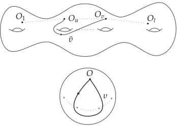
as follows. Let y= [ν] ∈π1(Cˆ \ {b1, . . . , br}, o), where ν is a loop based in o. Now ωf(y)is
a permutation on{1, . . . , l}which takes u∈ {1, . . . , l}to v∈ {1, . . . , l}(i.e. ωf(y)(u) =v)
if the lift ˜ν of ν with origin in oufinishes in ov.
O1 Ou Ov Ol
O ˜υ
υ
Figure 1: An illustration of ˜υ for a simple loop υ
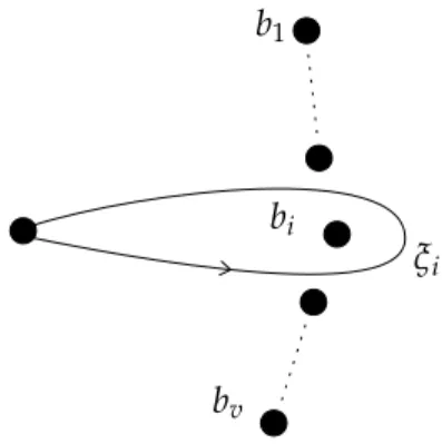
simple loop ξibased at o that bounds a disk which contains biand none of the other branch points. b1 bi bv ξi
Figure 2: The loop ξi corresponding to the meridian xi
Meridians will be useful in the sequel as they are natural generators of the fundamental group π1(Cˆ \ {b1, . . . , br}, o)and monodromy representations are entirely determined by
which permutation one associates to these elements. Specifically a set x1, . . . , xr is said
to be a canonical set of generators of π1(Cˆ \ {b1, . . . , br}, o)if the xiare all meridians and
π1(Cˆ \ {b1, . . . , br}, o)admits the following group presentation:
< x1, . . . , xr|x1. . . xr=1>.
One fact we will use regularly is that there is a lower bound on the length of closed geodesics that pass through fixed points of automorphisms provided the automorphism has order
>2. More specifically we have:
Lemma 2.1. Let S be a hyperbolic surface and h an automorphism of S of order d>2. Then there exists a constant Cd > 0 such that every closed geodesic γ that passes through at least one fixed
point of h satisfies
`(γ) >Cd.
Furthermore one can take Cd ≥2 arccoshsin12π d
.
Proof. Consider O := S/ < h >is an orbifold and γ projects to a closed geodesic γ0 on S/ <h>which passes through an orbifold point of order d and satisfies
Now by the collar theorem on orbifold surfaces [DP], the length of any geodesic segment that passes through the collar is at least
arccosh 1 sin2πd which gives the lower bound on the length of γ.
A slightly more general lemma is indeed true but this is sufficient for our purposes.
3. THE TOPOLOGY OF THE BRANCH LOCUS OF CYCLIC TRIGONAL SURFACES Definition 3.1. A trigonal surface is a Riemann surface S such that there exists a 3-fold covering from S to the Riemann sphere ˆC. The morphism f : S→C is called the trigonalˆ
morphism. If the covering is regular, the surface is said to be cyclic trigonal. One can express that a surface is 3-gonal in terms of the monodromy [ST]:
Proposition 3.2. f : S→C is cyclic trigonal if and only if the monodromy representation is asˆ
follows:
ωf : π1(Cˆ \ {b1, . . . , br}, o) → Σ3
xi 7→ (1, 2, 3)or(1, 3, 2)
We’re interested in the case where are surfaces that can be endowed with a hyperbolic metric, thus we suppose that the genus g of the surfaces is≥ 2. In this case, the surfaces admit a characterization in terms of Fuchsian groups.
Proposition 3.3. S is cyclic trigonal if and only if there exists a Fuchsian groupΦ of signature (0,
r
[3, . . . , 3])and an epimorphism θ :Φ→C3such that S=H/ ker(θ)and such that θ(x) 6=1
for each x elliptic inΦ.
Consider x1, . . . , xr a canonical set of generators of π1(Cˆ \ {b1, . . . , br}, o), i.e. π1(Cˆ \
{b1, . . . , br}, o)admits the following group presentation:
< x1, . . . , xr|x1. . . xr=1>.
Now the permutation t := (1, 2, 3) generates C3 as subgroup of Σl = P {1, 2, 3} and
ωf(xi) =t or t−1for each i. We denote by m+the number of generators sent to t and by m−the number of generators sent to t−1(by ω).
The quantities m+and m−satisfy the following equalities:
m++m−=r= g+2 (1)
and
m++2m− ≡0 mod 3. (2)
The first equality is just by definition and the second comes from the equality in C3given
by
ω(x1. . . xr) =idC3
from which it follows that
tm++2m− =id C3.
The following proposition due to Nielsen says that m+determines the morphisms topolog-ically [Ni].
Proposition 3.4. Two cyclic trigonal morphisms f1 : S1 →C and fˆ 2 : S2→C are topologicallyˆ
equivalent if and only if m+(S1, f1) =m+(S2, f2).
LetMm+=k
g be the set of points inMgcorresponding to cyclic trigonal surfaces(S, f)with
topological type given by m+(S, f) =k.
Proposition 3.5(Consequence of [Na] and [G]). For all k,Mm+=k
g is connected and if k6=k0
Mm+=k
g ∩ Mm+=k 0
g =∅.
We can now state our first theorem. Theorem 3.6. Let I= {k| Mm+=k g 6=∅}. Then \ k∈I Mgm+=k 6=∅.
Note that this theorem can be also be deduced using computations in [AP, Prop. 2.11], although here we shall give a complete proof in terms of hyperbolic structures on Riemann surfaces.
To prove the theorem we shall show the existence of an explicit nodal surface that belongs to the completion of each of the strata. To construct this surface we need the following lemma which guarantees the unicity of specific punctured surfaces which will serve as building blocks of our nodal surface.
Lemma 3.7. Up to isometry, there are unique (and distinct) hyperbolic complete finite area surfaces that satisfy the following properties:
1. Q is a once punctured torus with an isometry of order 3,
2. α is a twice punctured torus with an automorphism of order 3 with 2 fixed points, 3. X is a 4 times punctured sphere with one automorphism of order 3 with one fixed point. Proof. Case1is just the well known fact that the so-called modular torus is the unique punctured torus with an automorphism of order 3. The conformal automorphism of order 3 has 3 fixed points, just choose one of them to remove and obtain a cusp (note there are isometries in that torus interchanging the three fixed points).
The surface α is obtained by considering the unique hyperbolic torus with two cusps in the conformal class of the modular torus with two of the fixed points removed and which become cusps.
Now consider a pair of pants with three cusps as boundary. It clearly has an automorphism of order three which rotates the cusps and has 2 fixed points. X is the unique hyperbolic surface one obtains by removing one of the fixed points to obtain a cusp. Uniqueness is again guaranteed by the uniqueness of the conformal class of a thrice punctured pair of pants.
Proof of Theorem3.6. We begin by endowing S with a hyperbolic metric. Then S admits an automorphism h of order 3 such that S/<h>is a hyperbolic orbifold of genus 0.
The construction of our nodal surface will be algorithmic and we begin by considering a specific pants decomposition of S/<h>where the boundaries of pants are either simple closed geodesics or branched points.
Let B be the set of branched points{b1, . . . , br}. Let ωf : π1(Cˆ \ {b1, . . . , br}, o) →Σ3be the
monodromy of f : S→S/ <h>=C.ˆ
Now B= B+∪B−where B+(resp. B−) is the subset of B consisting of points bisuch that
ωf(xi) =t (resp. ωf(xi) =t−1).
We are going to arrange a maximum number of points of B into triples where each triple lies in a Bi. Specifically let T := b#B3+c + b
#B−
3 c. And set{bk1, b2k, b3k}Tk=1so that
{bk1, bk2, bk3} ⊂Bi
Initial step
We now construct a first pair of pants. Consider disjoint simple closed geodesics γ11, γ12 such that γ11, b11, b12and γ11, γ12, b13are the boundaries of embedded pairs of pants. (There are infinitely many choices for such curves.)
b11 b21 b13
γ11 γ12
Figure 3: The curves γ11and γ21 General step
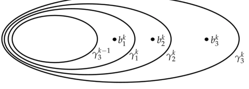
Now for k ∈ {2, . . . , T}we construct simple closed geodesics γk1, γ2k, γ3k, belonging to the portion of S/< h>from which we have removed the pants constructed previously, with the following properties:
γ3k−1, γk1, b1k; γ1k, γk2, b2k
and
γ2k, γk3, b3k
are the boundary curves of embedded pairs of pants. (Again there are many choices for these curves.)
b1k bk2 bk3
γ3k−1 γk1 γk2 γk
3
Figure 4: The general step
Recall that m+ and m−satisfy equations1and 2. As such there are 3 cases to consider depending on the number of branch points that do not belong to the pants we have
constructed. Following equation2, we have
m+ ≡m− mod 3
and thus the number of points is either 0, 2 or 4, and the number of remaining points from B−is the same as the number from B+.
- If there are none, then note that the final 2 curves of our pants decomposition were in fact trivial.
- Suppose we have 1 in both B+ and B− (say b and ˜b: then the set of curves we have constructed form a full pants decomposition of S/ < h > and the final pair of pants is
γ3T, b, ˜b.
- Suppose we have 2 in both B+and B−(say b1, b2 ∈ B+, ˜b1, ˜b2 ∈ B−). Consider disjoint curves γ, ˜γsuch that γT3, γ, b1and ˜γ, ˜b1, ˜b2 form pants. These curves form a final pair of
pants γ, ˜γ, b2.
We are now ready to construct our nodal surface. We claim that by pinching the curves of our pants decomposition on S/ < h >and lifting via h we obtain a unique surface, independently of the monodromies of the points b1, . . . , brwe began with.
We begin by lifting the first pair of pants: by construction the two branched points have the same monodromy and as such, the curve γ11lifts to a unique simple closed geodesic invariant by the isometry. Now by Riemman-Hurwitz, this implies that the lift of the pair of pants is a one holed torus with an isometry of order 3. When we pinch γ11to length 0, in light of lemma3.7, the one holed torus becomes the modular torus Q.
Now we lift the pair of pants with boundaries γ11, b13, γ12. The points b11, b12, b31all the have the same monodromy. If we think of γ12as being an element of π1(Cˆ \ {b1, . . . , br}, o)(by
giving it an orientation and chosing the point o suitably) then it in light of this, it would be sent by ωf to idΣ3. As such it lifts to three distinct curves on S. The lift of the pair of
pants with boundaries γ1
1, b13, γ12has 4 boundary curves on S and by Riemann-Hurwitz is
has genus 0. As such we obtain a four holed sphere with an autorphism of order 3 with 1 fixed point. Again by pinching the curves, this subsurface lifts to X.
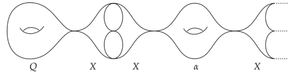
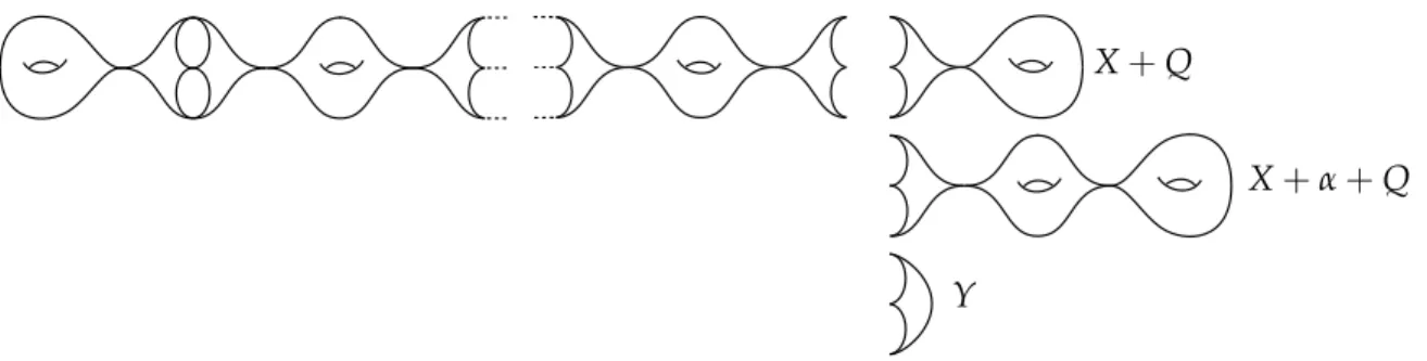
Now we argue similarly for each subsequent sequence of three pairs of pants. After pinching these lift to X, α and X. (The α appears because via Riemann-Hurwitz and the monodromy, the second pair of pants lifts to a two holed torus with an automorphism of order 3 and two fixed points. In light of lemma3.7, by pinching the subsurface is α.) As such the lift of our surface is
where we somewhat loosely denote by + a type of “stable” sum of surfaces as in the following figure.
Q X X α X
Figure 5: The beginning of the lift
There are three cases to consider, depending uniquely on properties of the number g (or equivalently r).
Case 1: r ≡0 mod 3
In this case, after obtaining in the lift Q+X we have lifted T−2 copies of X+α+X. There
is now a final triple of branch points with the same monodromy and the curve γ11surrounds two of the branch points to form a pair of pants. As in the initial lift, this pair of pants lifts to Q. The surface then ends with X+Q. The final surface is (in our loose notation)
Q+X+
∑
T−2
(X+α+X) +X+Q.
Case 2: r ≡1 mod 3
Arguing similarly we obtain in this case Q+X+
∑
T−1
(X+α+X) +X+α+Q.
Case 3: r ≡2 mod 3
Arguing similarly we obtain in this case Q+X+
∑
T−1
(X+α+X) +Y
where by Y we mean the unique hyperbolic thrice punctured sphere. These cases are illustrated in figure6.
4. ONE DIMENSIONAL CYCLIC p-GONAL LOCI FOR PRIME p
>
3In light of the above, the incurable optimist might believe that the set of cyclic p-gonal surfaces for p prime is always connected in the completion of moduli space. In this section
X+Q
X+α+Q
Y
Figure 6: The full surface with the three possible end cases we show that this fails in general.
Recall that f : S→C is a cyclic p-gonal covering if it is regular cyclic covering. We recallˆ
the well-known characterization of such coverings in terms of monodromy.
Proposition 4.1. The covering f →C is a cyclic p-gonal covering if and only if there is a canonicalˆ
set of generators{x1, . . . , xr}with monodromy representation as follows:
ωf : π1(Cˆ \ {b1, . . . , br}, o) → Σp
xi 7→ (1, 2, . . . , p)ji, ji ∈ {1, 2, . . . , p−1}.
In this case note that we have
r = 2g
p−1 +2. As the product of the generators is the identity we have:
r
∑
i=1ji ≡0 mod p.
We now pass to a first example that will serve as a guide for what follows. 4.1. Cyclic5-gonal surfaces in genus 4
Let g=4. Following Nielsen, there are three topological types of cyclic 5-gonal coverings of genus 4 surfaces. There are given by the monodromy types
ωf : π1(Cˆ \ {b1, . . . , b4}, o) →<t >⊂Σ5
with t := (1, 2, 3, 4, 5)and with the property that the order of ωf(xi)is 5. These are given by
2. ωf(x1) =ωf(x2) =t and ωf(x3) =ωf(x4) =t4,
3. ωf(x1) =t, ωf(x2) =t2, ωf(x3) =t3and ωf(x4) =t4.
Note that this means that there are three topological types of cyclic 5-gonal surfaces, each given by the monodromies specified above. It is a well known fact that they live in distinct connected components of the (cyclic) 5-gonal locus inM4(see [CI1]). Specifically i=1, 2, 3 each
Mi4 := {S∈ M4 | there exists a cyclic 5-gonal morphism f : S→C of type iˆ }
is connected with dimCMi
4 =1 and that for i, j=1, 2, 3
Mi
4∩ M
j 4 =∅
if i6=j.
Our observation in this setup is the following: Theorem 4.2.
M14∩ M4j =∅
for j6=1 and
M24∩ M34 6=∅
Proof. In this proof, we assume that our surfaces are endowed with their unique hyper-bolic metrics. In particular the cyclic 5-gonal covering becomes an automorphism of the hyperbolic metrics.
Assume that S ∈ M4j \ M4. Then there exists for k = 1, j sequences{Si(k) ∈ M4} → S. Denote µ(ik) ⊂Sithe multicurve whose length approaches 0 as i→∞.
If we denote a(ik)the cyclic 5-gonal automorphism of S(ik), the multicurves µ(ik)must be a(ik)-invariant. In particular, it is important to observe that µ(ik)is the lift of a simple closed geodesic on Si(k)/< a(ik) >. This follows from the fact that µi(k)descends on Si(k)/< a(ik)>
to a connected curve whose length must also go to 0 and by Lemma2.1, this curve cannot pass through the fixed points of order 5.
There are three different topological types of simple closed geodesics on an orbifold of genus 0 with 4 points of order 5 (the quotients S(ik)/< a(ik) >are all of this type). Observe that there is a unique genus 0 hyperbolic orbifold with one cusp and two orbifold points of order 5. As such, there are at most three possible stable surfaces (up to isometry) in each
Each simple closed geodesic on a S(ik)/<a(ik)>surrounds two orbifold points on one side and two on the other. Once we pinch, we obtain pants with two orbifold points and a cusp. We are interested in the isometry types of surfaces that these pants lift to. Their isometry types are clearly determined by the monodromies but also clearly different monodromies can lift to isometric pieces. For instance, if the two monodromies are t, t or t−1, t−1, then the pants lift to isometric pieces. We claim that the pants can lift to exactly three isometrically distinct surfaces:
Case 1:{t, t},{t−1, t−1}
In this case we get a genus 2 surface with one cusp with an automorphism of order 5 with two fixed points with the same rotation index. Forgetting the cusp, this is a conformally the unique genus 2 surface with a conformal automorphism of order 5. We denote this surface by P1.
Case 2:{t, t2},{t, t3},{t2, t4},{t3, t4}
In this case we get a genus 2 surface with one cusp with an automorphism of order 5 with two fixed points but with the different rotation indices. Note that although this surface is conformally equivalent to the one in the previous case when one forgets the cusp, they are not isometric as the topological types of the coverings are different, and a result by [G] tells us that there is only one topological type of cyclic coverings from a given surface of genus 2 to the sphere. We denote this surface by P2.
Case 3:{t, t−1} = {t, t4},{t2, t3}
In this case, we obtain a sphere with 5 cusps with an automorphism of order 5 with two fixed points and which permutes the cusps. We denote this surface by P3.
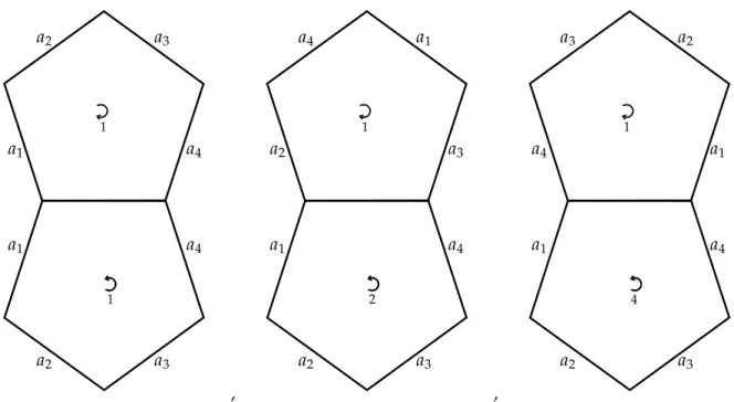
Let us pause for a moment to consider the geometries of P1, P2 and P3. They can be
constructed as follows. Consider the unique regular hyperbolic ideal pentagon. (In figures
7we have schematically drawn this pentagon as Euclidean.) Now paste two copies along a common edge “without” shearing, i.e, such that the geodesic between the two centers of the pentagons meets the common edge at a right angle. This gives an octogon. All three surfaces can now be obtained by pasting the octogon in different ways as illustrated in the figures. The fact that these are indeed the correct surfaces follows from the fact that they have the appropriate isometry groups which descend to the pants with the appropriate monodromies and by the uniqueness arguments outlined above.
We now look at which surfaces can lie on the boundary of the different strata. For M1
, , a1 a1 a2 a2 a3 a3 a4 a4 1 1 a1 a2 a2 a4 a3 a1 a4 a3 2 1 a1 a4 a2 a3 a3 a2 a4 a1 4 1
Figure 7: The surfaces P3(sphere), P1(torus), P2(genus 2)
surround two orbifold points whose monodromy is t. The other pair of pants has points with monodromy{t, t2}. Thus the surface is given by a copy of P1and a copy of P2which
are glued at their cusps. We denote the surface thus obtained somewhat loosely by P1+P2.
ForM2
4 there are two distinct possibilities, i.e., the monodromies are given by the pairs
{t, t},{t−1, t−1}or{t, t−1},{t, t−1}. In the first case we obtain P
1+P1 and in the other
P3+P3.
ForM3
4we obtain also only two distinct possibilities, i.e., the monodromies are given by
the pairs{t, t2},{t3, t4}or{t, t3},{t2, t4}. This gives P
2+P2and P3+P3.
By the above analysis it is clear thatM2
4andM34meet at the boundary (at a unique point
P3+P3) andM14is disjoint from the other two.
4.2. p-gonal with p prime and g= p−1
We now consider a generalization of the above example. The proof follows the same outline is indeed almost identical.
Let g= p−1. Again following Nielsen, we can classify topological types of cyclic p-gonal coverings of genus p−1 surfaces. There are given by the monodromy types
with t := (1, 2, . . . , p)and with the property that the order of ωf(xi)is p. For simplicity, we
have indexed the ωf by their type. These are given by
1. ω1(x1) =ω1(x2) =ω1(x3) =t and ω1(x4) =tp−3,
2. ω2(x1) =ω2(x2) =t, and ω2(x3) =ω2(x4) =tp−1,
3. ω3,i(x1) =t, ω3,i(x2) =ti, ω3,i(x3) =t−iand ω3,i(x4) =tp−1,
4. ω4,i(x1) =t, ω4,i(x2) =t, ω4,i(x3) =tiand ω3,i(x4) =tp−2−i,
5. ω5,i,j(x1) =t, ω5,i,j(x2) =ti, ω5,i,j(x3) =tjand ω5,i,j(x4) =tp−1−i−j.
Note that types 3, 4, and 5 contain several subtypes of monodromies. As before we consider the strata of moduli space corresponding to each type. Specifically we denote
MpI−1 :=S∈ Mp−1 | there exists a p-gonal morphism f : S→C of type Iˆ }
We can now state our main theorem.
Theorem 4.3. Mp(5,i,j−1)is completely isolated inBg.
Observe that for the theorem to be true,Mp(5,i,j−1)must be completely isolated inBgand this
is true as was shown in [CI2].
Proof. Our first observation is that up to isometry, there are exactly p+21 hyperbolic surfaces with an automorphism of order p with two fixed points and whose quotient is a sphere with a single cusp. To see this, we will generalize the case by case analysis of the lifts of the pairs of pants in the proof of Theorem4.2.
Consider Op,p,∞be the (hyperbolic) orbifold of genus 0 with two orbifold points of order p and a cusp. The cyclic p-gonal coverings are given by the monodromies
θ : π1Orb(Op,p,∞) =<y1, y2|y1p =y p
2 >→<t >⊂Σp
(where π1Orb denotes the orbifold fundamental group) and we define a map
(y1, y2) 7→ (θ(y1), θ(y2)) = (ta, tb).
By the result of Gonzalez-Diez [G] , two such maps(ta, tb)and(ta0, tb0)induce equivalent
surfaces if and only if there exists a c such that
and
b0 ≡cb mod (p)or b0 ≡cb−1 mod (p).
We denote the monodromy types by(i, j)if it is represented by(ti, tj). Observe that in each equivalence class, there is a representative of type(1, j).
We denote Pj the covering of Op,p,∞given by the monodromy of type(1, j).
We proceed as in the example and we now analyze the surfaces obtained at the limit in the different types discussed in the beginning of the section.
Type 1: Here we obtain P1+Pp−3as we have the lift of a Op,p,∞of type(1, 1)and one of
type(1, p−3). We proceed in the same way for each of the subsequent types. Type 2: P1+P1, Pp−1+Pp−1 Type 3: Pp−1+Pp−1, Pi+Pi, P−i+P−i where 2≤ i≤ p−21 Type 4: P1+Pp−i−2 i , Pi +Pp−i−2 where 2≤ i≤ p−21 Type 5: Pi+P−1−i+1 j , Pj+P−1−j +1 i , Pj i +Pp−1−i−j where 2≤ i≤ p−21, i<j≤ p−3 with p−1−i−j6∈ {1, i, j, p−1,−i,−j}
Through the equivalences above, it is straightforward to check that the surfaces appearing in Type 5 do not appear in any of the other cases. It remains to show that they are distinct from each other.
Let us show that the surfaces of type 5 are distinct for distinct equisymmetric sets inMp−1.
We must prove that if either: 1. Pi+P−1−i+1 j =P 0 i +P−1−i0 +1 j0 , 2. Pi+P−1−i+1 j =Pj 0 i0 +Pp−1−i0−j0or 3. Pj i +Pp−1−i−j = Pj i +Pp−1−i−j
thenMp(5,i,j−1) = Mp(5,i−10,j0).
Let us assume that we are in the situation described in the point 1 (the other cases are similar). If i=i0and−1−i+j1 = −1−i0+j01then it is clear that(i, j) = (i0, j0). If i= −1−i
0+1 j0
and i0 = −1− i+1
j then using automorphisms of π1(Cˆ \ {b1, b2, b3, b4}, o) and Cp and
This proves that the setsMp(5,i,j−1)are isolated among the set of cyclic p-gonals. We now show that they cannot meet another type of surface from the branch locus on the boundary. Suppose the contrary. The limit surface S will have then h the p-gonal automorphism and an automorphism of different type, i.e., non p-gonal. This second automorphism h0will induce an automorphism on the quotient S/h because h is normal inside the automorphism group of the surface by [G] . Now h0 descends to an autormorphism ¯a : Op,p,∞such that
¯a∗ : π1Orb(Op,p,∞) →π1Orb(Op,p,∞)
has the property ¯a∗◦θ =θ(where θ is the monodromy of the piece Op,p,∞).
However the monodromies θ for the Piappearing in the boundary of strata of type 5 do not
allow such properties.
We remark that this theorem provides a number of one dimensional completely isolated strata. Via a straightforward calculation this number can be shown to be quadratic in p but note that they are not necessarily distinct inMgas several could correspond to the same strata.
REFERENCES
[AP] Achter J. D.; Pries R., The integral monodromy of hyperelliptic and trielliptic curves. Math. Ann. 338 (2007) 187-206.
[BCIP] Bartolini G.; Costa A. F.; Izquierdo M., Porto, A. M., On the connectedness of the branch locus of the moduli space of Riemann surfaces. Rev. R. Acad. Cienc. Exactas F´ıs. Nat. Ser. A Math. RACSAM 104 (2010), no. 1, 81-86.
[BCI1] Bartolini, Gabriel, Antonio F. Costa, and Milagros Izquierdo: On the connectivity of branch loci of moduli spaces, Annales Academiae Scientiarum Fennicae, 38 (2013), no. 1, 245-258.
[BCI2] Bartolini, Gabriel; Costa, Antonio F.; Izquierdo, Milagros On isolated strata of p-gonal Riemann surfaces in the branch locus of moduli spaces. Albanian J. Math. 6 (2012), no. 1, 11-19.
[BCI3] Bartolini, Gabriel; Costa, Antonio F.; Izquierdo, Milagros On isolated strata of pentagonal Riemann surfaces in the branch locus of moduli spaces. Computational algebraic and analytic geometry, 19-24, Contemp. Math., 572, Amer. Math. Soc., Provi-dence, RI, 2012.
[BI] Bartolini, Gabriel; Izquierdo, Milagros On the connectedness of the branch locus of the moduli space of Riemann surfaces of low genus. Proc. Amer. Math. Soc. 140 (2012), no. 1, 35-45.
[B] Broughton, S. Allen. The equisymmetric stratification of the moduli space and the Krull dimension of the mapping class group. Topology and its Applications, 37 (1990) 101-113.
[BSS] Buser, Peter; Sepp¨al¨a, Mika; Silhol, Robert. Triangulations and moduli spaces of Riemann surfaces with group actions. Manuscripta Math. 88 (1995), no. 2, 209-224. [CI1] Costa, Antonio F.; Izquierdo, Milagros Equisymmetric strata of the singular locus
of the moduli space of Riemann surfaces of genus 4. Geometry of Riemann surfaces, 120-138, London Math. Soc. Lecture Note Ser., 368, Cambridge Univ. Press, Cambridge, 2010.
[CI2] Costa, Antonio F.; Izquierdo, Milagros. On the existence of connected components of dimension one in the branch locus of moduli spaces of Riemann surfaces, Math. Scand., 111 (2012), no. 1, 53-64
[CI3] Costa, Antonio F.; Izquierdo, Milagros. On the connectedness of the branch locus of the moduli space of Riemann surfaces of genus 4. Glasg. Math. J. 52 (2010), no. 2, 401-408.
[DP] Dryden, Emily E.; Parlier, Hugo. Collars and partitions of hyperbolic cone-surfaces. Geom. Dedicata, 127 (2007) 139-149.
[G] Gonz´alez-D´ıez, Gabino. On prime Galois covering of the Riemann sphere. Ann. Mat. Pure Appl. 168 (1995) 1-15
[K] Kulkarni, Ravi S. Isolated points in the branch locus of the moduli space of compact Riemann surfaces. Ann. Acad. Sci. Fenn. Ser. A I Math. 16 (1991), no. 1, 71-81.
[MS] Macbeath, A. M.; Singerman, D. Spaces of subgroups and Teichmller space. Proc. London Math. Soc. (3) 31 (1975), no. 2, 211256.
[Na] Natanzon, S. M. Moduli of Riemann surfaces, real algebraic curves, and their su-peranalogs. Translations of Mathematical Monographs, 225. American Mathematical Society, Providence, RI, 2004. viii+160 pp. ISBN: 0-8218-3594-7.
[Ni] J. Nielsen, Die Struktur periodischer Transformationen von Flchen, Math.-fys. Medd. Denske Vid. Selsk. 15 (1937), 1-77.
[ST] Seifert, Herbert; Threlfall, Willian. A Textbook of Topology. Academic Press, Orlando, 1980.
[Se] Sepp¨al¨a, Mika. Real algebraic curves in the moduli space of complex curves. Composi-tio Math. 74 (1990), no. 3, 259–283.
[SeSo] Sepp¨al¨a, Mika.; Sorvali, Tomas. Affine coordinates for Teichm ¨uller spaces. Math. Ann. 284 (1989), 165-176.
Addresses:
Antonio F. Costa, Departamento de Matematicas Fundamentales, Facultad de Ciencias, Senda del rey, 9, UNED, Madrid, Spain
Milagros Izquierdo, Department of Mathematics, University of Linkoping, Sweden Hugo Parlier, Department of Mathematics, University of Fribourg, Switzerland Email:[email protected] [email protected] [email protected]